Market fundamentals, competition and natural-gas prices
Daan Hulshof
a, Jan-Pieter van der Maat
a, Machiel Mulder
a,b,na
Faculty of Economics and Business, University of Groningen, The Netherlands b
Authority for Consumers & Markets, The Netherlands
H I G H L I G H T S
We analyse the development of the day-ahead spot price at TTF over 2011–2014. The oil price had a small impact on the gas price, while the coal price had no effect. Changes in the concentration on the supply side did not affect the gas prices. The gas prices are predominantly determined by weather and storage availability. Policies to integrate gas markets foster gas-to-gas competition.
a r t i c l e i n f o
Article history:Received 15 July 2015 Received in revised form 12 December 2015 Accepted 14 December 2015 Available online 7 January 2016 Keywords:
Natural gas prices Gas hubs Competition Time series analysis
a b s t r a c t
After the liberalisation of the gas industry, trading hubs have emerged in Europe. Although these hubs appear to be liquid market places fostering gas-to-gas competition, the efficiency of the gas market remains a topic of interest as a fair share of gas is still traded through long-term contracts with prices linked to the oil price while the number of gas suppliers to the European market is limited. In order to assess the efficiency of the gas market, we analyse the day-ahead spot price at the Dutch gas hub over the period 2011–2014. Wefind that the oil price had a small positive impact on the gas price. Changes in the concentration on the supply side did not affect the movement in gas prices. The availability of gas in storages and the outside temperature negatively influenced the gas price. We alsofind that the gas price was related to the production of wind electricity. Overall, we conclude that the day-ahead gas prices are predominantly determined by gas-market fundamentals. Policies to further integrate gas markets within Europe may extend this gas-to-gas competition to a larger region.
&2015 The Authors. Published by Elsevier Ltd. This is an open access article under the CC BY license (http://creativecommons.org/licenses/by/4.0/).
1. Introduction
The institutions of the European gas market have changed considerably in the last decade. Trading at gas hubs such as the National Balancing Point (NBP) in the United Kingdom and the Title Transfer Facility (TTF) in The Netherlands have gained rapid importance (Heather, 2012). Parallel to this development, the convention of explicitly linking the gas price to the oil price has lost importance. Because oil and gas were substitutes in many processes, oil indexation became the leading pricing mechanism for gas in the 20th and early 21st century in Europe. Since the gas market has changed significantly in recent years, however, gas-to-gas competition seems to have become the dominant price me-chanism (IGU, 2014). Moreover, recent evidence shows that
national gas markets in North-west Europe are increasingly in-tegrated with each other, resulting in a North-west European market covering countries as the UK, France, The Netherlands, Belgium, Germany, Denmark, Italy and Austria (Growitsch et al., 2012; Kuper and Mulder, 2014; Neumann and Cullmann, 2012; Petrovich, 2013;Timera Energy, 2013).
Nevertheless, there are still concerns regarding the intensity of competition within the European gas market as the dispersion of reserves is concentrated while the number of suppliers is limited. Iffirms are able to exert market power, above-competitive gas prices may result which reduces consumer welfare. Furthermore, the gas market faces periodical shocks in both supply and demand, which distort the gas prices. For example, the extremely cold weather throughout Europe in February 2012 led to a (perceived) tightness of the market supply. In addition, the Fukushima disaster and the consequent nuclear shutdown in Japan led to a substantial increase in Asian demand for LNG.
A number of different approaches to understand the factors behind gas prices have been used in the recent literature. Several Contents lists available atScienceDirect
journal homepage:www.elsevier.com/locate/enpol
Energy Policy
http://dx.doi.org/10.1016/j.enpol.2015.12.016
0301-4215/&2015 The Authors. Published by Elsevier Ltd. This is an open access article under the CC BY license (http://creativecommons.org/licenses/by/4.0/). nCorresponding author at: Faculty of Economics and Business, University of
Groningen, The Netherlands.
authors have established long run co-integrating relationships between gas and oil prices (e.g.Asche et al., 2006;Regnard and Zakoïan, 2011, for the European gas market andErdős, 2012;Villar and Joutz, 2006, for the US gas market). Some papers have em-phasised the role of other supply and demand fundamentals, in particular for the short-run price development because energy commodities differ in fuel density and accordingly in production, transportation and environmental cost (Smith, 2004; Mu, 2007; Brown and Yücel, 2008).Ramberg and Parsons (2012)show that the vector error-correction models typically applied in the co-in-tegration framework do not perform very well in explaining short run gas price development. In another fashion,Nick and Thoenes (2014) investigated the effect of market shocks in a structural vector autoregressive (SVAR) model and found that temperature, storage and supply shocks lead to relatively short lasting effects on the gas price whereas oil and coal price shocks result in more persistent effects on the gas price.
With the strongly reduced share of explicit oil indexation and the reduced options for short run gas–oil substitution in North-west Europe (Stern, 2007,2009), the supply and demand funda-mentals might have become more important for the development of the gas price at liberalised hubs. This is the reason that we es-timate a reduced form model of the gas price which enables us to assess the impact of the key fundamental factors on the short term movements of the gas price.
The main question addressed in this paper is: what drives natural gas prices at liberalised European gas markets? More specific, to what extent is the gas price tied to oil and/or coal and what is the effect of other supply and demand fundamentals? This paper contributes to the literature by providing a comprehensive empirical analysis, facilitated by the collection of data for a broad set of gas-market variables. Moreover, while other papers have largely focussed on a single national market, we include a number of variables related to the North-west European market for natural gas. We define the North-west European gas market as the mar-kets in Austria, Belgium, Denmark, France, Germany, Italy, the Netherlands and the UK. The gas networks in these countries are closely connected. In addition, gas is being exported from the Netherlands to each of these markets, which fosters the integra-tion of the markets. As a result, changes in fundamental factors affecting supply or demand in these countries may also affect the gas price at the TTF.
This paper analyses the development of spot market gas prices at the TTF hub over the period 2011–2014 by assessing the con-tribution of a number of supply and demand fundamentals. We focus at the TTF since it is viewed as a suitable reference hub which is the most liquid and mature trading hub in continental Europe (Heather, 2012). The annual volume delivered at TTF is about 40 bcm while the total gas consumption in the Netherlands is about 45 bcm, which indicates that the TTF is important for the Dutch gas market (GTS, 2012). Moreover, the TTF appears to be strongly integrated with gas hubs in neighbouring markets such as the NCG in Germany (ACM, 2014;Kuper and Mulder, 2014). As a result, the prices on TTF and the other hubs show almost the identical pattern. The day-ahead price is appropriate because it refers to one of the most liquid traded products, which makes that the price of this product is strongly related to the underlying factors (Heather, 2010). The liquidity of the day-ahead products follows from the depth of this market, which is significantly higher than for the other products (ACM, 2014).1Hence, in the short run, fundamental supply and demand factors are especially important for the development of the day-ahead price. The fundamentals
include the outside temperature, the macroeconomic develop-ment, the price of substitute fuels, the concentration in physical terms on the supply side to the European market, the expected level in global gas reserves and the development in renewable energy. While assessing the impact of these factors, we control for a number of incidental events such as the inability of Gazprom to meet unexpected demand and the Fukushima disaster.
Wefind no evidence of a strong tie between the spot prices of natural gas, crude oil and coal over 2011–2014. The development of the gas price is mainly determined by own fundamentals. Though, a short-run link between the three energy commodities is present via arbitraging between oil indexed gas and hub gas as well as via fuel competition in the power market. Despite being a fairly concentrated market, the changes in the daily gas price do not depend on the changes in the structure on the supply side. Overall, we conclude that the day-ahead gas prices are pre-dominantly determined by gas-market fundamentals.
The remaining of this paper is organised as follows.Section 2 describes the method of research which includes a description of the variables which are used to measure the fundamentals behind the gas price. This section also presents the data which is used to estimate the model.Section 3presents and discusses the results. The conclusions and policy recommendations are given inSection 4.
2. Method and data
We estimate a reduced-form model of the gas price. This model is based on the idea that the gas price is a function of shifts in the demand and the supply curves. To determine the effect of supply and demand factors on the gas price the equation PTTF= (ϕX Y, )is estimated, where Xand Y contain the demand and supply vari-ables and PTTFreflects equilibrium gas prices on both the supply
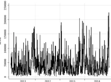
and demand schedules, i.e. the points of intersection of both curves. In this section we elaborate on the key factors affecting the demand and supply curves behind the TTF price. The dataset for the quantitative analysis comprises data from 4/1/2011–30/12/ 2014. It consists of daily observations except for the macro-economic indicator which is available on a monthly frequency. The dataset does not include prices for weekends limiting the analysis to weekdays only.Table 1gives an overview of all variables, how they are measured and the data sources. SeeFig. 1for the day-ahead gas price
2.1. Price of oil
A factor which may affect both the demand and the supply of gas is the price of oil. The price of oil is relevant because of sub-stitution properties of gas and oil (Villar and Joutz, 2006). Sub-stitution is primarily relevant in the electricity generation and the heavy industry. If the price of oil rises, burning gas becomes re-latively cheaper, increasing the demand for gas which results in an upward pressure on the gas price. However, Stern (2007,2009) argues that short-run fuel switching is hardly relevant anymore in West Europe because oil has virtually disappeared in most sta-tionary energy sectors, maintenance of dual-fuel burners is ex-pensive, tight environmental standards as well as the inefficiency of using oil in new gas burning technologies.
In addition to the apparent lack of short-run substitutability there are several other reasons why oil and gas should have dis-tinct price dynamics (Smith, 2004). The transportation costs differ and there are differences in the costs of production, processing, storage and environment. Moreover, the differences in character-istics have led gas and oil prices to be determined in different geographical market places, as noted by Ramberg and Parsons 1
The depth of a market is measured by the number of additional lots of 30 MW traders could sell or buy without influencing the price (ACM, 2014).
(2012). Although regional differences between types of crude oil exist, such as Brent and West Texas Intermediate, their prices are usually correlated. Natural-gas prices at the hubs, however, are much more subject to regional supply and demand conditions. The regional gas markets are not independent from each other, and perhaps are becoming increasingly tied (Stern and Rogers, 2014), but regional prices can move in very different directions as can be seen from the recent divergence in European and North-American gas prices (Mulder, 2013).
Even if the supply and demand dynamics of gas and oil differ and there is a lack of short run substitution, the price of oil
in-fluences the price of gas if the gas price is explicitly linked to the oil price in contracts, as was a common practice in Europe since the 1960s. The key question is how important this price me-chanism still is for the West European market. The answer is somewhat difficult to obtain because most information sits in the private domain. The IGU (2014) nevertheless estimates that the share of oil indexation in North-west Europe decreased from 72% in 2005 to 20% in 2013.
Because of the remaining oil-indexation contracts, traders try to arbitrage between spot and contract gas insofar this is possible given the minimum take obligations in these contracts (Stern and
Rogers, 2014). If the gas spot price is below the oil-indexed con-tract price, the demand at hubs for spot priced gas will increase whereas demand for oil indexed gas decreases. This will increase the price of spot gas. Consequently, buyers with long term con-tracts try to decrease their nominations up to the minimum take obligation resulting in lower upstream production and total mar-ket supply. The opposite mechanism holds if the gas spot price is above the oil-indexed contract price.
Because of these remaining arbitrage possibilities, we include the price of oil as an independent variable. The spot price of Brent oil is the most relevant crude oil price for the West European market. Prices are specified in US Dollar per barrel. In order to account for exchange ratefluctuations the US Dollar per barrel, the price is divided by the day-ahead US Dollar/Euro exchange rate to obtain a day-ahead Euro per barrel price.
The other relevant variables for inter-fuel competition that are included are the price of North-west European coal and the price of CO2 in the European Union Emissions Trading Scheme, both in Euro per tonne as reported by Bloomberg (Fig. 2).
2.2. Market structure
Although a large numbers of traders are active on the gas hubs like TTF, the supply to the gas market is concentrated because of the limited number of producers. The main sources of supply to the North-west European market are‘indigenous’ production in The Netherlands and UK as well as imports from Russia, Norway, Algeria and LNG, primarily coming from Qatar. This supply can be distinguished in inflexible and flexible supply (Timera Energy, 2013). Inflexible supply of gas include pipeline-contract gas up until take-or-pay volumes, destination-inflexible LNG cargoes (mainly into Southern Europe) and indigenous production which do not seem to respond to hub price signals in practice. While these tranches may have some flexibility (e.g. to allow for sea-sonality), they generallyflow irrespective of the absolute level of hub prices and have therefore no primary impact. The flexible supply of gas consists of pipeline-contract gas between the take-or-pay and maximum annual contracted volume, un-contracted pipeline import flexibility from mainly Norway and Russia and
flexible LNG supply.
The limited number of producers of gas to the European market raises some concerns on the degree of competitiveness of the gas Table 1
Variable definitions.
Description Source Frequency (unit)
Heating degree days West European gas consumption weighted average number of heating degree days
European Climate Assessment and Dataset (ECA&D) Daily (degree celcius) TTF gas price Title Transfer Facility day-ahead natural gas price ICIS Heren Daily (€/MWh) Brent oil price European Brent crude oil spot price ICIS Heren Daily (€/Barrel) NW European coal price Northwest European coal price Bloomberg Daily (€/Tonne) CO2 price Price of European carbon credits Bloomberg Daily (€/Tonne) Gas storage Deviation in the dailyfilling degree of West European gas
storage facilities from the daily averagefilling degree of the past 3 years
Gas Infrastructure Europe (GIE), Cedigaz Underground Gas Storage Database (CUGS) and Gasunie Transport Services (GTS)
Daily (Percentage points) Herfindahl-Hirschman
in-dex (HHI)
Aggregated squared market shares of suppliers Eclipse-Own calculations Daily (index [0,10000]) Macroeconomic indicator Monthly gas consumption weighted average production
volume index of the manufacturing sector in West Europe
Eurostat Monthly (indice)
Wind electricity Germany Day-ahead prediction of electricity generation from Ger-man wind power
50 Hertz, Amperion, TenneT, TransnetBW Daily (MWh) Global discoveries Dummy indicating announcement and period after large
global gas discoveries
WoodMackenzie –
Fukushima nuclear disaster Dummy separating the period before and after the Fu-kushima nuclear disaster on the 11thof March 2011
– –
Cold spell in Europe 2012 Dummy indicating the period of extremely cold weather throughout Europe in February 2012
– –
Fig. 1.TTF gas price and Brent crude oil price per week day, 2011–2014 (Source: ICIS Heren).
market. Typically, the production and export in one country is dominated by large state-controlled companies. This gives rise to concerns regarding oligopolistic market behaviour and profound effects following supply disruptions. Iffirms hold a strategic po-sition, they are able to execute market power resulting in prices above the competitive level. It should be noted that other parts of the gas market than production affect the degree of competition as well. Gas producers are often not responsible for transportation and each part of the value chain has its own dynamics. However, production is essential to understand competition in the market for gas as it are producers who determine the gas volumes the other value chains work with (Brakman et al., 2009).
In terms of industry structure the gas market is commonly described by a Cournot configuration as the market trades in the homogenous good gas,2prices observed are above marginal costs, quantity is the strategic variable and a limited number offirms supply the market. To assert the degree of competition in a market the Herfindahl-Hirschman index (HHI) is widely used. The HHI is an indicator for market concentration, defined as: HHI= ∑in=1Si
2 whereSiis the market share offirmiandnthe number offirms;
i.e. the aggregate of the supplier's squared market shares. As such it is an indicator for the structure of a market and signals the potential for the exertion of market power byfirms. We, therefore, include the HHI in our model which is based on the supply coming from different players to the North-west European market.
The supply data includes supply from Russia, Norway, Algeria, LNG, The Netherlands and UK.3 The daily supply is based on the supply entering the system via pipelines from Norway, The Neth-erlands, UK, Russia and Algeria and total LNG supply (Fig. 3and Table 2).4The data does not allow us to determine the source of LNG entering the system and therefore LNG is treated as a single market supplier.
Daily production data for The Netherlands and UK is readily available, but the relevant export of other suppliers to North-west Europe is not. To determine imports via the pipeline system from the most important‘foreign’suppliers, Russia, Norway and Algeria, all those gas transmission points at the‘border’of the market via
which production of the respective suppliers can enter the pipe-line system in Central and West Europe are identified.5Generally, there exists more than one receiving Transmission System Op-erator (TSO) at a gas transmission border point. The physicalflow in MWh reported by each TSO at border points is extracted from Eclipse. For Norway 16 relevant border points are identified, ar-riving in The UK, France, Belgium, The Netherlands and Germany (see appendix A for a list of all the identified entry points for each non-indigenous supply source). For Russia, 4 relevant border points in 3 countries are identified: one for gas entering via Uk-raine and Slovenia, two for the direct connection between Ger-many and Russia via the Nordstream pipeline and one for gas Fig. 2.Coal price and CO2 price, per day, 2011–2014 (Source: Bloomberg). (a) Northwest European Coal price (b)European CO2 price.
Fig. 3. Daily average market share per country per year, 2011–2014 (source: own calculations based on data from Eclipse).
Table 2
Daily average gas supply per country/source (GWh).Source: Eclipse.
2011 2012 2013 2014 LNG 2367 1674 1183 1055 Russia 2821 2675 3257 2829 Norway 2643 3095 3045 3019 The Netherlands 2098 2151 2261 1875 UK 1181 1032 981 1001 Algeria 994 1164 970 909 Total 12,104 11,791 11,697 10,688
2Quality differences in terms of energetic content exist, however, trade and prices are based on energy content rather than physical volume.
3
It should be noted that because production in other European countries (e.g. Germany, Denmark and Italy) is excluded, total supply is somewhat under-estimated and the market shares and HHI are somewhat overunder-estimated. The joint production in the omitted countries is, however, small.
4
It is not possible to distinguish the type of supply byflexibility. The vast majority of the production from Norway, Algeria and Russia enters the European system via pipelines, however, these countries also ship some LNG to North-west Europe.
5
Gas from Russia to North-west Europe is measured at the border points Polen–Belarus and Slowakije–Ukraine.
entering Europe via Belarus and Poland. Algerian production en-ters the pipeline system at 4 border points in Spain and Italy. Regarding LNG, 18 relevant terminals in 7 countries are identified. The production data limits us to study the period after 1/1/2011 as data is largely unavailable prior to this date.
The total market supply is estimated as the aggregate of supply from each source and consequently the HHI is constructed by summing over all the squared market shares of the 6 supply sources. The HHI has increased from approximately 1900–2100 from 2011–2014 (seeFig. 4).6 Table 2shows that LNG supply to Europe has more than halved in that period, which is an important contribution to the increase in the HHI. The decrease in European LNG supply occurs simultaneously with the surge in Asian LNG demand after 2011. The increases in supply of the two largest suppliers, Russia and Norway, have contributed to the increase in the HHI (Fig. 3).
2.3. Storage
Storage of gas plays an important role for hub prices as storages can be used for inter-temporal arbitrage. The theory of gas storage states that the level of inventories affects the difference between spot and futures gas prices (Kaldor, 1939; Brennan, 1958; Fama and French, 1987).Brown and Yücel (2008)find that natural gas storage has an effect on the price of gas. Due to the fact that the consumption of gas is seasonal while the production has generally more limita-tions to adapt its levels accordingly, storages can be used.7 These inventories arefilled in the summer for use in the winter. In addition, above normal heating and cooling-degree days put upward pressure on the gas price. Inventories above the seasonal norm depress prices while inventories below the seasonal norm have a positive effect on prices. Disruptions in production might also have a positive effect on prices. The above authors calculate a storage differential as the dif-ference between storage in a given week and the average for that week over the past five years. These authors find that when the
filling degree of a natural gas storage facility is above the seasonal norm, it depresses natural gas prices.
Traditionally, storage capacity in Europe is mainly used to smooth out the seasonal demand shape. The storage facilities
demand gas in the warm period of the year when gas is injected and they become suppliers in the colder periods as gas is with-drawn. Technical restrictions on injection and withdrawal result in some inflexibility of storage facilities to respond to price signals in the short term. However, many storages currently under con-struction are being built for short-run arbitrage opportunities between spot and contract gas (Stern and Rogers, 2014). Con-sidering that most storage facilities largely operate on a yearly planned cycle,Cartea and Williams (2008)argue that deviations from the expected storage cycle are most relevant for spot price development. If inventory levels are lower than expected, storage operators demand a higher price and vice versa for storage levels above expectations.
Following the approach taken byCartea and Williams (2008) andBrown and Yücel (2008), we calculate a storage differential. This storage differential is calculated as the difference between the storage on a given day and the average for that day over the pastn
years. This can be represented as follows:
(
)
∅ = − * +… + * * ( ) − − S n S n S 1 1 1 t t t 365 t n 365where St is the weighted percentage of total capacityfilled on a
given day and ∅tis the actual deviation from the averagefilling
grade of the pastnyears, measured in percentages. In their paper, Brown and Yücel use a period ofn=5years for their analysis. In this paper, we will use a period of 3 years as reliable data con-cerning thefilling grade of storages in the respective countries is available as from the end of 2007.
In order to capture the impact of storage, a variable is con-structed which measures the deviation in the utilisation level (i.e.
filling degree) from the average North-west European storage utilisation level. The countries that possibly influence the TTF price through their storage facilities are: Austria, Denmark, France, The United Kingdom, Germany, The Netherlands, Belgium, and Italy.8 Data for the storage variable are available on a weekly basis from October 2007 onwards. From the 1st of January 2010, data are available on a daily basis.
Fig. 5 clearly shows two peaks in the beginning of the time period of analysis. Thefirst two peaks are the winters of 2011 and 2012 respectively, which were relatively mild, while the winter of 2013 was colder than average. The winter of 2014 was a very mild winter, even more than the winters of 2011 and 2012. Storages were 13% morefilled compared to the 3-year average.
2.4. Resource rents
A factor which is specifically relevant for a market of natural resources is the resource rent. According to the resource-depletion theory ofHotelling (1931), the price of a resource is based on the actual costs of production and the resource rent. This rent is the value of having a stock of assets now which can be used in the future. The conclusion of this theory is that the net price of a natural resource grows with the rate of interest. This is, however, not generally observed in reality which can be explained by the presence of other factors affecting the price, in particular related to extraction costs, market structure and uncertainty (Gaudet, 2007). Extraction costs are decreasing over time, due to technological Fig. 4.Herfindahl-Hirschman Index (HHI) from 2011–2014 (daily data). Source:
own calculations based on data from Eclipse.
6
The HHI is constructed by summing over all the squared market shares of the 6 supply sources.
7Note that the Groningen gasfield in the Netherlands is a prominent exception on this rule. Thisfield acts as a swing supplier to the North-west European market offering seasonal as well as short-termflexibility.
8
For Austria and Denmark, no data on storages are available unfortunately. The other six countries mainly use 3 types of gas storage facilities, namely depleted gas
fields, aquifers and salt caverns. Data for the storage facility utilisation for the UK, Belgium, Germany, France and Italy are extracted from Gas Infrastructure Europe (GIE). GTS provided the data for The Netherlands. Although the database distin-guishes between the several types of storages, data concerning the actualfilling grade does not make this distinction. It is therefore impossible to make an analysis with regard to specific storage types.
progress, which depress prices. The market structure has a strong influence on price as in the case of imperfect competition a ten-dency exists to keep production below the optimum rate which has an upward effect on prices. Finally, uncertainty about the total size of the natural resource stock is clearly a factor that influences the price.
Nevertheless, the relationship between the market price of a resource and the marginal natural resource rent is expected to be positive (Faber and Proops, 1993). The higher the resource rents, the higher the market price of the natural resource. These authors
find a number of factors that influence the level of resource rents, such as the availability of the natural resource, the technical pro-gress in natural resource extraction as well as the time preference and the length of time horizon of decision makers. In order to capture some of these factors we include a variable related to the expected future availability of resources. Based on the resource-depletion theory, we assume that if the expected size of available resources increases, the current gas price will be lower.
The effect of large discoveries on the gas price is estimated in the regression model by including dummy variables for the 3 lar-gest discoveries, with reserves over 400 bcm each, which were announced during the sample period. The data is extracted from WoodMackenzie. Table 3 lists all announced discoveries in the period 2011–2014 with estimated reserves of 195 bcm and over. The Russian Pobeda discovery in September 2014 was the only giant European discovery in this period. One may expect that this discovery is most relevant for the European market due to its re-lative proximity to the European market and the existing infra-structure between Russia and the Europe.
2.5. Demand factors
Natural gas is the primary source of heating in North-west Europe and as such, demand from residential and commercial users mainly depends on the temperature. Gas consumption is higher in the cold fall and winter periods and lower in the warmer spring and summer months. This gives rise to a profound seasonal pattern in the gas price in North-west Europe. As alternative fuels for heating are typically limitedly available, gas demand related to heating is inelastic. In the long run, however, people are able to switch from heating source and, consequently, the long run de-mand depends on relative fuel costs.
To control for the influence of the temperature, a Heating De-gree Days measure for North-west Europe is estimated. Daily average temperatures measured at several (geographically dis-persed) weather stations are extracted from the European Climate Assessment and Data (ECA&D) for Austria, Denmark, Germany, The Netherlands, UK, France and Italy. For Belgium, only daily average minimum and maximum temperatures measured at one weather station (Uccle) are available. In this case the daily average between these two is taken. Any gaps in the data are interpolated by taking the average of the next and previous available observation. Fol-lowing Mu (2007), we calculate the correlation coefficients be-tween the temperatures reported at a weather station and the domestic monthly gas consumption as reported by Eurostat. Consequently, the weather station that yields the highest corre-lation coefficient is selected for construction of the North-west European HDD estimate. Weather stations with a large amount of missing values are excluded. Table 4 lists the selected weather station for each country and corresponding correlation coeffi -cients. On the basis of these temperature series, a gas consumption weighted average daily temperature for North-west Europe is es-timated which is used to construct the number of Heating Degree Days with base temperature 18°C (Fig. 6). The weights are based on monthly natural gas consumption. The derivation of this vari-able can be presented as follows:
∑
δ = ( ) = HDD HDD 2 t i i m i t 1 8 , ,where the subscriptidenotes the respective country,mthe month of the year and t the respective day of the year. δi m, denotes the share of gas consumption in countryiin total gas consumption of the selected countries in monthm, i.e.δi m=
q Q , i m m , , whereQ mis total
monthly gas consumption in the selected countries.
Several industrial sectors use gas as primary input into their production processes. Accordingly, their gas demand depends primarily on the level of economic activity in the short run. In the long run, industrial end-users have more options to switch from a Fig. 5.Difference between currentfilling grade and the average seasonalfilling
grade of the past 3 years for the countries Belgium, France, Germany, Italy, the Netherlands and the United Kingdom. Source:gas storage: GIE, CUGS and GTS; HDD: ECA&D; own calculations.
Table 3
Major global gas discoveries between 2011 and 2014.Source: WoodMackenzie. Discoveries in Bold are included in the analysis.
Announcement date Location Field name Estimated volume (bcm)
8-8-2011 Iran Madar 347 20-10-2011 Mozambique Mamba South 425 28-12-2011 Cyprus Aphrodite 198 15-5-2012 Mozambique Gulfinho 524 16-5-2012 Mozambique Coral 227 18-4-2013 Mozambique Espadarte 204
27-9-2014 Russia Pobeda 498
Table 4
Selected weather stations for construction of West European heating degree days measure.Source: European Climate Assessment & Data (ECA&D).
Country Weather station Correlation coefficient between tempera-ture and monthly gas consumption
Austria Innsbruck 0.8827 Belgium Uccle 0.5724 Denmark Hammer Odde
Fyr 0.7499 France Nancy 0.8534 Germany Frankfurt am Main 0.8244 Italy Verona 0.8519 The Netherlands Schiphol 0.8242 United Kingdom CET 0.8359
gas-fired production plant to other fuels. The economic activity is captured by including a monthly volume index (2010¼100) of gross production of the manufacturing sectors (ln IND) in Austria, Denmark, Germany, The Netherlands, UK, Italy, France and Bel-gium, extracted from Eurostat. The values for the separate coun-tries are weighed by using data on the monthly gas consumption per country (Fig. 7). The following equation presents the calcula-tion of this variable:
∑
δ = ( ) = IND IND 3 m i i m i m 1 8 , ,where the subscript i denotes the respective country and mthe month and δi m, is the same gas consumption based weighting factor as in Eq.(2). Note the monthly value of IND is used for all days in a month.
Moreover, a considerable part of electricity in North-west Europe is generated using natural gas as input. The demand for gas by gas-fired electricity generators depends primarily on the price of gas relative to other fuels used for electricity generation, in particular coal. In addition, the price of CO2 emission, resulting from the European Emissions Trading Scheme, affects the relative cost of gas fired generators to coal fire generators as the latter emits significantly more CO2in the production of electricity. If the
price for carbon credits increases, gas-fired generators move down in the power generation merit order, likely at the expense of coal
fired plants, thereby increasing the demand for gas from the power generation sector. Hence, we include the price of coal and the price of CO2to capture these two effects.
The importance of gas in electricity generation varies per country. In The Netherlands natural gas accounts for the largest share in power generation, while in France it has a negligible share due to the intensive use of nuclear energy. Mainly driven by EU and national policies, there has been a vast increase in the share of renewables in electricity generation. This holds in particular for Germany, where the‘Energiewende’ has resulted in a dramatic change in the energy mix. Renewables typically have very low marginal costs and have a lower position in the merit order than gasfired power plants. Demand for gas from the power sector is therefore reduced by the rise in renewable capacity in electricity generation. In order to capture this effect, we include a variable measuring the production of wind energy. As high-frequency data on wind energy is available for Germany and this country is cen-trally located in the North-west European region, we take these data as proxy for the production of wind energy in this region.9 The day-ahead prediction of electricity generation from wind power in Germany is extracted from the 4 German TSOs 50 Hertz, Amperion, TenneT and TransnetBW. The sum of predicted elec-tricity generation between super peak hours (10:00–19:00) is ta-ken as it is during these hours when gasfired generators are most likely to run (Fig. 8).
2.6. Incidental shocks
In addition to the above fundamental factors, we have to con-trol for a number of incidental shocks to the market. Supply dis-ruptions can have a profound impact on hub prices. Because production is concentrated within a limited number of producers, disruptions in the supply of one company can lead to increased supply from more expensive sources or a decrease in total market supply. Given that demand is relatively inelastic in the short run and theflexibility of the remaining sources of supply is somewhat limited this can lead to sharp increases in spot prices at hubs following supply shocks.
In particular we include a dummy for the extremely cold temperatures throughout North-west and East Europe from the 31st of January until the 19th of February 2012. Gazprom was unable to meet the dramatic rise in demand for gas leading to shortages in a number of countries. Moreover, Russia alleged Uk-raine of gas theft (Henderson and Heather, 2012). In addition, we include dummies for the Fukushima disaster and the consequent nuclear shutdown in Japan which have led to a substantial in-crease in Asian demand for LNG.
2.7. Empirical model
We estimate a linear regression model to investigate how the above mentioned supply and demand variables contribute to the short run development of the gas price (PtTTF). This allows us to
identify the existence and strength of a relationship between the gas price and the selected market fundamentals. The explanatory variables are the Brent oil price(PtBrent), the price of coal (Ptcoal), the
price of CO2 permits (PtCO2), the Heating Degree Days (HDDt) as
measure for outside temperature, the HHI (HHIt) as measure for
market concentration, an index for industrial activity (INDt), the
Fig. 7.Industry index (2010¼100), per day in 2011–2014 (own calculations, based on Eurostat).
Fig. 6.Heating Degree Days in Western Europe, per day in 2011–2014 (own cal-culations based on ECA&D).
9As high-frequency data on generation by solar cells are not available for the period of analysis, we can only measure the impact of RES through the generation by wind turbines.
filling degree of storages (Stort), a measure for the production of wind electricity in Germany (ln Windt), two dummies to capture
exogenous shocks to the gas market (Dtshocks), three dummies to
capture the discovery of new major gas resources (Dp tDISC, ) andfi -nally, dummies to control for the day-of-the-week effect (Dqd,
q¼1,2,.,5). Hence, the following model is estimated:
(
)
(
)
(
)
(
)
(
)
(
)
(
)
(
)
(
)
(
)
∑
∑
∑
α β π γ δ ζ ω ρ η φ υ ξ ε = + +μ + + + + + + + ( ) + + + ( )+ ( ) = = = ln P ln P d ln P d ln P HDDln HHI ln IND Stor ln Wind D
D D D . . 4 tTTF tBrent tcoal tCO t t t t t t F s s tshocks p p p tDISC o o o td t 2 1 2 1 3 , 2 5 ,
The subscript t indicates time and d.refers to thefirst differ-ences of the variables Pcoaland PCO2which are I(1).
2.8. Statistical tests
The logarithms of all variables that only take up non-zero va-lues are taken to allow for any nonlinear relationships and to fa-cilitate interpretation. This concerns all prices, the industry index, market supply and HHI.Table B.1in appendix B lists the correla-tion coefficients between the variables and variation inflation factor (VIF) for all dependent variables, defined as1/ 1( −R2)where R2corresponds to the auxiliary regression of each regressor on the other set of independent variables. The descriptive statistics are listed inTable B.2in appendix B. FromTable B.1we conclude that if we include the full set of independent variables the estimation may suffer from severe multicollinearity since several VIF esti-mates are undesirably high. This seems to be caused by the high correlation between the coal price, CO2 price and discovery dummies. If the CO2 price and discovery dummies are omitted from the model, the VIF estimates are in an acceptable range. We estimate versions of the model both including and excluding these four variables. The sign of the coefficients and significance levels are unaffected. The White test indicates that the null hypothesis of homoskedastic errors is rejected and therefore the equations are estimated with White robust standard errors. In order to control for serial correlation in the dependent variable, we include the lag of this variable as additional explanatory variable.
Augmented Dickey–Fuller (ADF) unit root tests are used to test for the presence of unit roots in the variables.Table 5reports the test results for the full sample period and a subsample period excluding the last quarter of 2014. For the reported results, the lag length selection is based on the Bayesian information criterion.
For the full sample period, the gas price, industry index, gas supply, HDD, HHI and wind electricity variables are stationary in levels. The CO2and the coal price are non-stationary in levels but stationary in theirfirst differences which are, therefore, included in the linear regression. Although the test indicates that the sto-rage differential is non-stationary, we are sceptical regarding this result. There is no theoretical ground for non-stationarity in this case due to thefixed limits of the variable and seasonal utilisation of storage capacity. The storage differential, therefore, is treated as I(0).
Moreover, the ADF test suggests that the oil price is non-sta-tionary in levels. However, a visual inspection (seeFig. 1) of the oil price does not object to stationarity. Rather, there seems to be a structural break at the last quarter of the sample period, when the oil price almost halved in three months subsequent to a sharp decrease on the 1st of October 2014. A Chow test confirms the existence of a structural break on this date (F(13, 712)-test statistic is 1.87). The ADF test results for the subsample excluding the last quarter of the sample are materially the same for all variables, except for the oil price which is now stationary in levels. To derive a consistent estimator for the effect of the oil price, we therefore proceed with the subsample excluding the last quarter of 2014.10 Some of the independent variables may suffer from an en-dogeneity bias due to reverse causality. The storage differential and oil price are possibly a function of the gas price themselves because oil and gas are competing fuels while the storage facilities may react to gas price fluctuations. One could argue, along the lines of the Lucas critique, that oil prices and storage behaviour are influenced by expected future gas prices, which would invalidate the exogeneity of the instruments. Other credible alternative exogenous instruments are, however, difficult tofind. Hausman endogeneity tests are used to assess whether gas storage and the oil price are exogenously determined. The results are reported in Table 6. The instruments used are thefirst order lags of the re-spective variable. The results imply that the gas storage differential is exogenously determined whereas the oil price is not. To obtain consistent estimates we use instrumental variable (IV) regression using the first order lag of the oil price as instrument for the current oil price.
Fig. 8.Generation by wind parks in Germany during peak hours (10:00–19:00), per day in 2011–2014 (Source: own calculations based on 50 Hertz, Amperion, TenneT, TransnetBW).
Table 5
ADF unit root test results.
04/01/2011–31/12/2014 04/01/2011–30/09/2014 Levels First differences Levels First differences ln(TTF gas price) 3.056** 3.063** ln(Brent oil price) 1.318 30.355*** 3.763*** ln(Coal price) [/] 2.620 25.225*** 2.479 24.486*** ln(CO2 price) [/] 1.444 29.062*** 1.811 28.015*** Gas storage 1.736 32.324*** 1.658 31.267*** HDD 3.288** 3.260** ln(HHI) 3.737*** 3.552*** ln(Industry index) 5.229*** 5.066*** ln(Wind electricity) 15.611*** 15.302***
Note: ***, **, * refer to 1%, 5% and 10% significance level. [/] trend included in levels test equation. The null hypothesis of the ADF test is the existence of a unit root.
10In order to further test the stationarity, we applied the Dickey–Fuller test on the residuals of the regression model. Referring toHamilton (1994), we must reject the null hypothesis of a unit root. Hence, we conclude that the model can be viewed as stationary.
3. Results and discussion
The results of the regression analysis are presented inTable 7. To take into account that the estimation may suffer from multi-collinearity two versions of(4)are estimated. The complete model inTable 7includes all dependent variables whereas in the other model the CO2price and discovery dummy variables are excluded. Exclusion does not materially change the results for the other variables.
The regression estimations confirm that supply and demand fundamentals are important for short-run price determination and that prices are to a large extent determined by gas-to-gas com-petition. Thefirst order lag of the gas price is highly important for the current gas price. The coefficient of approximately 0.92 sug-gests a high degree of inertia within the system. The estimates imply that the Brent oil price positively affects the day-ahead TTF gas price, but the effect is small. The elasticity in the complete model is 0.054 and 0.042 in the parsimonious model i.e. an in-crease in the price of oil by 10% inin-creases the gas price by 0.42–
0.54%. Changes in the price of coal have a positive but insignificant effect on the spot price of gas. This positive relationship is in line with the direct fuel competition between coal and gas in the power sector. The price of CO2does not seem to have influenced the spot price of gas during the sample period. Our estimates for the macroeconomic indicator are positive but insignificant. De-viations from the average level of storage capacity utilisation help explain dailyfluctuations in the gas price, as the coefficients are
significantly negative. When thefilling degree of storage facilities is below expected levels, the spot price of gas is higher. The esti-mated effect is small as the point estimate implies that a 1 per-centage point increase in the deviation from average utilisation is associated with a decrease in the gas price of approximately 0.0007–0.0008%.
As expected the coefficients for heating degree days are posi-tive and significant at 1%, implying that the outside temperature is important for the short run development of the gas price.
There appears to be no effect of a change in the HHI on the spot price of gas. This effect is negative but statistically not significant. While the daily average HHI increased from 1905 in 2011 to 2098 in 2014, the degree of competition as measured by the HHI did not affect spot price development. Suppliers of gas to the European market do not seem to be able to exert market power and prof-itably raise prices. Therefore, pricing of natural gas at European hubs appears to be competitive and not affected by the degree of competition
In contrast with our a priori expectation, the sign of expected German wind generation is positive and significant at 1%. The estimated effect is small: a 0.032% increase in the day-ahead TTF price for a 1% increase in expected generation of wind. Further investigation into the Dutch–German cross-border electricity connection, however, reveals that when expected wind generation in Germany is high, the Dutch TSO operating the cross-border connection, TenneT, reduces the available cross-border electricity connection capacity significantly in order to deal with loopflows (TenneT, 2014). Consequently, domestic electricity production in The Netherlands needs to be increased to meet demand which raises the demand for gas from the Dutch power sector causing a minor upward pressure on the gas price. Hence, this result garding the effect of renewable electricity on the gas price is re-lated to the fact that renewable electricity may create bottlenecks in the electricity grid through loop flows. Loop flows are un-scheduledflows stemming from scheduledflows within a neigh-bouring bidding market. Unscheduledflows are implicitly priori-tised in the current market, which means that the size of the cross-border capacity which is available for trade is calculated after controlling for (expected) loop flows (Thema Consulting Group, 2013). The existence of this problem is related to the dis-tinction between the definitions of regional markets and the Table 6
HausmanF-test statistics for exogeneity using thefirst order lag as instrument (p-value in parentheses) andF-test sta-tistic for instrument relevance.
Hausman
ln(Brent oil price) 4.80 (0.028)** Gas storage 0.28 (0.597) Instrument relevance
l.ln(Brent oil price) 9906 l.Gas storage 68,037 Note: ** Statistically significant at 5%.
Table 7
Results of IV regressions analysis over 2011–2014.
Complete model Excluding discovery dummies and CO2 price ln(TTF gas price) Coefficient Standard error Coefficient Standard error
constant 0.0804615 0.1276223 0.0302767 0.1168564
l.ln(TTF gas price) 0.9210672*** 0.0141282 0.9250257*** 0.0136737 ln(Brent oil price) 0.0536673** 0.0232900 0.0424412** 0.021053
d.ln(Coal price) 0.1067752 0.1034514 0.1184197 0.1035376 ln(Industry index) 0.0176299 0.0193639 0.0122521 0.019169 d.ln(CO2 price) 0.0378437 0.0262201 Gas storage 0.0007680*** 0.0001867 0.0007494*** 0.0001837 HDD 0.0008540*** 0.0002735 0.0006889*** 0.0002445 ln(HHI) 0.0030387 0.0243265 0.0079741 0.0199788
ln(wind electricity Germany) 0.0031654*** 0.0011417 0.0031312*** 0.0011424
Dummy Fukushima 0.0050091 0.0051273 0.0010574 0.0041612 Dummy Russia 2012 0.0000160 0.0085338 0.001855 0.0086916 Dummy DISC_1 0.0062035 0.0048638 Dummy DISC_2 0.0026992 0.0039164 Dummy DISC_3 0.0226407 0.0217259 Dummy day_2 0.0059824* 0.0032626 0.0057887* 0.0032657 Dummy day_3 0.0100036*** 0.0032646 0.0096806*** 0.0032667 Dummy day_4 0.0119538*** 0.0032388 0.0115321*** 0.0032364 Dummy day_5 0.0051642 0.0032500 0.0049093 0.0032558 R2 0.95 0.95 N 901 901
physical realities of the electricity networks. An policy option to solve this problem is to introduce dynamic prices for using the grid, resulting in electricity prices which are not only related to the demand and supply of electricity but also to the existence of network constraints. If these problems regarding international trade in electricity markets would be solved, an increase in the supply of renewable electricity may be expected to have a negative effect on the demand for gas and, hence, the price of gas, as
gas-fired power plants may be switched off to keep the power system in balance.
The Fukushima nuclear disaster did not lead to higher spot gas prices at the TTF. In addition, we do notfind evidence that the extremely cold weather in February 2012 throughout Europe had a significant effect on the TTF gas price. Regarding the giant dis-coveries, none of the giant discoveries had a significant effect on the spot price. Perhaps the typically high degree of uncertainty associated with new discoveries, for example regarding the true size of the recoverable reserves, is a reason for the lack of a re-action in gas spot prices. Another suggestion is that the lag be-tween discovery and extraction is too long to have an effect on the current price.
The high degree of persistence in the gas price may to some extent reflect the high degree of persistence in the underlying fundamental variables. Temperature tends to develop relatively smoothly while gas storage and supply are also fairly inflexible in the short term as a result of technical restrictions and planned cycles. Disentangling flexible and inflexible supply sources and storage facilities should provide more clear evidence on these mechanisms although data limitations currently complicate such an analysis
4. Conclusions and policy implications
We have found that the gas prices at hubs can be viewed as prices resulting from gas-to-gas competition. Fundamental factors affecting demand or supply in the gas market have significant effects on the movements in the day-ahead gas price. Although the price of gas is still related to the price of oil, this linkage is not strong anymore. Moreover, the high degree of concentration on the supply side of the gas market does not affect the gas price, suggesting that the market prices are not distorted by a lack of competition.
Ourfindings indicate that the policy measures implemented in the North-west European countries to introduce competition in wholesale gas markets and to integrate these markets by reducing cross-border barriers appear to have been successful in realising an efficiently working gas market. These effective policy measures are related to the capacity-allocation mechan-isms and congestion management as well as investments in cross-border capacity. Policies to further integrate national gas markets within Europe may extend this gas-to-gas competition to a larger region. These policies may contribute to realise a fully integrated European energy market as it is pursued by the European Commission (EC, 2015).
Acknowledgements
The authors are very grateful for the support given by Geert Greving, Warner ten Kate and Sjaak Schuit from GasTerra and they thank two anonymous reviewers for their helpful comments.
T able B. 1 Corr elation coef fi cients and Variance In fl ation Fact or (VIF) a ln(Br ent oil price) ln(Coal price) ln(CO 2 price) HDD Gas sto ra ge ln(HHI) ln(industry inde x) ln(wind electricity) Dumm y R ussia 20 1 2 Dumm y F ukushima D ^ DISC_1 D ^ DISC_2 VIF VIF e x cl. C O 2 price and discov eries In(Bren t oil price) 1 .02 1 .1 1 ln(Coal price) 0.0969 1 2.82 2.30 ln(CO2 price) 0.04 4 4 0.849 1 8.6 7 HDD 0. 1 878 0. 11 20 0.0625 1 .75 1 .2 7 Gas stor ag e 0.07 1 2 0.2 17 8 0.4640 0.06 48 2.06 1 .1 4 ln(HHI) 0. 1 855 0.686 1 0.6 1 8 2 0. 1 903 0.3262 2.23 2. 1 2 ln(industry inde x) 0.046 6 0.0750 0. 17 68 0. 1 298 0.079 1 0.06 88 1. 1 0 1. 0 4 ln(wind electricity) 0.0 1 8 0 0.02 75 0.0530 0.2340 0.0 11 1 0.063 7 0.0560 1 .08 1 .07 Dumm y Ru ssia 20 1 2 0. 17 6 1 0.052 7 0.0567 0.290 0 0 .1 1 5 7 0. 11 88 0.04 98 0.0252 1 .22 1 .1 3 Dumm y F ukushima 0.0994 0.4858 0.56 1 9 0. 1 595 0. 1 365 0.2870 0.0920 0.0 1 0 1 0.03 7 1 1 .95 1 .42 D ^ DISC_1 0. 1 9 7 6 0.80 03 0.8086 0. 1 6 1 6 0. 1 836 0.43 78 0. 11 96 0.06 83 0.0638 0.5820 5.69 D ^ DISC_2 0. 1 588 0.87 3 1 0.7 632 0. 1 283 0.3 7 2 4 0.6675 0. 1 2 4 4 0.0260 0. 17 75 0.3898 0.6698 5.65 D ^ DISC 0.069 1 0.06 1 2 0.02 1 3 0.04 85 0.02 1 5 0.0886 0.065 7 0.0529 0.0 06 1 0.0 1 3 5 0.023 1 0.0345 1 .02 aVIF is de fi ned as 1/(1 R 2) where R 2 is the sq uare of the corr elation coef fi cient of an auxiliary regr ession with the respectiv e column v ariable as dependent v ariable and all o ther v ariables as regress ors.
Appendix A. Market entry points in the pipeline infrastructure via which non-indigenous gas supply enters the North-west European system.
The relevant border points are listed per supply source below. The TSO at the arriving end of the border point is noted between brackets.
Norway
1. Zeebrugge Pipeline Terminal (Fluxys) 2. Emden EPT (Gasunie Deutschland) 3. Emden NPT (Gasunie Deutschland) 4. Dunkerque (GRT gaz de France) 5. Emden EPT (GTS)
6. Emden NPT (GTS) 7. Easington (National Grid) 8. St. Fergus Shell (National Grid) 9. St. Fergus Total (National Grid) 10. Dornum (Open Grid Europe) 11. Emden EPT (Open Grid Europe) 12. Emden NPT (Open Grid Europe) 13. Teesside (National Grid) 14. Emden EPT (Thyssengas) 15. Dornum (Gasunie Deutschland) 16. Dornum (Jordgas)
Russia
1. Velke Kapusany (Eustream) 2. Greifswald (OPAL) 3. Greifswald (NEL) 4. Kondratki (GAZ-SYSTEM) Algeria 1. Tarifa (Enagas) 2. Almeria (Enagas) 3. Gela (Snam) 4. Mazara (Snam) LNG
1. Montoir (GRT gaz de France Nord) 2. Fos (GRT gaz de France Sud) 3. Isle of Grain (National Grid) 4. Teesside (National Grid) 5. Zeebrugge LNG (Fluxys) 6. Southook (National Grid) 7. Dragon (National Grid) 8. Barcelona (Enagas) 9. Bilbao (Enagas) 10. Cartagena (Enagas) 11. Huelva (Enagas) 12. Mugardos (Enagas) 13. Sagunto (Enagas) 14. Panigaglia (Snam) 15. Rovigo (Snam) 16. Sines (REN) 17. Gate LNG (GTS) 18. Livorno (Snam)
Appendix B. Correlation coefficients and descriptive statistics
SeeTable B.1andTable B.2
References
Autoriteit Consument & Markt (ACM), 2014. Liquiditeitsrapport 2014. Groothan-delsmarkten Gas en Elektriciteit. The Hague.
Asche, F., Osmundsen, P., Sikveland, M., 2006. The UK market for natural gas, oil and electricity: are the prices decoupled? Energy J. 27 (2), 27–40.
Brakman, S., Marrewijk, C. van, Witteloostuijn, A. van, 2009. Market liberalization in the European natural gas market. The importance of capacity constraints and efficiency differences. Tjalling C. Koopmans Research Institute, Discussion paper series nr: 09–15.
Brennan, M., 1958. The supply of storage. Am. Econ. Rev. 48, 50–72.
Brown, S.P.A., Yücel, M.K., 2008. What drives natural gas prices? Energy J. 29 (2), 45–60.
Cartea, Á., Williams, T., 2008. UK gas markets: the market price of risk and appli-cations to multiple interruptible supply contracts. Energy Econ. 30, 829–846. Table B.2
Descriptive statistics (all daily averages)Sources:TTF gas price, Brent oil price: ICIS Heren;Coal price, CO2 price: Bloomberg;HDD: ECA&D;Gas storage: GIE/GTS; Sup-ply: Eclipse; HHI: own calculations; Industry index: Eurostat; Wind electricity: 50Hertz, Amperion, TenneT, TransnetBW.
2011 2012 2013 2014 TTF gas price (€/MWh) Min 15.6 20.78 24.85 14.88 Max 25.85 37.63 41 26.85 Average 22.71 25.00 27.03 20.41 Std. Deviation 1.36 2.04 2.2 3.24 Brent oil price (€/Barrel)
Min 69.97 70.29 73.80 73.64 Max 87.75 97.60 89.73 84.64 Average 80.52 86.88 81.84 78.57 Std. Deviation 3.33 5.17 3.22 2.25 North-west European coal price
(€/Tonne)
Min 109.5 83 72.6 71.4 Max 133.00 110.95 90.5 86.4 Average 121.55 92.45 81.62 76.13 Std. Deviation 5.47 5.95 4.68 3.22 CO2 price (€/Tonne)
Min 6.57 5.73 2.75 4.44 Max 17.46 9.52 6.66 7.19 Average 13.00 7.49 4.52 5.80 Std. Deviation 3.12 0.73 0.67 0.60 HDD (Degree Celcius) Min 0 0 0 0 Max 18.9 24.17 19.37 15.67 Average 5.83 7.03 7.28 4.82 Std. Deviation 5.38 6.20 6.15 4.74 Deviation from average gas storagefilling degree
(percentage point) Min 7.33 4.18 37.72 2.05 Max 10.58 14.2 2.82 15.2 Average 3.65 2.24 11.37 9.42 Std. Deviation 3.43 5.69 7.51 4.51 HHI Min 1780 1820 1931 1876 Max 2118 2150 2403 2242 Average 1905 1944 2107 2083 Std. Deviation 75 67 101 58 Supply (GWh) Min 8524 8278 9238 8484 Max 16,128 15,566 13,655 12,830 Average 12,103 11,791 11,697 10,569 Std. Deviation 1934 1840 1080 1129 Industry index Min 90.09 87.57 86.29 84.45 Max 115.73 111.75 110.18 109.57 Average 104.47 101.41 100.86 101.69 Std. Deviation 7.27 7.04 6.51 7.20 Production of wind electricity in Germany
(GWh) 10:00–19:00
Min 2.97 2.52 3.38 3.00 Max 155.98 175.47 204.82 178.30 Average 43.48 45.54 45.33 43.15 Std. Deviation 37.00 35.27 40.61 38.14
Erdős, P., 2012. Have oil and gas prices got separated? Energy Policy 49, 707–718. European Commission (EC), 2015. Energy Union Package, COM (2015) 80final.
Faber, M., Proops, J.L.R., 1993. Natural resource rents, economic dynamics and structural change: a capital theoretic approach. Ecol. Econ. 8, 17–44.
Fama, E.F., French, K.R., 1987. Commodity future prices: some evidence on forecast power, premiums and the theory of storage. J. Bus. 60 (1), 55–73.
Gaudet, G., 2007. Natural resource economics under the rule of Hotelling. Can. J. Econ. 40 (4), 1033–1059.
GTS, 2012. Transport Insight 2012. Groningen.
Growitsch, C., Stronzik, M., Nepal, R., 2012. Price convergence and information ef-ficiency in German natural gas markets. Ger. Econ. Rev. 16 (1), 87–103.
Hamilton, J.D., 1994. Time Series Analysis. Princeton University Press, United States of America.
Heather, P., 2010. The Evolution and Functioning of the Traded Gas Market in Britain. The Oxford Institute for Energy Etudies (OIES), United Kingdom (NG44).
Heather, P., 2012. Continental European Gas Hubs: Are They Fit For Purpose?. The Oxford Institute for Energy Etudies (OIES), United Kingdom (NG63).
Henderson, J., Heather, P., 2012. Lessons from the February 2012 European gas ‘crisis’. The Oxford Institute for Energy Etudies (OIES), Unioted Kingdom.
Hotelling, K., 1931. The economics of exhaustible resources. J. Polit. Econ. 39 (2), 137–175.
International Gas Union (IGU), 2014. Wholesale gas price survey–2014 edition. A global review of price formation mechanisms 2005–2013.〈http://www.igu.org/ sites/default/files/node-document-field_file/IGU_GasPriceReport%20_2014_re duced.pdf〉.
Kaldor, N., 1939. Speculation and economic stability. Rev. Econ. Stud. 7, 1–27. Kuper, G.H., Mulder, M., 2014. Cross-border constraints, institutional changes and
integration of the Dutch–German gas market. Energy Econ. http://dx.doi.org/ 10.1016/j.eneco.2014.09.009(in press; available online).
Mu, X., 2007. Weather, storage and natural gas price dynamics: fundamentals and volatility. Energy Econ. 29 (1), 46–63.
Mulder, M., 2013. Gas prices in Europe and the US: are European prices too high? Energy academy Europe.〈http://www.energyacademy.org/article/309/gas-pri ces-in-europe-and-the-us-are-european-prices-too-high〉.
Neumann, A., Cullmann, A., 2012. What's the story with natural gas markets in Europe? Empirical evidence from spot trade data. In: Procedings of 9th Inter-national Conference on the European Energy Market (EEM) 2012, DOI: 10.1109/ EEM.2012.6254679.
Nick, S., Thoenes, S., 2014. What drives natural gas prices?–A structural VAR ap-proach. Energy Econ. 45, 517–527.
Petrovich, B., 2013. European Gas Hubs: How Strong is Price Correlation?. The Oxford Institute for Energy Studies (OIES), United Kingdom (NG79).
Ramberg, D.J., Parsons, J.E., 2012. The weak tie between natural gas and oil prices. Energy J. 33 (2), 13–35.
Regnard, N., Zakoïan, J.M., 2011. A conditionally heteroskedastic model with time-varying coefficients for daily gas spot prices. Energy Econ. 33 (6), 1240–1251.
Smith, J.L., 2004. Petroleum property valuation. Encycl. Energy, 811–822.
Stern, J., 2007. Is There a Rationale for the Continuing Link to Oil Product Prices in the Continental European Long Term Gas Contracts?. The Oxford Institute for Energy Studies (OIES), United Kingdom (NG34).
Stern, J., 2009. Continental European Long-term Gas Contracts: Is a Transition Away From Oil Product-linked Pricing Inevitable and Imminent?. The Oxford Institute For Energy Studies (OIES), United Kingdom (NG19).
Stern, J., Rogers, H.V., 2014. The Dynamics of a Liberalized European Gas Market: Key Determinants of Hub Prices, and Roles and Risks of Major Players. The Oxford Institute For Energy Studies (OIES), United Kingdom, NG94. TenneT, 2014. Transportmogelijkheden 2014. SO-SOC 14-008〈http://www.tennet.
org/controls/DownloadDocument.ashx?documentID¼1〉.
Timera Energy, 2013. A framework for understanding European hub pricing.〈http:// www.timera-energy.com/uk-gas/a-framework-for-understanding-european-gas-hub-pricing/〉.
Thema Consulting Group, 2013. Loopflows–final advice prepared for the European Commission, October, Thema Report. 2013–36.
Villar, J., Joutz, F., 2006. The relationship between crude oil and natural gas prices Energy Information Administration (October).