Conic Programming Approaches for Polynomial Optimization: Theory and Applications

(1)

Lehigh University

Lehigh Preserve

Theses and Dissertations

2017

Conic Programming Approaches for Polynomial

Optimization: Theory and Applications

Xiaolong Kuang

Lehigh University

Follow this and additional works at:

https://preserve.lehigh.edu/etd

Part of the

Industrial Engineering Commons

This Dissertation is brought to you for free and open access by Lehigh Preserve. It has been accepted for inclusion in Theses and Dissertations by an authorized administrator of Lehigh Preserve. For more information, please [email protected].

Recommended Citation

Kuang, Xiaolong, "Conic Programming Approaches for Polynomial Optimization: Theory and Applications" (2017).Theses and Dissertations. 2952.

(2)

Conic Programming Approaches for Polynomial

Optimization: Theory and Applications

by

Xiaolong Kuang

Presented to the Graduate and Research Committee of Lehigh University

in Candidacy for the Degree of Doctor of Philosophy

in

Industrial and Systems Engineering

Lehigh University August 2017

(3)

c

(4)

Approved and recommended for acceptance as a dissertation in partial fulfillment of the requirements for the degree of Doctor of Philosophy.

Date

Dissertation Advisor

Committee Members:

Luis F. Zuluaga, Committee Chair

Tam´as Terlaky

Katya Scheinberg

(5)

Acknowledgements

Firstly, I would like to express my sincere gratitude to my advisor Prof. Luis F. Zuluaga for the continuous support of my Ph.D study and related research. His proactive attitude towards research shapes my understanding on how to conduct independent research and be a good PhD student. I appreciate that Dr. Zuluaga gives me the freedom to search and re-search the topics that truly interest me, which improves my critical thinking and independent research ability. In the meanwhile, I want to thank him for referring me to the internship position at IBM Research, giving me the opportunities to do research with top scientists and researchers, which broadens my horizon and brings up a lot of research opportunities to work on for my PhD dissertation. His guidance in research as well as many other aspects in life are priceless, and Dr. Zuluaga is more than just a PhD advisor but a lifelong friend and mentor to me.

Besides my advisor, I would like to thank the rest of the committee members, Prof. Tam´as Terlaky, Prof. Katya Scheinberg and Prof. Samuel A. Burer, for their participation in my PhD proposal, general exam and dissertation defense presentation and their insightful comments on this dissertation. Their encouragement and advice drive me to dive deeper in my research. I would also like to thank Dr. Bissan Ghaddar and Dr. Joe Naoum-Sawaya for their guidance and help when I was interning with them at IBM Research in Ireland. It was a really enjoyable experience to work with them during the internship and the continuing collaboration in the following years. In the meanwhile, I would like to thank Prof. Alberto J. Lamadrid in Economics Department to help me in applying optimization

(6)

theory to solve real-life problems in economics.

Finally, I want to thank my parents and my dear friends in supporting me to finish my PhD study. There were a lot of ups and downs for my PhD life in the last five years. My parents always kept me company when I felt frustrated and at the same time I shared a lot of happy moments in my PhD with them. My friends make my life colorful and we encourage each other to move forward. Without them, I couldn’t image how the life would be.

(7)

List of Tables

1.5.1 Program size comparison . . . 28

1.5.2 Relaxation comparisons for Example 3 . . . 32

2.4.1 Bound and time comparison of different hierarchies for Example 7. . . 53

2.4.4 Bound and time comparison of different hierarchies for examples in Global Optimization Library. . . 58

2.4.5 Bound and time comparison of different hierarchies for problem (2.7). . . . 62

3.2.1 Computational time comparison of first level SDP, SOCP and LP approxi-mation. . . 76

3.2.2 Computational time comparison of R2 with SOCP and structured SOCP approximation. . . 76

4.3.1 Characteristics of Smokestack and High Tech plants [88]. . . 93

4.3.2 Optimal solution of Scarf’s market problem (4.19) [88]. . . 94

4.3.3 Market-clearing price of Scarf’s problem. . . 94

(10)

4.3.5 Market-clearing price of modified Scarf’s problem withr1= 0.1, r2 = 0.1. . 96 4.3.6 Optimal solution of modified Scarf’s problem withr1 = 0.1, r2= 0.3. . . 96 4.3.7 Market-clearing price of modified Scarf’s problem withr1= 0.1, r2 = 0.3. . 96 4.3.8 Optimal solution of modified Scarf’s problem withr1 =r2 = 1. . . 97 4.3.9 Market-clearing price of modified Scarf’s problem withr1=r2= 1. . . 99

(11)

List of Figures

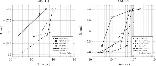
2.4.1 Bound and time comparison of different hierarchies for Example 7 (left) and Example 8 (right). . . 55 2.4.2 Bound and time comparison of different hierarchies for ex2 1 1 (left) and

ex3 1 4 (right). . . 57 2.4.3 Bound and time comparison of different hierarchies for problem (2.7) with

n= 20. . . 61

4.3.1 Comparison of optimal solution of (4.20) for different values of ramping costs r1, r2 (r1= 0, r2 = 0 indicates no ramping costs). . . 97 4.3.2 Unit commodity prices obtained from the solution of (4.20), for different

(12)

Abstract

Historically, polynomials are among the most popular class of functions used for empirical modeling in science and engineering. Polynomials are easy to evaluate, appear naturally in many physical (real-world) systems, and can be used to accurately approximate any smooth function. It is not surprising then, that the task of solving polynomial optimization prob-lems; that is, problems where both the objective function and constraints are multivariate polynomials, is ubiquitous and of enormous interest in these fields. Clearly, polynomial op-timization problems encompass a very general class of non-convex opop-timization problems, including key combinatorial optimization problems.

The focus of the first three chapters of this document is to address the solution of polynomial optimization problems in theory and in practice, using a conic optimization ap-proach. Convex optimization has been well studied to solve quadratic constrained quadratic problems. In the first part, convex relaxations for general polynomial optimization prob-lems are discussed. Instead of using the matrix space to study quadratic programs, we study the convex relaxations for POPs through a lifted tensor space, more specifically, using the completely positive tensor cone and the completely positive semidefinite ten-sor cone. We show that tenten-sor relaxations theoretically yield no-worse global bounds for a class of polynomial optimization problems than relaxation for a QCQP reformulation of the POPs. We also propose an approximation strategy for tensor cones and show empirically the advantage of the tensor relaxation.

(13)

bounds for general polynomial optimization problems. Comparing with other existing SDP and SOCP hierarchies that uses higher degree sum of square (SOS) polynomials and scaled diagonally sum of square polynomials (SDSOS) when the hierarchy level increases, these proposed hierarchies, using fixed degree SOS and SDSOS polynomials but more of these polynomials, perform numerically better. Numerical results show that the hierarchies we proposed have better performance in terms of tightness of the bound and solution time compared with other hierarchies in the literature.

The third chapter deals with Alternating Current Optimal Power Flow problem via a polynomial optimization approach. The Alternating Current Optimal Power Flow (ACOPF) problem is a challenging non-convex optimization problem in power systems. Prior research mainly focuses on using SDP relaxations and SDP-based hierarchies to address the solution of ACOPF problem. In this Chapter, we apply existing SOCP hierarchies to this prob-lem and explore the structure of the network to propose simplified hierarchies for ACOPF problems. Compared with SDP approaches, SOCP approaches are easier to solve and can be used to approximate large scale ACOPF problems.

The last chapter also relates to the use of conic optimization techniques, but in this case to pricing in markets with non-convexities. Indeed, it is an application of conic optimization approach to solve a pricing problem in energy systems. Prior research in energy market pricing mainly focus on linear costs in the objective function. Due to the penetration of renewable energies into the current electricity grid, it is important to consider quadratic costs in the objective function, which reflects the ramping costs for traditional generators. This study address the issue how to find the market clearing prices when considering quadratic costs in the objective function.

(14)

Chapter 1 Convex Relaxations for

Polynomial Optimization

1.1 Introduction

Polynomials appear in a wide variety of areas in science. It is not surprising then that polynomial optimization has recently been a very active field of research [cf., 5]. Here, the interest is the class of non-convex, non-linear POPs. Clearly, a non-convex quadratic program (QP) belongs to this class of problems, and its study has been widely addressed in the literature. For example, to address the solution of QPs, semidefinite programming (SDP) [cf., 113] relaxations have been actively used to find good bounds and approximate solutions for general [see, e.g. 30, 80, 117] and important instances of this problem such as the max-cut problem and the stable set problem (see e.g., [32, 33, 47, 90]). In [58], less computationally expensive second order cone programming (SOCP) [cf., 4] relaxations have also been proposed to approximate non-convex QPs.

The early work linking convex optimization and polynomial optimization in [86, 102] reveals the possibility to use conic optimization to obtain global or near-global solutions for non-convex POPs in which higher than second-order polynomials are used. In the seminal work of Parrilo [89] and Lasserre [66], SDP is used to obtain the global or near-global

(15)

optimum for POPs. Besides SDP approximations, other convex approximations to address the solution of POPs have been investigated using linear programming (LP) and SOCP techniques [2, 67, 68, 91, 121]. These techniques are at the core of the well-known area of Polynomial Optimization [cf., 5].

Alternatively, it has been shown that several NP-hard optimization problems can be expressed as linear programs over the convex cone of copositive matrices and its dual cone, the cone of completely positive matrices, including standard quadratic problems [20], stable set problems [32, 39], graph partitioning problems [93], and quadratic assignment prob-lems [94]. In [27], Burer shows the much more general result that every quadratic problem with linear and binary constraints can be rewritten as such a problem. Completely positive relaxations for general quadratically constrained quadratic programs (QCQPs) have been studied in [8, 29]. In [11], CP reformulation for QCQPs and quadratic program with com-plementarity constraints (QPCCs) are discussed without any assumptions on the feasible regions. Although copositive/completely positive cones are not tractable in general, recent advances on obtaining algorithms ([3, 26, 35], etc.) to approximate copositive/completely positive cones provide an alternative way to globally solve quadratic POPs. Recently, Bomze shows in [18] that copositive relaxation provides stronger bounds than Lagrangian dual bounds in quadratically and linearly constrained QPs.

A natural thought is whether one can extend the copositive programming or completely positive programming reformulations for QPs to POPs. In [9], Arima et al. proposed the moment cone relaxation for a class of polynomial optimization problems (POPs) to extend the results on the completely positive cone programming relaxation for the quadratic optimization. Recently, Pena et al. show in [92] that under certain conditions general POPs can be reformulated as a conic program over the cone of completely positive tensors, which is a natural extension of the cone of completely positive matrices in quadratic problems. This tensor representation was originally proposed in [38], and is now the focus of active research [see, e.g., 53, 56, 78, 106]. In [92], it is also shown that the conditions for the equivalence of POPs and the completely positive conic programs, when applied to QPs,

(16)

lead to conditions that are weaker than the ones introduced in [27].

In [64], we study completely positive (CP) and completely positive semidefinite (CPSD) tensor relaxations for POPs. Our main contributions are: 1) We extend the results for QPs in [18] to general POPs by using CP and CPSD tensor cones. In particular, we show that CP tensor relaxations provide tighter bounds than Lagrangian relaxations for general POPs. 2) We provide tractable approximations for CP and CPSD tensor cones that can be used to globally approximate general POPs. 3) We prove that CP and CPSD tensor relaxations yield tighter bounds than completely positive and positive semidefinite matrix relaxations for quadratic reformulations of some classes of POPs. 4) We provide preliminary numerical results on more general cases of POPs and show that the approx-imation of CP tensor cone programs can yield tighter bounds than relaxations based on doubly nonnegative (DNN) matrices [cf., 14] for completely positive matrix relaxation to the reformulated quadratic programs.

The remainder of the chapter is organized as follows. We briefly introduce the basic con-cepts of tensor cone and tensor representation of polynomials in Section 1.2. Lagrangian, completely positive semidefinite tensor, and completely positive tensor relaxations for PO problems are discussed in Section 1.3. In Section 1.4, we discuss a quadratic approach to general POPs; that is, when auxiliary decision variables are introduced to the problem to reformulate it as a Quadratically Constrained Quadratic Program (QCQP). Then, the completely positive relaxations is applied to the resulting QCQPs and the bounds are com-pared with those obtained from the tensor relaxations for a class of POPs. In Section 1.5, Linear Matrix Inequality (LMI) approximation strategies for the positive semidefinite and completely positive tensor cones are developed and a comparison of tensor relaxations with matrix relaxations obtaining using the quadratic approach is done by obtaining numerical results on several POPs. Lastly, Section 1.6 summarizes the results and provides future working directions.

(17)

1.2 Preliminaries

1.2.1 Basic Concepts and Notations

We first introduce basic concepts and notations used throughout the chapter. Follow-ing [92], we start by definFollow-ing tensors.

Definition 1. Let _Tn,d denote the set of tensors of dimension n and order d in Rn, that is

Tn,d =Rn⊗ · · · ⊗Rn

| {z }

d

,

where ⊗ is the tensor product.

A tensor T _{⊆ T}n,d is symmetric if the entries are independent of the permutation of its indices. We denote Sn,d⊆ Tn,d as the set of symmetric tensors of dimension n and order

d. For anyT1, T2∈ Tn,d, let h·,·in,d denote the tensor inner product defined by

hT1, T2_in,d= X {i1,...,id}∈{1,...,n}d T₍1_i₁_,...,i d)T 2 (i1,...,id).

Definition 2. For any x∈Rn, let the mapping Rn→ Sn,d be defined by

Md(x) =x⊗ · · · ⊗x

| {z }

d

.

Definition 1 and 2 are natural extensions of matrix notations to higher order. For example, _Tn,2 is the set n×nmatrices, while Sn,2 is the set ofn×nsymmetric matrices,

h·,_·in,2 is the Frobenius inner product andM2(x) =xxT for anyx∈Rn. In general,Md(x) is the symmetric tensor whose (i1, ..., id) entry isxi1· · ·xid.

Proposition 1. Let En,d be all 1 tensor with dimension n and order dand e∈Rn be the all one vector, then

(18)

Proof. By the definition of Md(·) andh·,·in,d, hEn,d, Md(x)in,d= X k1+k2+···+kn=d d k1, k2, . . . , kn xk1 1 xk22· · ·xnkn = (eTx)d, where _k d 1,k2,...,kn

is the multinomial coefficient.

Proposition 2. Forx_∈Rn, y∈Rn,

hMd(x), Md(y)in,d= (xTy)d.

Proof. Let x, y _∈ Rn be given and z ∈ Rn be defined as zi = xiyi, i = 1, ..., n, and let

e_∈Rn be the all one vector, from the definition ofMd(·) andh·,·in,d,

hMd(x), Md(y)in,d= X {i1,...,id}∈{1,...,n}d Md(x)(i1,...,id)Md(y)(i1,...,id) = X {i1,...,id}∈{1,...,n}d xi1xi2· · ·xid·yi1yi2· · ·yid = X {i1,...,id}∈{1,...,n}d (xi1yi1)(xi2yi2)· · ·(xidyid) =_hEn,d, Md(z)in,d = (eTz)d (from Proposition 1) = (xTy)d.

Analogous to positive semidefinite and copositive matrices of order 2, positive semidef-inite and copositive tensors can be defined as follows.

Definition 3. Define the _K-semidefinite (or set-semidefinite) symmetric tensor cone of dimension nand order d as:

(19)

For _K =Rn, Cn,d(Rn) denotes the positive semidefinite (PSD) tensor cone. For K=Rn+,

Cn,d(Rn+) denotes the copositive tensor cone.

Similar to the one-to-one correspondence of n×n PSD matrices to nonnegative ho-mogeneous quadratic polynomials ofnvariables, there is also a one-to-one correspondence of PSD tensors with dimension n and order d to nonnegative homogeneous polynomials with n variables and degree d [cf., 78]. Note that there is no nonnegative homogeneous polynomial with odd degree. Thus it follows that there is no PSD tensor with odd order. Next we discuss the dual cones of _Cn,d(Rn+) and Cn,d(Rn), following the discussion in [78] and [92].

Definition 4. Given any cone _C of symmetric tensors, the dual cone of _C is

C∗=_{Y _{∈ S}n,d:hX, Yi ≥0,∀X ∈ C},

and if _C∗ =_C, then cone _C is self-dual.

The dual cones of the positive semidefinite tensor cone and copositive tensor cone have been studied in [78] and [92]. More formally,

Proposition 3.

(a) _C_n,d∗ (Rn+) = conv{Md(x) :x∈Rn+}.

(b) C∗

n,2d(Rn) = conv{M2d(x) :x∈Rn}.

Similar to the completely positive matrix coneC∗

n,2(Rn+), we callCn,d∗ (Rn+) thecompletely

positive (CP) tensor cone. It is well known that the positive semidefinite matrix cone is self-dual, however, in general, the positive semidefinite tensor cone is not self-dual [cf., 78]. Thus, here we name _C∗

n,2d(Rn) as the completely positive semidefinite (CPSD) tensor cone. Before formally stating that_C∗

n,2d(Rn)=6 Cn,2d(Rn) in general, we first introduce the homogeneous sum of square (SOS) tensor cone of dimensiondand order 2das

Cn,2d(SOS) ={Tn,2d:hTn,2d, M2d(x)i= X i λi hTn,di , Md(x)i 2 , f or some λi ≥0}.

(20)

Similarly, there is a one-to-one corresponding relationship between homogeneous SOS ten-sors with dimensionn and order 2dand homogeneous SOS polynomials with dimension n and degree 2d. Next we discuss the relationships between nonnegative and sum of square polynomials from the perspective of tensor representation and reveal the relationship be-tween SOS and CPSD tensors.

Proposition 4 ([78, Prop. 5.8 (i)]).

Cn,∗2d(Rn)⊆ Cn,2d(SOS)⊆ Cn,2d(Rn). Proof. Let T _{∈ C}∗ n,2d(Rn), by Proposition 3,T = P iλiM2d(yi), yi ∈Rn, λi≥0, P iλi = 1. Then _∀x_∈Rn, hT, M2d(x)in,2d= * X i λiM2d(yi), M2d(x) + n,2d =X i λiM2d(yi), M2d(x)_n,₂_d =X i λi(xTyi)2d (from Proposition 2) =X i hp λi(xTyi)d i2 .

Take z_ki =xkyi_k, then xTyi=eTzi wheree∈Rnis an all one vector. Therefore,

hT, M2d(x)in,2d= X i hp λi(eTzi)d i2 =X i hp λihEn,d, Md(zi)in,d i2 , (from Proposition 1) therefore C∗

n,2d(Rn) ⊆ Cn,2d(SOS). By the definition of homogeneous SOS tensor cone, it is clear that_Cn,2d(SOS)⊆ Cn,2d(Rn).

The proof of Proposition 4 can be seen as an alternative proof for Proposition 5.8 (i) in [78] using the tensor notations introduced here. Well studied sum of square polynomial

(21)

optimization reveals that a nonnegative multivariate homogeneous polynomial is a homoge-neous sum of square polynomial if it is quadratic, that is_C∗

n,2(Rn) =Cn,2(SOS) =Cn,2(Rn). This statement coincides with the self-duality of the PSD matrix cone. Luo et al. showed in [78] that _C∗

n,2d(Rn) ( Cn,2d(SOS) for d≥2. On the other hand, the Motzkin polyno-mial together with isomorphism between homogeneous polynopolyno-mials and tensors shows that

Cn,2d(SOS)(Cn,2d(Rn) whend≥2.

1.2.2 Tensor Representation of Polynomial Optimization

In section 1.2.1, we discussed that some homogeneous polynomials can be expressed as tensor inner product with Md(x). Next, we introduce a tensor representation for general polynomials that are not necessarily homogeneous. DefineR[x] as the ring of polynomials with real coefficients in Rn, and let Rd[x] := {p ∈ R[x] : deg(p) ≤ d} denote the set of polynomials with dimensionnand degree at mostd. For simplicity, we useMd(1, x), x∈Rn to represent Md((1, xT)T), x ∈ Rn throughout this paper. For any p(x) ∈ Rd[x], we can write p(x) as

p(x) =_hTd(p), Md(1, x)in+1,d, (1.1)

whereTd(·) is the mapping of coefficients ofp(x) in terms ofMd(1, x) inSn+1,d. Following [92], define Td:Rd[x]→ Sn+1,d as Td   X β∈_Zn +:|β|≤d pβxβ   i1,...,id := α1!· · ·αn! |α|! pα,

where α is the (unique) exponent such that xα _:= _xα1

1 · · ·xαnn = xi1· · ·xid (i.e., αk is

the number of times k appears in the multi-set _{i1, . . . , id}) and |α|= Pni=1αi. For any polynomial p(x)_∈Rd[x], let ˜p(x) denote the homogenous component ofp(x) with highest degree, then it follows

˜

(22)

Equation (1.1) and (1.2) allow us to represent any multivariate polynomials with their tensor forms and provide the possibility to study the boundedness of general polynomials with their tensor representations.

Theorem 1. Let µ∈R, we have

(a) Letp(x)∈Rd[x]. Thenp(x)≥µfor allx∈Rn+if and only ifTd(p−µ)∈ Cn+1,d(Rn++1).

(b) Let p(x) _∈ R2d[x]. Then p(x) ≥ µ for all x ∈ Rn if and only if T2d(p −µ) ∈

Cn+1,2d(Rn+1).

Proof. For (a), assumeTd(p−µ)∈ Cn+1,d(Rn++1). By Definition 3,hTd(p−µ), Md(1, x)in+1,d≥ 0,_∀x_∈Rn+, then

p(x)−µ=hTd(p−µ), Md(1, x)in+1,d≥0, ∀x∈Rn+. (1.3)

For the other direction, assumep(x)_≥µ,_∀x_∈Rn+, then by (1.3),hTd(p−µ), Md(1, x)in+1,d ≥ 0,_∀x_∈Rn+. Thus, for any (x0, x)∈R++×Rn+,

hTd(p−µ), Md(x0, x)in+1,d=x0hTd(p−µ), Md(1,

x

x0)in+1,d≥0. (1.4)

Furthermore, due to continuity, for k >0,

hTd(p−µ), Md(0, x)i= lim

k→+∞hTd(p−µ), Md(1/k, x)i ≥0, (1.5)

where the last inequality follows from (1.4). From (1.4), (1.5), and Definition 3, it follows thatTd(p−µ)∈ Cn+1,d(Rn++1).

The proof of (b) is similar to the proof of (a).

Corollary 1. Let µ_∈R, we have

(a) Let p(x)∈Rd[x]. Then inf{p(x) :x∈Rn+}= sup{µ∈R:Td(p−µ)∈ Cn+1,d(Rn++1)}.

(23)

Theorem 1 and Corollary 1 generalize the key Lemma 2.1 and Corollary 2.1 in [18] for polynomials with degree higher than two using tensor representation. Moreover, Corollary 1 can be seen as a convexification of an unconstrained (possibly non-linear non-convex) POP to a linear conic program over CP and CSDP tensor cones. In the next section, we will discuss the convex relaxations for general constrained polynomial optimization problems.

1.3 Relaxations of POPs

Letpi∈Rd[x], i= 0, . . . , m. Consider two general POPs with polynomial constraints:

z+ = inf p0(x) s.t. pi(x)≤0, i= 1, . . . , m x_∈Rn+, (1.6) and z= inf p0(x) s.t. pi(x)≤0, i= 1, . . . , m, (1.7)

where d = max{deg(pi) : i ∈ {0,1, . . . , m}}. Problems (1.6) and (1.7) represent general POPs, which encompass a large class of linear convex problems, including non-convex QPs with binary variables (i.e., binary constraints can be written in the polynomial form xi(1−xi) ≤ 0, −xi(1−xi) ≤ 0). Naturally, we have z ≤ z+ since the feasible set of problem (1.6) is a subset of problem (1.7). Next we show that the results of Bomze for quadratic problems [18] can be extended to POPs of form (1.6) and (1.7).

1.3.1 Lagrangian relaxations

Let ui ≥ 0 be the Lagrangian multiplier of the inequality constraints pi(x) ≤ 0 for i = 1, .., m and vi ≥ 0 for constraintsxi ∈ R+ for i= 1, ..., n, so the Lagrangian function for

(24)

problem (1.6) is L+(x;u, v) :=p0(x) + m X i=1 uipi(x)−vTx,

so the Lagrangian dual function of problem (1.6) is

Θ+(u, v) := inf{L+(x;u, v) :x∈Rn},

with its optimal value

zLD,+= sup{Θ+(u, v) : (u, v)∈Rm+ ×Rn+},

We also use a Semi-Lagrangian dual function to represent the nonnegative variable constraints of problem (1.6),

Θsemi(u) := inf{L(x;u) :x∈Rn+},

with its optimal value

zsemi= sup{Θsemi(u) :u∈Rm+},

Similarly, letui ≥0 be the Lagrangian multiplier of the inequality constraintspi(x)≤0 fori= 1, ..., m, so the Lagrangian function for problem (1.7) is

L(x;u) :=p0(x) +

m

X

i=1

uipi(x),

so the Lagrangian dual function of problem (1.7) is

Θ(u) := inf_{L(x;u) :x_∈Rn},

and the dual optimal value is

(25)

from weak duality theory, we havezLD ≤z. Thus we have the following relationship:

Θ+(u, v) = inf{L+(x;u, v) :x∈Rn}

≤inf_{L+(x;u, v) :x∈Rn+} = inf{L(x;u)−vTx:x∈Rn+}

≤inf_{L(x;u) :x_∈Rn+}= Θsemi(u),

where the second inequality holds because x, v _∈Rn+ always implies vTx ≥ 0. Therefore, we have:

zLD,+≤zsemi ≤z+, where the latter inequality holds by weak duality.

1.3.2 CPSD tensor relaxation for free variables

Consider followingconic program:

zSP = inf hTd(p0), Xi

s.t. _hTd(pi), Xi ≤0, i= 1, . . . , m

hTd(1), Xi= 1

X_{∈ C}_n∗₊₁_,d(Rn+1),

(1.8)

and its conic dual problem is

zSD = sup{µ:Td(p0)−µTd(1) + m

X

i=1

uiTd(pi)∈ Cn+1,d(Rn+1), u∈Rm+}. (1.9)

For simplicity, we use _h·,_·i represent the tensor inner product of appropriate dimension and order.

Proposition 5. Problem (1.8) is a relaxation of problem (1.7) withzSP ≤z.

(26)

a feasible solution of problem (1.8) directly by applying (1.1). Also p(x) = hTd(p0), Xi is a direct result of (1.1) with the same objective value.

Theorem 2. For problem (1.7), its Lagrangian dual function optimal value satisfies,

zLD = sup{µ: (µ, u)∈R×Rm+, Td(L(x;u)−µ)∈ Cn+1,d(Rn+1)} and zLD =zSD≤zSP ≤z. Proof. By Corollary 1 (b), Θ(u) = inf_{L(x;u) :x_∈Rn} = sup{µ:Td(L(x;u)−µ)∈ Cn+1,d(Rn+1)}, then zLD= sup{Θ(u) :u∈Rm+} = sup_{µ: (µ, u)_∈R×Rm+, Td(L(x;u)−µ)∈ Cn+1,d(Rn+1)}. From (1.9), we have zSD = sup{µ:Td(p0)−µTd(1) + m X i=1 uiTd(pi)∈ Cn+1,d(Rn+1), u∈Rm+} = sup{µ:Td(p0+ m X i=1 uipi−µ)∈ Cn+1,d(Rn+1), u∈Rm+} = sup{Θ(u) :u∈Rm+} =zLD.

Furthermore,zSD ≤zSP ≤zholds directly from weak conic duality and Proposition 5.

From Theorem 2, the Lagrangian dual optimal value has no duality gap if and only if conic program itself has no duality gap and positive semidefinite tensor relaxation is tight.

(27)

1.3.3 CP and CPSD tensor relaxations for nonnegative variables Consider followingconic programs:

zCP = inf hTd(p0), Xi s.t. hTd(pi), Xi ≤0, i= 1, . . . , m hTd(1), Xi= 1 X_{∈ C}_n∗₊₁_,d(Rn++1), (1.10) and zSP,+= inf hTd(p0), Xi s.t. hTd(pi), Xi ≤0, i= 1, . . . , m hTd(−xi), Xi ≤0, i= 1, . . . , n hTd(1), Xi= 1 X ∈ Cn∗+1,d(Rn+1), (1.11)

and their conic dual problems

zCD = sup{µ:Td(p0)−µTd(1) + m X i=1 uiTd(pi)∈ Cn+1,d(Rn++1), u∈Rm+}. (1.12) zSD,+= sup{µ:Td(p0−µ)+ m X i=1 uiTd(pi)+ n X i=1 viTd(−xi)∈ Cn+1,d(Rn+1), u∈Rm+, v∈Rn+}. (1.13)

Proposition 6. Problem (1.10)and problem (1.11)are relaxations for problem (1.6)with

zCP ≤z+ and zSP,+≤z+.

Theorem 3. For problem (1.6), its Semi-Lagrangian dual function optimal value and its Lagrangian dual function optimal value satisfy

zsemi = sup{µ: (µ, u)∈R×Rm+, Td(L(x;u)−µ)∈ Cn+1,d(Rn++1)},

(28)

and (a) zLD,+≤zsemi=zCD ≤zCP ≤z+. (b) zLD,+=zSD,+ ≤zSP,+≤z+. Proof. By Corollary 1, Θsemi(u) = inf{L(x;u) :x∈Rn} = sup_{µ:Td(L+(x;u)−µ)∈ Cn+1,d(Rn+1)}, Θ+(u, v) = inf{L+(x;u, v) :x∈Rn} = sup_{µ:Td(L+(x;u, v)−µ)∈ Cn+1,d(Rn+1)}, then

zsemi = sup{Θsemi(u) :u∈Rm+}

= sup{µ: (µ, u)∈R, Td(L(x;u)−µ)∈ Cn+1,d(Rn++1)}. zLD,+= sup{Θ+(u, v) :u∈Rm+, v∈Rn+}

= sup_{µ: (µ, u, v)_∈R×Rm+ ×Rn, Td(L+(x;u, v)−µ)∈ Cn+1,d(Rn+1)}.

For (a), from (1.12), we have,

zCD = sup{µ:Td(p0)−µTd(1) + m X i=1 uiTd(pi)∈ Cn+1,d(Rn++1), u∈Rm+} = sup{µ:Td(p0(x) + m X i=1 uipi(x)−µ)∈ Cn+1,d(Rn++1), u∈Rm+} = sup{µ: (µ, u)∈R×Rm+, Td(L(x;u)−µ)∈ Cn+1,d(Rn++1)} = sup_{Θsemi(u) :u∈Rm+} =zsemi.

(29)

(b), from (1.13), we have zSD,+= sup{µ:Td(p0−µ) + m X i=1 uiTd(pi) + n X i=1 viTd(−xi)∈ Cn+1,d(Rn+1), u∈Rm+, v∈Rn+} = sup_{µ:Td(p0(x) + m X i=1 uipi(x)− n X i=1 vTx₋µ)_{∈ C}n+1,d(Rn+1), u∈Rm+, v ∈Rn+} = sup{µ: (µ, u, v)∈R×Rm+×Rn+, Td(L+(x;u, v)−µ)∈ Cn+1,d(Rn+1)} = sup_{Θ+(u, v) :u∈Rm+, v∈Rn+} =zLD,+.

And zSD,+≤zSP,+≤z+ holds directly from weak conic duality and Proposition 6.

1.4 Quadratic Reformulation for POPs and its Relaxations

Section 1.3 showed that CP and CPSD tensor relaxations are tighter than Lagrangian relax-ations for general POPs. In this section, we will compare CP and CPSD tensor relaxrelax-ations with quadratic approach for POPs. For general POPs, a classic approach to obtain relax-ations is to reformulate them as quadratic programs by introducing additional variables and constraints to address the higher degree terms in polynomials. And a well-studied SDP relaxation or CP relaxation on quadratic constrained quadratic program (QCQP) can then be applied to the reformulated QCQP. Also as discussed in this paper, general POPs can be relaxed directly by conic programs over the CP or the CPSD tensor cones. In general, it is difficult to compare these two relaxations. In this section, we will focus on POPs with degree 4 and apply these two relaxations and show some specific cases in which tensor cone relaxations of POPs give tighter bounds than convex relaxations of QCQP reformulation of POPs.

(30)

1.4.1 QCQP Reformulation of POP

A general QCQP reformulation technique of POPs, including how to add additional vari-ables, is discussed in [92]. In this section, the main focus is on some classes of 4th degree POPs, so we use a specific reformulation approach here. We will introduce additional variables to represent the quadratic terms (i.e. the square of single variable and the mul-tiplication of two variables) of the original variables. Consider the following POPs:

sup p0(x)

s.t. pi(x)≤di, i= 1, . . . , m0, qj(x)≤0, j = 1, . . . , m1, x∈Rn+,

(1.14)

where p0(x) ∈ R4[x], qj ∈ R2[x] (Recall Rd[x] := {p ∈ R[x] : deg(p) ≤ d}) and pi(x) are homogeneous polynomials of degree 4. Problem (1.14) can encompass a large class of 4th degree optimization problems, including problem with 4th degree objective function and linear/quadratic(binary) constraints and so on. This type of optimization problems also appears in many real life problems, such as biquadratic assignment problem [81, 96], Alternating Current Optimal Power Flow (ACOPF) problem [22, 44, 65, 71], etc.

Define an index set

S ={(a, b, c)∈N3 :a= 1, . . . , n, b=a, . . . , n, c= (n+ 1−a

2)(a−1) +b−a+ 1} (1.15)

as the index for the additional variables, so that it is from 1 to _|S_| = n+1₂

, which is the maximum number of additional variables needed to reformulate 4th degree polyno-mials using 2nd degree polynopolyno-mials. Specifically, introducing additional variables yc =

(31)

xaxb,∀(a, b, c)∈S, the QCQP reformulation of problem (1.14) can be represented as sup q0(x, y) s.t. hi(y)≤di, i= 1, . . . , m0, qj(x)≤0, j = 1, . . . , m1, yc−xaxb = 0,∀(a, b, c)∈S, x_∈Rn+, y∈R |S| + , (1.16)

whereq0(x, y) andhi(y) are the reformulated quadratic polynomials with original variables

x and additional variables y by replacingxaxb with yc,∀(a, b, c) ∈S, note that hi(y) are homogeneous polynomials of degree 2. It is clear that p0(x) =q0(x, y), pi(x) =hi(y), i = 1, . . . , m0, therefore problem (1.14) and (1.16) are equivalent. As pi(x) and hi(y) are homogeneous polynomials, then it follows that

˜

pi(x) =pi(x) =hi(y) = ˜hi(y), i= 1, . . . , m0. (1.17)

To make the formula clear and easy to represent in a conic program, letz= (x, y)_∈Rn++|S|, then (1.16) is equivalent to sup q0(z) s.t. hi(z)≤di, i= 1, . . . , m0, qj(z)≤0, j = 1, . . . , m1, zn+c−zazb = 0,∀(a, b, c)∈S, z∈Rn++|S|. (1.18) Example 1. QP Reformulation

(32)

Consider the following univariate program, sup x4+x3+x2+x+ 1 s.t. x4_≤1, x2−x−2≤0, −x+ 1_≤0, x_∈R+. (1.19)

Lety=x2 andz= (x, y)_∈R2+, then problem (1.19) is equivalent to

sup y2+xy+y+x+ 1 sup z₂2+z1z2+z2+z1+ 1 s.t. y2 ≤1, s.t. z2 ≤1,

y₋x₋2_≤0, _≡ z2−z1−2≤0,

−x+ 1_≤0, ₋z1+ 1≤0, x∈R+, y ∈R+. z∈R2+.

1.4.2 CP matrix relaxations for QCQP

Consider the following CP matrix relaxations for problem (1.18),

sup hT2(q0(z)), Zi s.t. _hT2(hi(z)), Zi ≤di, i= 1, . . . , m0, hT2(qj(z)), Zi ≤0, j = 1, . . . , m1, hT2(1), Zi= 1, Z1,n+c+1−Za+1,b+1= 0,∀(a, b, c)∈S, Z ∈ Cn∗+r+1,2(Rn++r+1). (1.20)

where r = _|S_| is the number of additional variables in problem (1.18). Problem (1.20) is a natural CP tensor relaxation of problem (1.18) and by relaxing the equality constraints

(33)

Z1,c+n+1 −Za+1,b+1 = 0,∀(a, b, c) ∈ S into inequality constraints, we have the following CP tensor relaxation, sup hTd(q0(z)), Zi s.t. _hT2(hi(z)), Zi ≤di, i= 1, . . . , m0, hT2(qj(z)), Zi ≤0, j = 1, . . . , m1, hT2(1), Zi= 1, Z1,c+n+1−Za+1,b+1≤0,∀(a, b, c)∈S, Z ∈ Cn∗+r+1,2(Rn++r+1), (1.21)

Proposition 7. If problem (1.20)is feasible and the coefficients ofq0(z) in problem (1.20)

are nonnegative, then problems (1.20) and (1.21)are equivalent.

Proof. It is clear that if the coefficients of objective function q0(z) are nonnegative, at optimality of problem (1.21), Z1,k+n+1 =Zi+1,j+1 holds. And the same objective function values are obtained for problems (1.20) and (1.21).

Recall the CP tensor relaxation (1.10) for general POPs and apply it directly to prob-lem (1.18), then we have the following conic program,

sup _hTd(p0(x)), Xi s.t. hTd(pi(x)), Xi ≤di, i= 1, . . . , m0, hTd(qj(x)), Xi ≤0, j = 1, . . . , m1, hTd(1), Xi= 1, X∈ Cn∗+1,d(Rn++1), (1.22)

Problem (1.20) and (1.22) can be seen as two different relaxations for some classes POPs with a form of problem (1.14). Problem (1.20) characterizes the polynomials with higher degree than 2 by reformulating them as quadratic polynomials. SDP and CP matrix relaxations for the reformulated QCQP are well studied in literature [cf., 5, 18, 19, 20,

(34)

27, 29, 58, 113]. However, the introduce of additional constraints Z1,c+n+1−Za+1,b+1 = 0,_∀(a, b, c) _∈ S in problem (1.20) may ruin some exact relaxation conditions for QCQP. Problem (1.22) characterizes the polynomials with degree higher than 2 by using higher order tensors which avoids introducing additional variables and constraints. Next we will show that under some conditions, the latter relaxations will provide tighter bounds for problem (1.14).

Lemma 1 ([92, Lemma 2]). For any d >0 and n >0, _C_n∗₊₁_,d(Rn++1) =conic(Md({0,1} × Rn+)).

Theorem 4. Consider a feasible problem (1.14) where the coefficients of p0(x) are non-negative, then problem (1.20) is a relaxation of problem (1.22).

Proof. By Proposition 7, problems (1.20) and (1.21) are equivalent. For any feasible solu-tion X∈ C∗ n+1,4(Rn++1) to problem (1.22), by Lemma 1, X= n1 X s=1 λsM4(1, us) + n0 X t=1 γtM4(0, vt),

for somen0, n1 ≥0, λs, γt>0 and us, vt∈Rn+. Then by using (1.1),

1 =_hT4(1), Xi= n1 X s=1 λs, di ≥ hT4(pi), Xi= n1 X s=1 λspi(us) + n0 X t=1 γtp˜i(vt), i= 1, ..., m0, 0_{≥ h}T4(qj), Xi= n1 X s=1 λsqj(us) + n0 X t=1 γtq˜j(vt), j = 1, ..., m1, (1.23)

with an objective function value ofPn₁

s=1λsp0(us) +Pnt=10 γtp˜0(vt). Recall the index set S in (1.15), and construct a vector ofws,wt0 fors= 1, ..., n1, t= 1, ..., n0 as follows:

(ws)c= (us)a(us)b, (a, b, c)∈S, (w0_t)c= (vt)a(vt)b, (a, b, c)∈S.

(35)

Next we show Z = n1 X s=1 λsM2(1,(us, ws)) + n0 X t=1 γtM2(0,(vt, w0t)), (1.25)

is a feasible solution to problem (1.20). Clearly, Z _{∈ C}∗

n+r+1,2(Rn++r+1), and from equa-tion (1.24) and (1.25), we have

Z1,c+n+1= n1 X s=1 λs(ws)c= n1 X s=1 λs(us)a(us)b,∀(a, b, c)∈S, Za+1,b+1= n1 X s=1 λs(us)a(us)b+ n0 X t=1 γt(vt)a(vt)b,∀(a, b, c)∈S,

which indicates thatZ1,c+n+1 ≤Za+1,b+1, ∀(a, b, c)∈S. From equations (1.17) and (1.23),

hT2(1), Zi= n1 X s=1 λs= 1, hT2(hi), Zi= n1 X s=1 λshi(ws) + n0 X t=1 γt˜hi(wt0) = n1 X s=1 λspi(us) + n0 X t=1 γtp˜i(vt)≤di, i= 1, ..., m0, hT2(qj), Zi= n1 X s=1 λsqj(us) + n0 X t=1 γtq˜j(vt)≤0, j = 1, ..., m1,

with an objective value of n1 X s=1 λsq0(us, ws) + n0 X t=1 γtq˜0(vt, w0t) = n1 X s=1 λsp0(us) + n0 X t=1 γtq˜0(vt, w0t),

under the condition that p0(x) has nonnegative coefficients andx∈Rn+,

n0 X t=1 γtq0˜(vt, wt0)≥ n0 X t=1 γtp0˜ (vt).

Therefore, from any feasible solution to problem (1.22), we can construct a feasible solution to problem (1.21) with a larger objective function value, which indicates that problem (1.20) is a relaxation for problem (1.22).

(36)

Theorem 4 illustrates that theoretically the CP tensor relaxation can provide tighter bounds than QCQP approches for a class of POPs. In next section, we will introduce some approximation strategies for CP and CPSD tensor programs to address the intractability.

1.5 Numerical Comparison of Two Relaxations of PO

Unlike the tractability of the PSD matrix cone, the CPSD tensor cone is not tractable in general to our knowledge. Also similar to the intractability of completely positive matrices of dimension greater than 5, the CP tensor cone is also not tractable in general. In this section, we will discuss and develop tractable approximations for CP and CPSD tensor cones, and then use these approximations to address some POPs to show it provides better bounds than approximations for QCQP reformulation.

1.5.1 Approximation of CP and CPSD Tensor Cones

Before presenting results, let us introduce some more notations. For T =Md(x), x∈Rn, denoteT₍_i₁_,...,i_d₎as the element in (i1, ..., id) position, where (i1, ..., id)∈ {1, . . . , n}d. To be more specific,ij withj= 1, ..., dmeans the choice of{x1, ..., xn} in thejth position in the tensor product, i.e. i1 = 2 means choosing x2 as the first position in the tensor product. To illustrate, let x∈R3 and let

T1 =M2(x) =       x2₁ x1x2 x1x3 x1x2 x22 x2x3 x1x3 x2x3 x23       , thenT1

(1,2)=x1x2 and it is in the (1,2) position in T1. Also forT =Md(x), x∈Rn, when d >2, letT₍_i₁_,...,i_d₋₂_,·,·) denote the matrix in (i1, ..., id−2,·,·) position, where (i1, ..., id−2,·,·) represents the matrix

(37)

for example, letT2 =M3(x), x∈R3, then T₍₁2_,_·_,_·₎=       x3₁ x2₁x2 x21x3 x2₁x2 x1x2₂ x1x2x3 x2₁x3 x1x2x3 x1x2₃       , T₍₂2_,_·_,_·₎=       x2₁x2 x1x22 x1x2x3 x1x2₂ x3₂ x2₂x3 x1x2x3 x2₂x3 x2x2₃       .

Definition 5. LetT =Md(x), x∈Rn. For any(i1, . . . , id−2)∈ {1, . . . , n}d−2,T(i1,...,id−2,·,·) is a principal matrix if Ik ⊆ {0, . . . , d−2} is even for all k = 1, . . . , n, where Ik is an ordered set of the number of appearance ij =k,∀j= 1, . . . , d−2 where k= 1, ..., n.

For example, let T3 =M8(x), x∈R3, then

T₍₁3_,₁_,₂_,₂_,₃_,₃_,_·_,_·₎, T₍₁3_,₂_,₂_,₂_,₁_,₂_,_·_,_·₎, T₍₂3_,₃_,₂_,₁_,₃_,₁_,_·_,_·₎ are principal matrices; T₍₁3_,₁_,₁_,₂_,₃_,₃_,_·_,_·₎, T₍₁3_,₂_,₂_,₂_,₂_,₂_,_·_,_·₎, T₍₂3_,₃_,₂_,₂_,₃_,₁_,_·_,_·₎ are not principal matrices.

Notice the symmetry of symmetric tensors, T(i1,...,id−2,·,·) with the sameIk, k= 1, ..., n are equal. Next we will discuss the approximation strategies for the CP and the CPSD tensor cones based on PSD and DNN matrices.

Definition 6. A symmetric matrix X is called doubly nonnegative (DNN) if and only if

X0 andX ≥0, where X ≥0 indicates every element of X is nonnegative.

Proposition 8. For any symmetric tensorT,

(a) If T _{∈ C}∗

n,d(Rn+), then T(i1,...,id)≥0, T(i1,...,id−2,·,·)0,∀i= 1, ..., n. (b) If T ∈ C∗

n,d(Rn), for all principal matrices T(i1,...,id−2,·,·), T(i1,...,id−2,·,·) 0,∀i= 1, ..., n. Proof. For part (a), by Proposition 3 (a),T =P

iλiMd(xi), wherexi ∈Rn+, λi ≥0,Piλi = 1, then it is clear that T₍_i₁_,...,i_d₎ _≥0, and

T(i1,...,id−2,·,·)= X i λi n Y k=1 (xi_k)Ik₍_xi₍_xi₎T₎_, _(1.26)

(38)

asxi(xi)T 0,∀iand Qn

k=1(xik)Ik ≥0, then T(i1,...,id−2,·,·) 0. For part (b), noticing that the number of appearanceIk, k= 1, ..., nis even ifT(i1,...,id−2,·,·) is a principal matrix, then it follows proof of (a) withQn

k=1(xik)Ik ≥0 in (1.26). Take T ∈ C∗

2,4(R2+) as an example to illustrate Proposition 8, by Proposition 3 (a), T =P

iλiM4(xi), where λi ≥0,

P

iλi = 1 and xi ∈R2+, then for anyy∈R2,

yTT₍₁_,₂_,·,·)y =yT X i λiM4(xi)(1,2,·,·)y=xi1xi2 X i (yTxi)2_≥0,

which indicates that T(1,2,·,·) is a 2×2 positive semidefinite matrix.

Next we discuss the approximation of the CPSD and the CP tensor cones. Based on Proposition 8, we define the following tensor cones,

KSDPn,d ={T ∈ Sn,d:T(i1,...,id−2,·,·)0, ∀(i1, . . . , id−2)∈ {1, . . . , n} d−2_}_, Kn,dL ={T ∈ Sn,d:T(i1,...,id) ≥0, ∀(i1, . . . , id)∈ {1, . . . , n} d }, Kn,dDN N ={T ∈ Sn,d:T(i1,...,id−2,·,·)0, T(i1,...,id−2,·,·)≥0, ∀(i1, . . . , id−2)∈ {1, . . . , n} d−2_}_. It is easy to see these cones are convex closed cones with the following relationship,

Cn,d∗ (Rn)⊆ KSDPn,d

Cn,d∗ (Rn+)⊆ KDN Nn,d ⊆ Kn,dL .

(1.27)

Consider the following conic program,

[TP-K] inf hTd(p0), Xi

s.t. _hTd(pi), Xi ≤0, i= 1, . . . , m

hTd(1), Xi= 1

X _{∈ K}n+1,d.

(39)

choosing appropriate tractable cones, and thus provides relaxations to globally approximate general POPs. It follows that

z_[TP-_KSDP_] ≤z_SP ≤z,

z_[TP-_KL_] ≤z_[TP-_KDN N_] ≤z_CP ≤z₊.

1.5.2 Numerical results on general cases

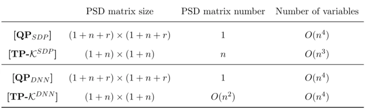
In Section 1.5.1, several tractable approximations for the CP and the CPSD tensor cones have been developed to provide relaxations for CP and CPSD tensor programs. In this section, we will provide numerical results on more general POP cases in order to compare the bounds of two relaxation approaches discussed in Section 1.4.2. Denote [QPL] and

[QPDN N]as the linear relaxation andDN N relaxation for problem (1.20) similar to

[TP-KL_] _and _[TP-_KDN N_] _{, and denote} _[QP

SDP] for the SDP relaxation for the quadratic reformulation problem (1.7). Recall the number of additional variables r = n+1₂

. In Table 1.5.1, we compare the two approaches in terms of number and size of PSD matrices.

PSD matrix size PSD matrix number Number of variables [QPSDP] (1 +n+r)×(1 +n+r) 1 O(n4)

[TP-_KSDP] (1 +n)_×(1 +n) n O(n3) [QPDN N] (1 +n+r)×(1 +n+r) 1 O(n4)

[TP-_KDN N] (1 +n)_×(1 +n) O(n2) O(n4)

Table 1.5.1: Program size comparison

Followings are some test problems for the comparison. Note that there preliminary results are on small scale problems, only bounds are compared as the time difference is negligible. All the numerical experiments are conducted on a 2.4 GHz CPU laptop with 8 GB memory. We implement all the models with YALMIPin Matlab. We use SeDuMias

(40)

the SDP solver and CPLEXas the LP solver. For Example 5 and 6, we useCouenne as the global solver.

Example 2.

Consider the following problem,

min n X i=1 xi !4 s.t. x4₁= 1, xi≥0, i= 1, ..., n. (1.28)

By observation, the optimal value is 1, with an optimal solution x∗₁ = 1, x∗_k = 0, k = 2, ..., n. The QCQP reformulation of (1.28) with least number of additional variables is

min y₁2 s.t. y1 = n X i=1 xi !2 , y2 =x21, y₂2= 1, xi≥0, i= 1, ..., n, y1, y2≥0. (1.29)

Relaxation [TP-_KL] can be directly applied to (1.28) and gives an optimal value of 1 while [QPL] for (1.29) gives an optimal value of 0, which means the approximation by using tensor relaxation is tight.

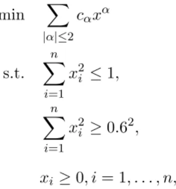
Example 3. Bi-quadratic POPs

(41)

specific bi-quadratic POPs, min x∈_Rn_,y_∈ Rm p0= X 1≤i<j≤n 1≤a<b≤m xixjyayb s.t. _kx_k2 = 1,_ky_k2 = 1, (1.30)

where k · k is the standard 2-norm in Euclidean spaces. It is clear that problem (1.30) is equivalent to min x∈Rn,y∈Rm p0 = 1 4[x T₍_e neTn−In)x][yT(emeTm−Im)y] s.t. _kx_k2= 1,_ky_k2 = 1,

whereen, em are all-one vectors of appropriate dimension andIn, Im are diagonal matrices of dimensionn×nandm×m. It is then easy to see the optimal value is−14(max{n, m}−1). By defining an index set

S(n) ={(i, j, k)∈N3 :i= 1, . . . , n−1, j =i+ 1, . . . , n, k= (n− i

2)(i−1) +j−i}

for additional variables, we can reformulate problem (1.30) as a quadratic problem by introducing additional variables,

min X 1≤k≤|S(n)| 1≤c≤|S(m)| wkzc s.t. wk =xixj,∀(i, j, k)∈S(n), zc=yayb,∀(a, b, c)∈S(m), kx_k2 = 1,_ky_k2= 1, (1.31)

wherew, z∈Rm with|S(n)|=n(n−1)/2,|S(m)|=m(m−1)/2. Letu=

x;y;w;z

(42)

a positive semedefinite relaxation can be applied to problem (1.31), min X n+m+1≤p≤n+m+|S(n)| n+m+|S(n)|+1≤q≤n+m+|S(n)|+|S(m)| Qpq s.t. un+m+k=Qij,∀(i, j, k)∈S(n), u_n₊_m₊|S(n)|+c=Qn+a,n+b,∀(a, b, c)∈S(m), n X i=1 Qii= 1, n+m X i=n+1 Qii= 1,    1 uT u Q   ∈ C ∗ n+m+|S(n)|+|S(m)|+1,2(Rn+m+ |S(n)|+|S(m)|+1₎_. (1.32)

Note that problem (1.32) is a simple SDP relaxation for problem (1.30). More elaborated SDP relaxations that provide bounds with guaranteed performance are discussed for this type of problem in [75].

Proposition 9. Problem (1.32) is unbounded.

Proof. Let ¯u be a (n+m+|S(n)|+|S(m)|)×1 all-zero vector and let ¯Q be a (n+m+

|S(n)|+|S(m)|)×(n+m+|S(n)|+|S(m)|) matrix such that

¯

Q11= ¯Qn+1,n+1= 1,Q¯n+m+1,n+m+1 = ¯Qn+m+|S(n)|+1,n+m+|S(n)|+1 =M2,

¯

Qn+m+1,n+m+|S(n)|+1 = ¯Qn+m+|S(n)|+1,n+m+1=−M,

whereM is a positive number and let all other entries for ¯Qbe 0. It is clear that (¯u,Q¯) is a feasible solution to problem (1.32). However, asM _{→ ∞}, the objective function goes to

−∞, thus the problem is unbounded.

(43)

bound. However, a CPSD tensor cone can be directly applied to problem (1.30), min hT4(p0), Xi s.t. _hT4(kxk2), Xi= 1, hT4(kyk2), Xi= 1, hT4(1), Xi= 1, X _{∈ C}_n∗₊_m₊₁_,₄(Rn+m+1). (1.33)

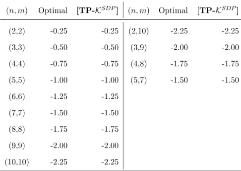
Problem[TP-_KSDP]can be used to approximate problem (1.33) and the results are listed in Table 1.5.2. In Table 1.5.2, we can see that relaxation [TP-_KSDP] can provide the optimal value for problem (1.32) while relaxation [QPSDP] for the QCQP reformulation of problem (1.32) fails to give a bound.

(n, m) Optimal [TP-_KSDP] (n, m) Optimal [TP-_KSDP] (2,2) -0.25 -0.25 (2,10) -2.25 -2.25 (3,3) -0.50 -0.50 (3,9) -2.00 -2.00 (4,4) -0.75 -0.75 (4,8) -1.75 -1.75 (5,5) -1.00 -1.00 (5,7) -1.50 -1.50 (6,6) -1.25 -1.25 (7,7) -1.50 -1.50 (8,8) -1.75 -1.75 (9,9) -2.00 -2.00 (10,10) -2.25 -2.25

Table 1.5.2: Relaxation comparisons for Example 3

(44)

Consider the following nonconvex QCQP, min f0(x) =−8x21−x1x2−13x22−6x1−x2 s.t. f1(x) =x21+x1x2+ 2x22−3x1−3x2−7≤0, f2(x) = 2x1x2+ 33x1+ 15x2−10≤0, f3(x) =x1+ 2x2−6≤0, x1, x2≥0 (1.34)

The optimal solution of the example isx∗_{= (0}_,₀_.₆₆₆₇₎T _with_f

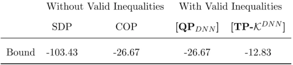
0(x∗) =−6.4444 (see [119]). A semidefinite relaxation and a copositive relaxation has been studied in [119], which gives a bound of -103.43 and -26.67 respectively for problem (1.34) (refer to Table 2 in [119], (SDP+RLT) is actually a DN N relaxation for copositive programming).

For tensor relaxations, we manually add valid inequalities to make the problem a 4-th degree POP, min f0(x) =−8x2₁−x1x2−13x2₂−6x1−x2 s.t. f1(x) =x21+x1x2+ 2x22−3x1−3x2−7≤0, f2(x) = 2x1x2+ 33x1+ 15x2−10≤0, f3(x) =x1+ 2x2−6≤0, x2f2(x)≤0, x2₁f1(x)≤0, x1, x2≥0 (1.35)

then[TP-KDN N_]_{can be used to approximate Problem (1.35), we obtain a bound of}₋₁₂_._83, which provides better bounds than SDP relaxation and completely positive relaxation on problem (1.34). We also add the valid inequalities x2f2(x) ≤ 0, x2₁f1(x) ≤ 0 directly to problem (1.34) by reformulating problem (1.35) as a quadratic program by adding additional variables and constraints as in (1.16):

(45)

min f0(x) =−8x21−x1x2−13x22−6x1−x2 s.t. ₋y1=x21+x1x2+ 2x22−3x1−3x2−7≤0, −y2= 2x1x2+ 33x1+ 15x2−10≤0, f3(x) =x1+ 2x2−6≤0, y3=x2₁, −x2y2 ≤0, −y1y3≤0, x1, x2, y1, y2, y3 ≥0.

In addition to adding valid inequalities to strengthen the tensor relaxation, adding positive semidefinite (PSD) reformulation linearization technique (RLT) constraints can further strengthen the relaxations. Similar to second order RLT introduced in [28], with the constraint hT4(1), Xi = 1 and conic constraint X ∈ C3∗,4(R3), for a quadratic constraint c0+c10x1+c01x2+c11x2₁+c12x1x2+c22x2₂ ≥0, following PSD-RLT constraints for CP tensor relaxation of problem (1.35) can be constructed,

(c0+c10x1+c01x2+c11x2₁+c12x1x2+c22x2₂)X(0,0,·,·)

=c0X(0,0,·,·)+c10X(1,0,·,·)+c01X(2,0,·,·)+c11X(1,1,·,·)+c12X(1,2,·,·)+c22X(2,2,·,·)0, (1.36)

whereX(0,0,·,·)0 as discussed in Section 1.5.1. Note that the PSD-RLT can’t be used in the CP relaxations on the QCQP reformulation. With the PSD-RLT constraints based on constraints, the optimal value is obtained at -6.4444. A comparison of bounds is listed in Table 1.5.3.

(46)

Without Valid Inequalities With Valid Inequalities SDP COP [QPDN N] [TP-KDN N]

Bound -103.43 -26.67 -26.67 -12.83

Example 5. Random Objective Function on a Feasible Region

In this example, we will present our preliminary numerical results on randomly gener-ated 4th degree POPs with feasible regions. The test problem is

min Randomly generated 4th degree homogenous polynomial of 3 variables s.t. (x1−0.5)2+ (x2−0.5)2+ (x3−0.5)2 ≥0.22,

(x1−0.5)2+ (x2−0.5)2+ (x3−0.5)2 ≤0.62, 0≤x1, x2, x3 ≤1,

(1.37)

The coefficients in the objective function are integers in the range [−5,5]. The first and second constraints make the problem nonconvex and it is easy to see the problem is feasible. We use [TP-KDN N_] _{to directly approximate problem (1.37) and} _[QP

DN N] to approximate the QCQP reformulation of problem (1.37). We denote ratioas the improve ratio similar to that in [119] and

ratio= [TP-K

DN N_] ₋_[QP

DN N]

fopt−[QPDN N]

.

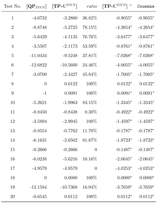
We also add PSD-RLT constraints for (x1−0.5)2 + (x2−0.5)2+ (x3−0.5)2 ≥ 0.22 and (x1−0.5)2+ (x2 −0.5)2+ (x3−0.5)2 ≤0.62 to problem (1.37). In Table 1.5.4, the relaxation [TP-_KDN N]with PSD-RLT constraints provides the tightest bounds where for instances optimal values are obtained. Relaxation [TP-_KDN N] provides tighter bounds than [QPDN N] for most test instances. For instances 8,9,18 and 20, relaxation

(47)

[TP-KDN N_] _{gives the optimal objective value, while} _[QP

DN N] is not tight. For instances 15 and 17,[TP-_KDN N]and[QPDN N]give the same bound. An average of 50% improve ratio implies that [TP-_KDN N] provides tighter bounds than [QPDN N] for Problem (1.37). In Table 1.5.4, relaxation [TP-_KDN N] provides tighter bounds than[QPDN N] for most test instances. For instances 8,9,18 and 20, relaxation[TP-_KDN N]gives the optimal objective value, while[QPDN N] is not tight. For instances 15 and 17, [TP-KDN N] and [QPDN N] give the same bound. An average of 50% improve ratio implies that [TP-KDN N_]_provides better relaxations than[QPDN N]for Example 5.

(48)

Test No. [QPDN N] [TP-KDN N] ratio [TP-KDN N] + Couenne 1 -4.6732 -3.2860 36.82% -0.9055∗ _-0.9055∗ 2 -8.8748 -5.2725 78.15% -4.2654∗ -4.2654∗ 3 -5.6429 -4.1135 76.76% -3.6477∗ -3.6477∗ 4 -3.5507 -2.1173 53.59% -0.8761∗ -0.8761∗ 5 -11.0434 -9.5248 37.81% -7.0268∗ -7.0268∗ 6 -12.6822 -10.5600 24.46% -4.0055∗ -4.0055∗ 7 -3.0709 -2.4427 45.84% -1.7005∗ _-1.7005∗ 8 0 0.0122 100% 0.0122∗ _0.0122∗ 9 -1 0.0091 100% 0.0091∗ _0.0091∗ 10 -5.2621 -1.9963 83.15% -1.3345∗ -1.3345∗ 11 -0.8450 -0.8438 0.30% -0.4922∗ -0.4922∗ 12 -3.5894 -2.9945 100% -1.4597∗ -1.4597∗ 13 -0.8554 -0.7762 11.70% -0.1787∗ -0.1787∗ 14 -6.1631 -2.6502 81.87% -1.8723∗ -1.8723∗ 15 -0.2666 -0.2666 0 -0.1487∗ -0.1487∗ 16 -6.0238 -5.6216 10.16% -2.0645∗ _-2.0645∗ 17 -4.9579 -4.9579 0 -4.0253∗ _-4.0253∗ 18 0 0.0080 100% 0.0080∗ _0.0080∗ 19 -12.1584 -10.7368 16.94% -3.7659∗ -3.7659∗ 20 -0.6545 0.0112 100% 0.0112∗ 0.0112∗

∗: Optimal value is obtained.

[TP-KDN N_]+_: _[TP-_KDN N_]_{with PSD-RLT constraints.}

Example 6. Numerical Results on Random Generated Polynomial Problems

(49)

polynomial optimization problems. The objective function is a 4th degree homogenous polynomial of 3 variables, with two 4th degree polynomial inequality constraints, a linear inequality constraint and nonnegative variables. The coefficients in the objective function are integers in the range [₋5,5] and the coefficients of the two polynomial constraints are integers in the range [₋10,10] and the coefficients of linear constraint are integers in the range [0,5], with a right hand side coefficient in the range [5,15]. We generated problems and send them to Couenne, for those problems which are feasible in Couenne, we use [TP-KDN N_]_{to directly approximate Example 6 and}_[QP

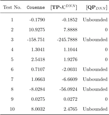
DN N]to approximate the QCQP reformulation of Example 6. Note that the convexity of these problems is not tested. Results are shown in Table 1.5.5, and we can clearly see that relaxation [QPDN N] fail to give a valid bound for instances 1,3,6,7,8 and 10, while tensor relaxation[TP-_KDN N] can provide a valid lower bound for all tested instances.

Test No. Couenne [TP-KDN N_] _[QP DN N] 1 -0.1790 -0.1852 Unbounded 2 10.9275 7.8888 0 3 -158.751 -245.7888 Unbounded 4 1.3041 1.1044 0 5 2.5418 1.9276 0 6 0.7107 -2.0031 Unbounded 7 1.0663 -6.6609 Unbounded 8 -8.0284 -56.0924 Unbounded 9 0.0275 0.0272 0 10 8.0032 2.4765 Unbounded

(50)

1.6 Conclusion

This chapter presents convex relaxations for general POPs over CP and CPSD tensor cones discussed in [64]. Bomze showed that completely positive matrix relaxation beats Lagrangian relaxations for quadratic programs with both linear and quadratic constraints in [18]. A natural question is whether similar results hold for general POPs that are not necessarily quadratic. Introducing CP and CPSD tensors to reformulate or relax general POPs, we generalize Bomze’s results in QPs to general POPs, that is, the CP tensor re-laxation beats Lagrangian rere-laxation bounds for general POPs with degree higher than 2. These results provide another way of using symmetric tensor cones to globally approxi-mate nonconvex POPs. Burer in [27] showed that every quadratic programs with linear constraints and binary variables can be reformulated as CP programs and programs with quadratic constraints can be relaxed by CP programs, with approximation approaches for CP matrix programs. Note that one can reformulate general POPs as QPs by introduc-ing additional variables and constraints and then apply Burer’s results to obtain global bounds on general POPs. Pena et al. generalize Burer’s results in [92] that under cer-tain conditions a general POP can be reformulated as a conic program over CP tensors. A natural question is which reformulations or relaxations will provides better bounds for general POPs. In this paper, we showed that the bound of CP tensor relaxations is better than the bound of CP matrix relaxations for the quadratic reformulation of some classes of general POP. This validates the advantages of using tensor cones for convexification of nonconvex POPs . We also provide some tractable approximations of the CP tensor cone as well as CPSD tensor cone, which allows the possibility to compute the bounds of these tensor relaxations. Some preliminary numerical results on small scale POPs showed that these tensor cone approximations can provide bounds for global optimum of the original POPs. More importantly, in the experiments, the bounds obtained by CP or CPSD tensor cone programs yield better bounds than the CP or SDP matrix relaxations for quadratic reformulation of general POPs with similar computational efforts.

(51)

As future work we plan to characterize the classes of POPs in which the CP and CPSD tensor cone relaxations provide better bounds than the CP and PSD matrix relaxations for quadratic reformulations of POPs. Also, more POP instances with larger sizes can be tested and numerical comparisons on these more complicated POP cases can be made by developing appropriate code to address these problems.

(52)

Chapter 2 Alternative LP and SOCP

Approaches for PO

2.1 Introduction

Many real-world problems can be modeled as a polynomial optimization problem (POP), thus devising new approaches to globally solve POPs is an active area of research [see, e.g., 5, 17, for recent surveys in this area]. In his seminal work, Lasserre [66] showed that semidefinite programming (SDP) [110] relaxations based on sum of square(SOS) polyno-mials [see, e.g., 17] can provide global bounds for POPs. However, the SDP constraints are computationally expensive and thus even using low-orders of the hierarchy to approx-imate large-scale POPs becomes computationally intractable in practice [69]. To improve the computational performance of the SDP based hierarchies to approximate the solution of POPs, prior work has focused on exploiting the problem’s sparsity [60] and symmetry [34, 42], improving the relaxation by generating and adding appropriate valid inequalities [46], using bounded SOS polynomials [70] and more recently by devising more compu-tationally efficient hierarchies such as linear programming (LP) and second-order cone programming (SOCP) hierarchies [2, 36, 37, 45, 91].

(53)

introduced by Ahmadi and Majumdar [2]. In particular, we show that SOCP hierarchies can be effectively used to strengthen hierarchies of LP relaxations for general POPs. Such hierarchies of LP relaxations have received little attention in the POP literature (a few noteworthy exceptions are [32, 36, 37, 68, 121]). However, in [61] we show that this solution approach is substantially more effective in finding solutions of certain POPs for which the more common hierarchies of SDP relaxations are known to perform poorly [see, e.g., 45]. Furthermore, when the feasible set of the POP is compact, these SOCP hierarchies converge to the POP’s optimal value. Note that for the well-known SDP based hierarchies introduced by Lasserre [66], thequadratic module(QM) [5] associated with the feasible set of the POP is required to be Archimedean [17], which implies the compactness of the POP’s feasible set.

The remainder of the chapter is organized as follows. We briefly review several convex approximations of POPs in Section 2.2. The proposed approximation strategies and hier-archies are presented in Section 2.3. Numerical results based on the proposed hierhier-archies are presented in Section 2.4. Section 2.5 provides some concluding remarks.

2.2 Preliminaries

The following notation is used throughout the chapter: let Rd[x] :=Rd[x1, . . . , xn] be the set of polynomials inn variables with real coefficients of degree at mostd. We define

SOS2d:= ( _k X i=1 pi(x)2:pi(x)∈Rd[x], k∈Z+ ) ,

as the cone of SOS polynomials in R2d[x] . For any S ⊆ Rn, let Pd(S) be the cone of polynomials in Rd[x] of degree at most d that are non-negative over the set S [see, e.g., 17]. We consider the following general POP,

(54)

min x f(x)

s.t. gi(x)≥0, i= 1, . . . , m,

x∈Rn,

(PP-P)

where the degree of the program is d = max_{deg(f),deg(g1), . . . ,deg(gm)}. Given S =

{x _∈ Rn : gi(x) ≥ 0, i = 1, . . . , m}, problem (PP-P) can be equivalently rewritten as the followingconic program [see, e.g., 23],

max

x,λ λ

s.t. f(x)₋λ_{∈ P}d(S),

x∈Rn, λ∈R.

(PP-D)

In general, solving (PP-P) is NP-hard [85]. Problem (PP-D) is a (linear) conic program whose complexity is captured in the cone_Pd(S), which is nottractable in general. Consid-ering a sequence of tractable cones Kr _{⊆ K}r+1 _{⊆ · · · ⊆ P}

d(S), then the following convex program max x,λ λ s.t. f(x)₋λ_{∈ K}r, x∈Rn, λ∈R (2.1)

provides a lower bound for (PP-D), and hence a lower bound for (PP-P). Above, by tractablewe mean that inclusion on the set can be expressed as alinear matrix inequalities (LMI) [5]. Asr increases in (2.1), a tighter bound is achieved. The choice of the tractable cone Kr _{is a key factor in obtaining good approximation bounds for (PP-D), and in turn} for (PP-P).

(55)

relax-ations to approximate Pd(S), where Kr = ( p(x)∈R2r[x] :p(x) =s0(x) + m X i=1

si(x)gi(x), s0(x)∈SOS2r, si(x)∈SOS2br−deg(gi)/2c )

,

(2.2)

and r _{≥ d}d/2_e is the level of the hierarchy. In this case, problem (2.1) is equivalent to

max x,si(x) λ s.t. f(x)₋λ=s0(x) + m X i=1 si(x)gi(x),

s0(x)∈SOS2r, si(x)∈SOS2br−deg(gi)/2c, i= 1, . . . , m,

λ∈R.

(QM-SOSr)

Problem (QM-SOSr) can be reformulated as a SDP [see, e.g., 17]. Under some condi-tions related to the compactness of the set S (more precisely, when the quadratic module generated by the set of polynomials {g1(x), . . . , gm(x)} is Archimedean), the hierarchy of problems (QM-SOSr) converges to the global solution of (PP-P) as r → ∞ [66]. How-ever, as r increases, the size of the positive semidefinite matrices required to reformulate (QM-SOSr) as a SDP increases exponentially. As a result, this approach is computation-ally expensive for large-scale problems [see, e.g., 44] or even for small-scale problems that require the solution of high levels of the hierarchy to obtain tight approximations of the POP of interest [see, e.g., 2, 46, 70].

Ahmadi and Majumdar [2] recently proposed a restriction of the SOS condition to ad-dress this shortcoming of the SDP-based hierarchies. The restriction of the SOS condition is done by introducing the use of diagonally dominant sum of square (DSOS) polynomi-als and scaled diagonally dominant sum of square (SDSOS) polynomials instead of SOS polynomials in (QM-SOSr).

(56)

for all i∈J, andαi, βij ∈R+ for alli, j∈J. Then p(x) =X i αimi(x)2+ X i,j βij(mi(x)±mj(x))2, (2.3)

is a DSOS polynomial in R2d[x]. Equivalently, DSOS polynomials can be defined as those that can be constructed from a diagonally dominant matrix (DD). Namely, let z(x) be a vector with the monomialsmi(x)for alli∈J, andQ∈R|J|×|J|be a (symmetric) diagonally dominant matrix. Then p(x) =zT(x)Qz(x) is a DSOS.

Let DSOS2d be the set of all DSOS polynomials in R2d[x]. Then it is clear from (2.3) thatDSOS2d⊆SOS2d. Thus, using DSOS polynomials instead of SOS polynomials in (QM-SOSr) provides a hierarchy of lower bounds for the SOS hierarchy. Moreover the resulting DSOS hierarchy is computationally easier to solve. Namely, recall that a symmetric matrixA∈Rn×n is DD ifAii≥P_j6=i|Aij|,∀i= 1, . . . , n. Thus the associated DSOS hierarchy max λ,di(x) λ s.t. f(x)₋λ=d0(x) + m X i=1 di(x)gi(x),

d0(x)∈DSOS2r, di(x)∈DSOS2br−deg(gi)/2c,

λ∈R,

(QM-DSOSr)

can be reformulated as a LP. As proposed by Ahmadi and Majumdar [2], the DSOS hi-erarchy (QM-DSOSr) can be strengthened by consideringscaled diagonally dominant sum of square (SDSOS) polynomials.

Definition 8 (SDSOS polynomials [2]). Let J be an index set, mi(x)∈Rd[x]be a mono-mial for all i_∈J, andαi, βi, βj ∈R+ for alli, j ∈J. Then

p(x) =X i αimi(x)2+ X i,j (βimi(x)±βjmj(x))2, (2.4)