Discriminant analysis based feature extraction for pattern recognition

(1)

DISCRIMINANT ANALYSIS BASED FEATURE

EXTRACTION FOR PATTERN RECOGNITION

W E I Wu

A THESIS IN

THE DEPARTMENT OF

ELECTRICAL AND COMPUTER ENGINEERING

PRESENTED IN PARTIAL FULFILLMENT OF THE REQUIREMENTS FOR THE DEGREE OF DOCTOR OF PHILOSOPHY

CONCORDIA UNIVERSITY MONTREAL, QUEBEC, CANADA

SEPTEMBER 2 0 0 9

(2)

**1*1**

Library and Archives Canada Published Heritage Branch Biblioth&que et Archives Canada Direction du Patrimoine de l'6dition 395 Wellington Street Ottawa ON K1A 0N4 Canada 395, rue Wellington Ottawa ON K1A0N4 Canada

Your file Votre reference ISBN: 978-0-494-63403-5 Our file Notre reference ISBN: 978-0-494-63403-5

NOTICE: AVIS:

The author has granted a

non-exclusive license allowing Library and Archives Canada to reproduce, publish, archive, preserve, conserve, communicate to the public by

telecommunication or on the Internet, loan, distribute and sell theses

worldwide, for commercial or non-commercial purposes, in microform, paper, electronic and/or any other formats.

L'auteur a accorde une licence non exclusive permettant a la Biblioth&que et Archives Canada de reproduire, publier, archiver, sauvegarder, conserver, transmettre au public par telecommunication ou par I'lnternet, preter, distribuer et vendre des theses partout dans le monde, a des fins commerciales ou autres, sur support microforme, papier, electronique et/ou autres formats.

The author retains copyright ownership and moral rights in this thesis. Neither the thesis nor substantial extracts from it may be printed or otherwise reproduced without the author's permission.

L'auteur conserve la propriete du droit d'auteur et des droits moraux qui protege cette these. Ni la these ni des extraits substantiels de celle-ci ne doivent etre imprimes ou autrement

reproduits sans son autorisation.

In compliance with the Canadian Privacy Act some supporting forms may have been removed from this thesis.

While these forms may be included in the document page count, their removal does not represent any loss of content from the thesis.

Conformement a la loi canadienne sur la protection de la vie privee, quelques formulaires secondaires ont ete enleves de cette these.

Bien que ces formulaires aient inclus dans la pagination, il n'y aura aucun contenu manquant.

(3)

(4)

ABSTRACT

Discriminant Analysis Based Feature Extraction for Pattern

Recognition

Wei Wu, Ph.D.

Concordia University, 2009

Fisher's linear discriminant analysis (FLDA) has been widely used in pattern recognition applications. However, this method cannot be applied for solving the pattern recognition problems if the within-class scatter matrix is singular, a condition that occurs when the number of the samples is small relative to the dimension of the samples. This problem is commonly known as the small sample size (SSS) problem and many of the FLDA variants proposed in the past to deal with this problem suffer from excessive computational load because of the high dimensionality of patterns or lose some useful discriminant information. This study is concerned with developing efficient techniques for discriminant analysis of patterns while at the same time overcoming the small sample size problem. With this objective in mind, the work of this research is divided into two parts.

In part 1, a technique by solving the problem of generalized singular value decomposition (GSVD) through eigen-decomposition is developed for linear discriminant analysis (LDA). The resulting algorithm referred to as modified GSVD-LDA (MGSVD-LDA) algorithm is thus devoid of the singularity problem of the scatter matrices of the traditional LDA methods. A theorem enunciating certain properties of the discriminant

(5)

subspace derived by the proposed GSVD-based algorithms is established. It is shown that if the samples of a dataset are linearly independent, then the samples belonging to different classes are linearly separable in the derived discriminant subspace; and thus, the proposed MGSVD-LDA algorithm effectively captures the class structure of datasets with linearly independent samples.

Inspired by the results of this theorem that essentially establishes a class separability of linearly independent samples in a specific discriminant subspace, in part 2, a new systematic framework for the pattern recognition of linearly independent samples is developed. Within this framework, a discriminant model, in which the samples of the individual classes of the dataset lie on parallel hyperplanes and project to single distinct points of a discriminant subspace of the underlying input space, is shown to exist. Based on this model, a number of algorithms that are devoid of the SSS problem are developed to obtain this discriminant subspace for datasets with linearly independent samples.

For the discriminant analysis of datasets for which the samples are not linearly independent, some of the linear algorithms developed in this thesis are also kernelized.

Extensive experiments are conducted throughout this investigation in order to demonstrate the validity and effectiveness of the ideas developed in this study. It is shown through simulation results that the linear and nonlinear algorithms for discriminant analysis developed in this thesis provide superior performance in terms of the recognition accuracy and computational complexity.

(6)

ACKNOWLEDGEMENTS

I would like to take this opportunity to express my deep gratitude to my supervisor, Professor M. Omair Ahmad, for his constant support, encouragement, patience, and invaluable guidance during this research. I am grateful to him for spending many hours with me in discussion about my research. The useful suggestions and comments provided by the members of the supervisory committee, Dr. M. N. S. Swamy, and Dr. Weiping Zhu, the committee member, external to the program, Dr. Terry Fancott, and the external examiner, Dr. Wu-Sheng Lu, as well as those of the anonymous reviewers of my journal papers are also greatly appreciated.

My sincere thanks go to my parents, family members, and relatives for their support and encouragement during my research. Special thanks to my husband, Weimin Zhu, whose patience, love, and unlimited support have made the successful completion of this thesis a reality. I would like also to mention my little son, Wuhua, whose beautiful face always refreshes my mind.

I am indebted to my friend, Mr. Jijun He, for fruitful discussions, suggestions and encouragement during the course of my doctoral study.

(7)

LIST OF FIGURES

Figure 2.1: Examples of (a) LS set of sample points and (b) NLS set of sample points ..10 Figure 4.1: The recognition accuracy and numerical errors of MGSVD-KDA with respect

to the order of the polynomial kernel function 79 Figure 4.2: The recognition accuracy and numerical errors of MGSVD-KDA with respect

to the parameter of the RBF function 80 Figure 5.1: Sample projections in a two-dimensional discriminant subspace using

algorithms (a) Algorithm A, (b) Algorithm B, (c) Algorithm C and (d)

Algorithm KC 105 Figure 5.2: Sample projections in a two-dimensional discriminant subspace using

algorithms (a) MGSVD-LDA and (b) MGSVD-KDA 106 Figure 5.3: Sample projections in a two-dimensional discriminant subspace using

algorithms (a) RLDA and (b) KRDA 106 Figure 5.4: Sample projections in a two-dimensional discriminant subspace using

algorithms (a) PCA+LDA and (b) KPCA+LDA 107 Figure B.l: Images of one subject in the FERET face database 135 Figure B.2: Images of one subject in the YALE face database 136 Figure B.3: Images of one subject in the AR face database 136 Figure B.4: Images of one subject in the ORL face database 137

(11)

LIST OF TABLES

Table 3.1: MGSVD-LDA algorithm 37

Table 3.2: M G S V D - K D A algorithm 42

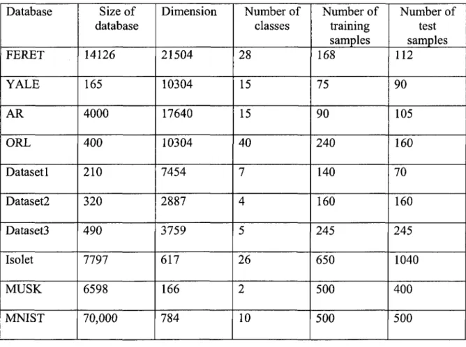
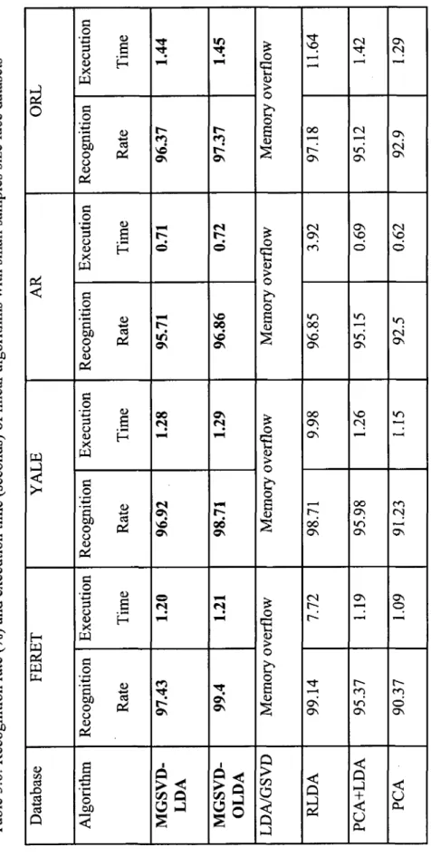
Table 3.3: MGSVD-OLDA algorithm 45 Table 3.4: MGSVD-OKDA algorithm 47 Table 3.5: Summary of databases 53 Table 3.6: Recognition rate (%) and execution time (seconds) of linear algorithms with

small samples size face datasets 54 Table 3.7: Recognition rate (%) and execution time (seconds) of linear algorithms with

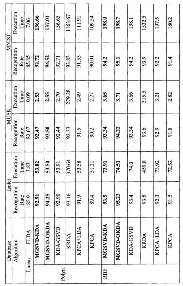
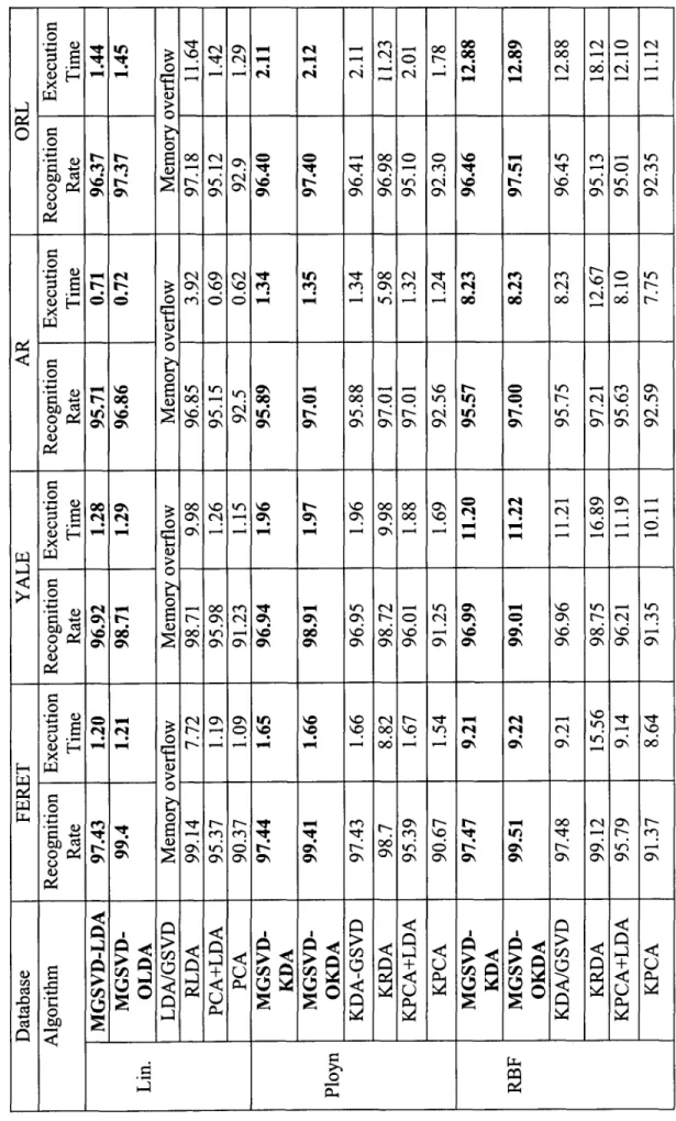
small samples size text document datasets 55 Table 3.8: Recognition rate (%) and execution time (seconds) of kernelized algorithms

with large samples size datasets 58 Table 4.1: Recognition rate (%) and execution time (seconds) of kernelized algorithms

with small samples size face datasets 75 Table 4.2: Recognition rate (%) and execution time (seconds) of kernelized algorithms

with small samples size text document datasets 76 Table 4.3: The maximum differences between the theoretical values and computed values

of the inter- and intra-class distances in the discriminant subspace derived

from the MGSVD-LDA algorithm using face databases * 78 Table 4.4: The maximum differences between the theoretical values and computed values

of the inter- and intra-class distances in the discriminant subspace derived

from the MGSVD-LDA algorithm using text document databases * 79

Table 5.1: Algorithm A 92 Table 5.2: Algorithm B 94

(12)

Table 5.3: Algorithm C 96 Table 5.4: Algorithm KC 100 Table 5.5: Performance of the three proposed linear algorithms 108

Table 5.6: Recognition rate (%) and execution time (seconds) of the proposed and some

other linear algorithms with small sample size databases I l l Table 5.7: Recognition rate (%) and execution time (seconds) of the proposed and some

(13)

LIST OF ABBREVIATIONS

SSS: Small sample size

LDA: Linear discriminant analysis

FLDA: Fisher's linear discriminant analysis RLDA: Regularized linear discriminant analysis PCA: Principal component analysis

SVD: Singular value decomposition

GSVD: Generalized singular value decomposition

MGSVD: Modified generalized singular value decomposition KDA: Kernelized discriminant analysis

KPCA: Kernelized principal component analysis KFD: Kernel Fisher discriminant

GDA: Generalized kernel discriminant analysis DS: Discriminant subspace

LS: Linearly separable NLS: Nonlinearly separable PR: Pattern recognition

(14)

LIST OF ACRONYMS

AW: Within-class scatter matrix of linearly independent samples

AB: Between-class scatter matrix of linearly independent samples

Ac: Total scatter matrix of linearly independent samples

X : Input matrix consists of m-dimensional samples x(>.

m: Dimensionality of samples

n: Number of input samples N: Number of classes

i: Class number

ni: Number of samples of zth class

x,: Sample vector

\tj: jih sample in z'th class,

c : Global centroid vector

c( , ): Centroid vector of the z'th class

S,: Total scatter matrix

Sw: Within-class scatter matrix

SA: Between-class scatter matrix

: Eigenvalues g;.: Eigenvectors

G: Transformation matrix

: m-dimensional input sample space r : Kernel feature space

K : Kernel matrix

(15)

ij/,: Mapped sample in kernel feature space

i|iy : jth mapped sample of z'th class in kernel feature space

»|/: Global centroid of mapped samples in feature space v|/(,): Centroid vector of z'th mapped class

Sw: Within-class scatter matrix in kernel feature space

Sb: Between-class scatter matrix in kernel feature space

S;: Total scatter matrix in kernel feature space

G : Transformation matrix in kernel feature space R( ): Range of associated matrix

N(-) : Null space of associated matrix (•) : Inner product of two vectors

(16)

Chapter 1 Introduction

1.1 Background

Pattern recognition is the discipline that studies how a machine can observe the environment, learn to distinguish patterns (samples), and make reasonable decisions on the classes of new patterns [1]. Pattern is a quantitative or structural description of an object or some other entity of interest. Depending on the applications, patterns can be handwritten cursive words, speech signals, odor signals, fingerprint images, animal footprints, human faces or any type of measurements that need to be classified.

One of the widely used pattern recognition approaches is the statistical pattern recognition. In the statistical approach, each pattern is represented in terms of m features. Depending on the measurements of an object, features in a pattern can be either discrete numbers or real continuous values. The requirement on features is that the features can reflect the characteristics of desired objects and differ from those other objects to the largest extent. For example, a face image, being a d x d array of 8 bit intensity values, can be represented as a vector of dimension m - d2. Thus, each pattern can be viewed as

an m-dimensional feature vector or a point in an m-dimensional space, that is, x = [X[, x2, • • •, xm ]

(17)

where x],x2,---,xm are the features. This space is called sample feature, feature space or

input space. For example, an image of size 256x256 becomes a 65536-dimensional

vector or equivalently, a point in a 65536-dimensional space.

The procedure of a statistical pattern recognition system has two main steps: training (learning) and classification (testing). In the training step, feature extraction creates a set of representative features based on transformations or combinations of the given patterns. The set of representative features is considered to be the most important and effective attributes in distinguishing the patterns from different classes. The classification step is to assign a class label to each new pattern.

Patterns, being similar in overall configuration, are not randomly distributed in the input space and thus can be described by a relatively low-dimensional subspace. The idea is to find appropriate features for representing the samples with enhanced discriminatory power for the purpose of recognition. This process is known as feature extraction. A commonly used feature extraction technique is to transform the original sample space into a lower-dimensional discriminant subspace, in which a transformed sample of the dataset is easily distinguished. The objective is to find a set of transformation vectors spanning over the discriminant subspace, on which the projections of the samples within each class condense into a compact and separated region.

1.2 Motivation

Two classical linear feature extractors are principal component analysis (PCA) [2] -[3], [7] - [8] and Fisher's linear discriminant analysis (FLDA) [4], [5], [6]. Both these methods extract features by projecting the original sample vectors onto a new feature

(18)

space through a linear transformation matrix. However, the goal of optimizing the transformation matrix in the two methods is different. In PCA, the transformation matrix is optimized by finding the largest variations in the original feature space [2] [3], [7] -[8], On the other hand, in FLDA, the ratio of the between-class and within-class variations is maximized by projecting the original features to a subspace [4], [5], [6], PCA is effective in restructuring the dataset, but it is weak in providing the class structure. FLDA formulates the class boundaries by finding a discriminant subspace in which different classes occupy compact and disjoint regions using the Fisher criterion

[5], [6]

_ | GrS „ G |

G ^ a r g m a x ^ - ^

where SB and Sw are, respectively, the between-class and within-class scatter matrices,

G is the transformation matrix whose columns are the projection vectors that span the discriminant subspace, and |*| denotes the determinant of the associated matrix. The solution to this maximization problem is the set of eigenvectors corresponding to the non-zero eigenvalues of the matrix S~'SA.

The Fisher linear discriminant analysis cannot be applied to solve pattern recognition problems if the within-class scatter matrix is singular, a situation that occurs when the number of the samples is small relative to the dimension of the samples. This is so-called the small sample size (SSS) problem [4]. Small sample size data with high dimensionality are often encountered in real applications, such as in human face recognition. Many FLDA variants have been proposed to address this singularity issue [9] - [46]. Tian et al.

(19)

et al. [16] have proposed a rank decomposition method based on successive eigen-decomposition of the total scatter matrix S, and the between-class scatter matrix SB. However, the above methods are typically computationally expensive since the scatter matrices are very large [17]. In [18], a two-stage FLDA method has been introduced, in which a principal component analysis is carried out for dimension reduction prior to applying the Fisher criterion. However, this dimension reduction step eliminates some useful discriminant information, since some of the eigenvectors of the total scatter matrix are discarded in order to make Sw non-singular [19] - [24]. In the direct LDA (D-LDA)

method [19], the null space of SA is first removed, and then the discriminant vectors in the

range of S6 are found by simultaneously diagonalizing SB and Sw [4], A drawback of this

method is that some significant discriminant information in the null space of Sw gets

eliminated due to the removal of the null space of SA [20], [22] - [24], In the regularized

FLDA (RLDA) [21], [29] - [33], the singularity problem is solved by adding a perturbation to the scatter matrix. The optimal perturbation parameter is normally estimated adaptively from the training samples through cross-validation, a process which is very time consuming. Some FLDA variants have attempted to overcome the SSS problem by using the generalized singular value decomposition (LDA/GSVD) [34], [35], However, these methods suffer from excessive computational load because of the large dimension of the samples [36]. Chen et al. [41] proposed the null space method based on the modified FLDA criterion

_ | GTSBG |

(20)

where S, is the total scatter matrix [42], [43]. However, the authors did not give an efficient algorithm for applying this method to solve the singularity problem of the Fisher criterion [47].

Since the linear feature extraction methods cannot capture the nonlinear class boundaries, which exist in many patterns and affect the recognition accuracy of the patterns, kernel machines [49] - [56] are used to map the patterns into a high-dimensional kernel feature space where the patterns are linearly separable, and thus, the linear feature extraction techniques can be applied in the mapped space. The integration of the kernel machine with a linear discriminant method provides a nonlinear algorithm with improved recognition accuracy [57] - [77]. However, nonlinear algorithms also suffer from the same problems as that inherent in the corresponding linear versions. Hence, the choice of a good linear algorithm is crucial to obtaining an efficient kernelized algorithm.

From the foregoing discussion, it is clear that the existing discriminant analysis techniques, in general, suffer from the excessive computational load in dealing with the high dimensionality of patterns or lose some useful discriminant information in order to overcome the singularity problem associated with the Fisher criterion. It is, therefore, necessary to conduct an in-depth study of the mechanism of the discriminant analysis leading to designs of efficient low computational complexity algorithms for feature extraction without having to deal with the SSS problem.

1.3 Scope of the Thesis

(21)

are devoid of the small sample size problem. With this unifying theme, the work of this study is carried out in two parts.

In part 1, a low-complexity algorithm that overcomes the singularity problem of the scatter matrices of the traditional FLDA methods is developed for linear discriminant analysis (LDA) by solving the problem of generalized singular value decomposition (GSVD) through eigen-decomposition. A theorem providing the distance between samples in the discriminant subspace derived from this GSVD-based algorithm is established to address the class structure and separability of linearly independent samples.

In part 2, a new systematic framework for the feature extraction of datasets with linearly independent samples is developed. Within this framework, a discriminant model is first established. It is shown that if the samples of a dataset are linearly independent, then the samples of the individual classes of the dataset lie on parallel hyperplanes and the samples of the entire class can be projected onto a unique point of a discriminant subspace of the underlying input space. A number of algorithms that are devoid of the SSS problem are developed to determine the discriminant subspace for datasets with linearly independent samples.

1.4 Organization of the Thesis

The thesis is organized as follows.

In Chapter 2, a brief review of the linear and nonlinear techniques for feature extraction is presented. This review is intended to facilitate the understanding of the development of the techniques for feature extraction presented in the thesis. This chapter

(22)

also includes some preliminaries on the commonly used techniques for dealing with the singularity problem associated with the Fisher criterion.

In Chapter 3, a new technique [37], referred to as the MGSVD-LDA algorithm that can effectively deal with the SSS problem, is presented by applying eigen-decomposition to solve the problem of the generalized singular value decomposition. A scheme is developed to kernelize the proposed linear algorithm to deal with the discriminant analysis of datasets in which samples are not linearly separable and a direct application of a linear algorithm fails to separate the classes of the datasets. In order to improve the recognition accuracy of the proposed linear and nonlinear algorithms further, a method is devised to take care of the over-fitting problem by orthogonalizing the basis of the discriminative subspace [38], [39]. Extensive simulation results are also presented in this chapter to demonstrate the effectiveness of the proposed linear, kernelized and orthogonalized algorithms and compare their performance with that of other existing algorithms.

In Chapter 4, a theorem that establishes the class structure and separability of linearly independent samples in the discriminant subspace derived from the proposed MGSVD-LDA algorithm is developed. This theorem is then used to develop a method to estimate the numerical errors of the proposed algorithms and also to control the kernel parameters to maximize the recognition accuracy of the kernelized algorithm.

In Chapter 5, a systematic framework for the pattern recognition of datasets with linearly independent samples is developed [40], A discriminant model, in which the samples of the individual classes of a dataset lie on parallel hyperplanes and project to single distinct points of the discriminant subspace of the underlying input space, is shown

(23)

to exist. In conformity with this model, three new algorithms are developed to obtain the discriminant subspace for datasets with linearly independent samples. A kernelized algorithm is also developed for the discriminant analysis of datasets for which the samples are not linearly independent. Simulation results are also provided in this chapter to examine the validity of the proposed discriminant model and to demonstrate the effectiveness of the linear and nonlinear algorithms designed based on the proposed model.

Finally, in Chapter 6, concluding remarks highlighting the contributions of the thesis and suggestions for some further investigation of the topics related to the work of this thesis are provided.

(24)

Chapter 2 Literature Review

2.1 Introduction

Feature extraction is one of the central and critical issues to solving pattern recognition problems. It is the process of generating a representative set of data from the measurements of an object, which are considered to be the most important and effective descriptors or characteristic attributes in distinguishing the object to belong to one class from another class. The main objective here is to find techniques that can introduce low-dimensional feature representation of objects, i.e., reduce the amount of data needed in representing objects, while achieving the best discriminatory power.

Feature extraction techniques, in general, can be classified into two categories: linear and nonlinear methods [1], [4], Linear methods can be applied when the samples are linearly separable. Two subsets U and V of are said to be linearly separable (LS) if there exists a hyperplane P in 5?m such that the samples of U and those of V lie on its

opposite sides. On the contrary, if they are nonlinearly separable (NLS), then a single hyperplane cannot be used to classify them [84], [87]. Figure 2.1 shows an example of LS and NLS set of sample points. In some cases, linear methods may not provide a sufficient discriminating power for nonlinearly separable samples. Nonlinear techniques, such as

(25)

kernel methods [49] - [56], can be used to transform the input samples into a higher dimensional kernel feature space by a nonlinear kernel mapping where samples become linearly separable so that the linear discriminant analysis can be applied in that high dimensional kernel feature space.

•

i—| ^ i n n

D #

•

(a) (b)

Figure 2.1: Examples of (a) LS set of sample points and (b) NLS set of sample points In this chapter, the linear feature extractors — principle component analysis (PCA) [2], [3], [7], [8], Fisher's linear discriminant analysis (FLDA) [5], [6] and some of the representative FLDA variants — are reviewed. Techniques to deal with the singularity problem of the scatter matrices of the traditional FLDA are explained in detail. Some nonlinear discriminant methods that can effectively deal with nonlinearly distributed patterns are also briefly discussed.

2.2 Linear Feature Extraction Techniques

Many linear methods have been proposed for feature extraction during the last two decades [2], [3], [5] - [46]. Among these methods, PCA and FLDA are the two most well-known and frequently used techniques. In PCA, the projection axes, along which the

(26)

variance of the projected components of all the sample vectors is maximized, are found. In FLDA, the optimal directions to project input samples in high-dimensional space onto a lower-dimensional space are searched with an objective of finding a discriminant subspace where different class categories occupy compact and disjoint regions.

2.2.1 Principle Component Analysis

Given a set of w-dimensional samples, the total covariance matrix can be formed as

where x, is the /th sample vector, n the sample size, and c the global centroid given by

c = - 5 > , (2-2)

n ,=\

PCA finds the set of projection directions, G ^ , in the sample space that maximize the total scatter across all the samples:

where G is the transformation matrix, GPCA is the optimal transformation matrix whose

columns are the orthonormal projection (transformation) vectors that can maximize the total scatter, and |*| denotes the determinant of the associated matrix. Essentially, this is an eigenvalue problem. If the eigenvectors are sorted in the order of descending eigenvalues, the variance of the projected samples along any eigenvector is larger than that along the next eigenvector in the sorted sequence. When the number of non-zero

7 _(2.1)

(27)

eigenvalues is less than the dimension of the original sample space, PCA can be used to project the samples from the original high-dimensional sample space to a subspace of the sample space to reduce the dimensionality of the samples and to set them as apart as possible.

Generally, if the original sample space is low-dimensional, the eigenvectors and eigenvalues of the matrix S, can be calculated directly. However, for a problem, such as face recognition using holistic whole-image based approach, the dimensionality of a face sample vector is always very high. A direct calculation of the eigenvectors of S; is

computationally expensive, or even infeasible on computers with low cache memory. The Eigenface technique [25] that determines the required eigenvectors has been proposed to deal with this problem. These eigenvectors are also called eigenfaces. In this method, S, is first expressed as

X T whereH, =—t=[X, -c,...,xn - c ] , and then an nxn matrix R = H , H , i s formed. In case

yjn

that the number of samples n is much smaller than the dimension m of the samples, the size of R is much smaller than that of S,, and hence, it is much easier to obtain its eigenvectors. Let u,, u2, ..., un_, be the orthonormal eigenvectors of R, corresponding to the n-1 largest eigenvalues \ > A2 >... > An_t . Then, the corresponding orthonormal eigenvectors of Sr are given by

Sl= - 2 ( X / - c X x , - c )r= H , H f n

,=,

1 (2.4) 1 (2.5)

(28)

The projection of the sample x, on the eigenvector g. is given by

T

yj=gj * = (2.6)

The resulting features, yv y2, ..., yn_,, form a PCA-transformed feature vector

y/ = b p y2> •••> y»-if for the samples x,, / = 1, ..., n.

2.2.2 Fisher's Linear Discriminant Analysis and its Variants

Fisher's Linear Discriminant analysis is one of the most prevalent linear feature extraction techniques for discriminant analysis. Similar to PCA, in FLDA, the optimal directions are obtained to project input high-dimensional samples onto a lower-dimensional subspace. However, while the key idea behind PCA is to find the directions along which the data variance is the largest, that behind FLDA is to search for the projection directions that simultaneously maximize the distance between the samples of different classes and minimize the distance between the samples of the same class. The class separability in low-dimensional representation is maximized in the FLDA method while it is not in PCA [1], [4]. FLDA-based algorithms usually outperform PCA-based ones because of the more rational objective and optimality criterion of the former.

Given a set of w-dimensional samples that consisting of N classes with the /th class having nt samples, the global centroid is given by (2.2) and the centroid of /th class is given by

(29)

(2.8)

where ki=nx+n2-\- ... + ni, and x, is the /th ( I = 1, 2, . . . , « ) sample vector, n the

N

sample size, « = , and i the class number, i - 1, ..., N. By using the three matrices, M

HI 5 Hw and H,, given by

H6 = [V^(c( 1 ) - c),..., - c)]

H;= - U (X l- c ) , . . . , ( xn- c ) ]

V"

the between-class and within-class and total scatter matrices can be defined as

S „ = H X . St = H X > S(= H , H( r (2.9)

respectively. The linear discriminant analysis employs the Fisher criterion given by

IGTS GI

Gflda =argmax * = [ g „ g2, ..., g j (2.10)

where G is the transformation matrix and GFLDA is the optimal transformation matrix

whose columns, g;, i = l ,2, ..., d, are the set of generalized eigenvectors of SA with

regard to Sw[5] corresponding to the d < N-\ largest generalized eigenvalues that is,

(30)

When the inverse of Swdoes exist, the generalized eigenvectors can be obtained by the

eigen-decomposition of S~'S6 . The new feature vectors y, are defined by Yi = GT x,, 1 = 1, 2, ..., n.

Through the above process of FLDA, the set of the transformation vectors is found to map the high-dimensional samples onto a low-dimensional space, the discriminant subspace, and at the same time, all the samples projected along this set of transformation vectors have the maximum between-class and minimum within-class scatters simultaneously.

It is seen that the Fisher linear discriminant analysis has a limitation in that it requires the within-class scatter matrix Sivto be non-singular, which is not the case in practice

when the SSS problem occurs, i.e., when the number of the samples is smaller than the dimension of the samples. Small sample size datasets with high dimensionality widely exist in real applications such as human face recognition and analysis of micro-array data. To deal with this limitation of the FLDA technique, a number of variants to this technique have been proposed in the literature.

1) PCA + FLDA Method

Swets and Weng [18] have proposed the PCA + FLDA method, also known as the Fisherface method, in order to solve the singularity problem of the Fisher criterion. In this method, in order to make Sw nonsingular, PCA is first applied to reduce the sample

(31)

representation of the samples and the transformation matrix G FLDA . The overall

transformation matrix of the PCA + FLDA method is given by

Gp, PCA+FLDA (2.12)

where GPCA can be obtained from (2.3), which rewritten here as

GPCA = argmax | GfS,G, | _O (2.13)

and GFWA is given by

GFLDA = a r g n (2.14)

with G, and G2 being the matrices whose columns are the projection vectors in the PCA

and FLDA transformed spaces, respectively, and Sj = G ^ S ^ G ^ and Sw = GTPCASWGPCA

A problem with this algorithm is that the discarded eigenvectors in its PCA part may contain some discriminant information, very useful to the FLDA part. Later, Chen et al. [41] have proved that the null space of Sw, as a matter of fact, contains the most

discriminative information. To avoid the loss of significant discriminant information due to the PCA preprocessing step, an algorithm, referred to as direct LDA (D-LDA), without a separate PCA step, has been proposed in [19].

2) Direct LDA (D-LDA) Method

In the D-LDA method [19], the idea of "simultaneous diagonalization" [4], [78] of SA

and Slv is employed to deal with the SSS problem. The matrix SB is first diagonalized and

(32)

The eigenvector matrix V that diagonalizes S6 is obtained by using

eigen-decomposition of S6 such that

VTSB\ = A (2.15)

where V is the eigenvector matrix and A is the eigenvalue matrix of SB. By keeping only the non-zero eigenvalues of A , (2.15) is re-written as

VrS4V = A6 (2.16)

where in this equation, the diagonal elements of AB, with the non-zero eigenvalues only, are arranged in a non-increasing order and V is the eigenvector matrix with the eigenvectors corresponding to the non-zero eigenvalues only. Next, using the matrix

Z = V A ^ (2.17) the S4 is diagonalized as

ZrS6Z = I (2.18)

and the matrix ZrSwZ is diagonalized using eigen-decomposition as

Ur( ZrSwZ ) U = Dw (2.19)

where U is the eigenvector matrix and Dw is the eigenvalue matrix of ZTSWZ. Finally, the transformation matrix is given by

(33)

In this algorithm, the null space of SB, which the authors of [19] claim to contain no useful information for discrimination, is ignored in the first step. However, Gao et al. [28] have pointed out that the D-LDA algorithm has a shortcoming in that ignoring of the null space of for dimension reduction would also neglect part of the null space of Sivand

would thus result in the loss of some useful discriminant information contained in the null space of Sw.

3) Regularized LDA Method

To deal with the singularity problem of the Fisher criterion, a regularized FLDA (RLDA) has been introduced in [29], [29]. The basic idea of the regularization technique is to add a constant a > 0 , known as the regularization parameter, to the diagonal elements of the scatter matrices. This parameter is estimated via cross-validation.

The way to deal with the singularity of scatter matrix Sw in the classical or S, in the

modified Fisher criterion [42] is to apply regularization by adding a constant to the diagonal elements of Sw or S,, i.e., Sw = Sw +al or S, = S, + al, where I is the identity

matrix of size m x m .

The classical Fisher criterion giving GFLDA is defined by (2.10), and the modified

Fisher linear discriminant criterion [4] is given by

GMFLDA = arg max (2.21)

° I Lr I where

(34)

S , = Sw + St (2.22)

Since Sw and S( are positive semi-definite, Sw and S, are also positive definite, and

hence, nonsingular. Then, the transformation matrix for the RLDA method, GRLDM or

GRLDA2 , can be obtained by using the following optimality criteria:

G , ^ =a r g n , a x | GJ( G s^G | (2.24)

The solution to (2.23) or (2.24) can be obtained by computing the eigen-decomposition of

(Sw + a I ) -!S4 or (S, +al)~x S4.

This method has a high computational load when the samples have a large dimension. Also, an adaptive estimation of the optimal regularization parameter from the training samples using cross-validation is very time-consuming. To overcome the shortcomings of the RLDA method, a number of improved RLDA algorithms have been proposed in the literature [21], [31]-[33],

4) Null Space Method

In order to overcome the singularity problem of the Fisher criterion, Chen et al. [41] have proposed the null space method based on the modified criterion [4] for Fisher's linear discriminant analysis.

(35)

projected onto the null space of Sw. The projection vectors thus obtained are finally

transformed into the projection vectors by applying PCA.

The algorithm given in [41] for applying the null space method in the original sample space is not efficient. A pixel grouping method is applied to extract geometric features so as to reduce the dimension of the sample space. It has been pointed out that the performance of this method depends on the dimension of the null space of Sw in the

sense that a larger dimension provides a better performance. Thus, a preprocessing step to reduce the original sample dimension should be avoided [47], [88], [89].

2.3 Nonlinear Feature Extraction Techniques

Although the linear discriminant methods described in the previous section are successful when the samples in datasets are linearly separable, they do not provide good performance when the samples do not follow such a pattern, since it is difficult to capture a nonlinear distribution of samples with linear mapping. As the distributions of most patterns in real world are nonlinear and very complicated, problem of pattern recognition of nonlinearly separable samples should be addressed using nonlinear methods. Kernel machine techniques [49] - [56] are a category of such nonlinear methods. The main idea behind these techniques is to transform the input space into a higher dimensional feature space by using a nonlinear kernel mapping where patterns become linearly separable so that the principles of linear discriminant analysis can be applied in the kernel feature space. The kernel functions allow such nonlinear extensions without explicitly forming a

(36)

nonlinear mapping, as long as the problem formulation involves the inner products between the mapped data points.

A kernel is a nonlinear mapping ® , designed to map the samples of the input space y{m into a higher-dimensional feature space T :

<X> . 9 T - > r

Correspondingly, the samples x, 's in the original input space are mapped into the kernel feature space T , where the classes of the resulting higher dimensional feature vectors 's become linearly separable. However, the high dimensionality of the feature space makes the feature extraction computationally infeasible. This problem is overcome by using the so-called "kernel trick" [54], in which the inner product of the mapped vectors in the feature space can be implicitly derived from the inner products between the input samples, such that

where (•) denotes the inner product of the two associated vectors, &(•) denotes a kernel function, and klh is a scalar. The key to a successful kernelization of a linear algorithm is in its ability to construct inner products in the input space and then to reformulate these products in the feature space. A number of kernelized discriminant analysis algorithms have been proposed with enhanced recognition accuracy [57] - [77]. In the next two subsections, the method of kernelizing linear algorithms is demonstrated using the linear principle component analysis [2] and Fisher's discriminant analysis [4] methods.

(37)

2.3.1 Kernelization of the Principle Component Analysis Method

The basic idea of the kernelized principle component analysis (KPCA) [57] is to map the input data into a new feature space T where the samples become linearly separable so that the linear PCA can be performed in that feature space.

Given a set of m-dimensional training samples x,, / = 1, 2, ..., n , the matrices and O are defined as

- V ) ] (2-26)

yjn

0 = [M/„M/2,...,Y|/„] (2.27)

where is the mapped sample vector corresponding to sample vector x, and \j/ is the global centroid of the mapped sample vectors in the kernel feature space.

Similar to the definition of the total scatter matrix S, in the input sample space, by using the matrix the total scatter matrix S, in the feature space is given as

S, = (2.28) The elements of the matrix R = <DrO are then determined by using the "kernel trick":

) = *((*/>**» (2-29) The mapped samples are centered around the global centroid by replacing the matrix R

by

(38)

where the matrix 1„ = (1 / n)nxn.

The orthonormal eigenvectors u,,u2,...,un_1 of R , corresponding to the n-1 largest

decomposition of R and the corresponding orthonormal eigenvectors of S, , gi> £2> •••> g„-i5 given by

form the kernelized transformation matrix.

2.3.2 Kernelization of the Fisher Linear Discriminant Analysis Method

FLDA is designed for linear pattern recognition applications. However, it fails to perform well for the recognition of patterns that are not linearly separable. To deal with this problem, nonlinear versions of FLDA have been proposed. First, Mika [58] formulated a kernelized Fisher discriminant (KFD) analysis method for a two-class case, and then Baudat [59] proposed a generalized kernel discriminant analysis (GDA) for datasets with multiple classes.

In basic idea of the GDA method is to first perform the centering in the kernel feature space by shifting each mapped sample vector using the global centroid, and then to apply the discriminant analysis in the centralized kernel feature space. In this method, given a non-zero eigenvalues,

X

x

>X

1

> ... >

A can be obtained by using the

(39)

set of m-dimensional training samples x/5 / = 1, 2, ..., n, consisting of N classes where

N

the /'th class has samples(thus, n = ^ ), first the following three matrices are defined: 1=1

y/n

yjn

(2.32)

where \|/, is the mapped sample vector corresponding to the input sample vector x,, \(/ (0 is the centroid of the mapped samples of the /th class, and v|/ is the global centroid of the mapped samples in the kernel feature space. The Fisher criterion can then be expressed as

G K - arg max GSBG

G S,„G (2.33)

where Sb and Sw are, respectively, the between-class and within-class scatter matrices

defined in the kernel feature space T as

(2.34)

S = ® & _{W WW} (2.35)

and G = [gA:i, gK2> • ••> gKdf 's the transformation matrix. The matrix G^is the optimal

(40)

largest eigenvalues obtained by solving the generalized eigenvalue problem: Sftgjcf = Ki • This generalized eigenvalue problem cannot be solved due to the high

dimensionality of the mapped sample vectors. This problem is solved by formulating an alternate generalized eigenvalue problem.

Let a(. = (an,...,ain)T, i = 1, 2, ..., d, such that

n

g , = X a „ V , = ® a , (2-36) /=i

where <J> is defined by (2.27). The transformation matrix G can be expressed as

G = O [ a „ a2, . . . , a J = <D0 (2.37)

where 0 = [ a1, a2, . . . , ar f] . Substituting (2.37) into (2.33), the Fisher criterion can be

expressed as [57]

0r( R W R ) 0

0 ^ = a r g m a x — (2.38) 0 _{0 ( R R ) 0}

where the matrix R is given by (2.30) and W = diag(W,,...W,.,...,Ww) is an nxn

block diagonal matrix with W( being an nt x nj diagonal matrix with all its diagonal elements equal to 1 / ni.

Conducting an eigen-decomposition of the matrix R yields

(41)

where P is the eigenvector matrix of R with PRP = I , and A is the eigenvalue matrix

with non-zero eigenvalues as its diagonal elements. Substituting (2.39) into (2.38), (2.38) can be expressed as 0K = arg max ( A2PR0 )R( A2PRW P A2) ( A2PR0 ) ( A2PR0 )RA ( A2PR0 ) (2.40) By letting B = A2P 0 (2.41)

Eqn. (2.40) can be expressed as

B a = arg max

B SAB BRS B

(2.42)

where Sb = A P WPA is semi-positive definite and Siv = A is positive definite. The

columns of the optimal transformed coefficient matrix B^, =[P,, P2, ..., P^]are actually

the eigenvectors of Sw Sb corresponding to the d (d < N -1) largest eigenvalues, and can

be obtained by eigen-decomposition of SwSb. Once the optimal transformed coefficient

matrix B^ is determined, the corresponding optimal coefficient matrix can be

obtained as 0 ^ = PA 'B^ . Finally, based on Fisher's optimality criterion given by (2.33),

the optimal transformation matrix G^ is obtained as

(42)

2.4 Summary

In this chapter, feature extraction techniques have been reviewed for solving pattern recognition problems. Techniques for feature extraction can be classified into linear and nonlinear categories.

Linear methods are applied when the samples are linearly separable. In linear category, the principle component analysis (PCA), Fisher's linear discriminant analysis (FLDA) and some typical FLDA variants have been reviewed. Both the PCA and FLDA methods extract features by projecting the original sample vectors onto a new lower dimensional feature space through a linear transformation. However, the goal of optimizing the transformation matrix in the two methods is different. The FLDA-based algorithms usually outperform the PCA-based ones because of the use of more rational and objective optimality criteria in the former. The singularity problem of the scatter matrices of the traditional FLDA has been explained and techniques used in the FLDA variants for solving this problem have been described in detail.

In the nonlinear category, the kernel technique has been discussed to deal with the nonlinearly distributed patterns. The main idea behind the kernel techniques is to transform the input data into a higher dimensional space by using a nonlinear mapping function, so that the samples become linearly separable and hence, the principles of linear discriminant analysis can be applied in that space. The method of kernelizing linear algorithms has been demonstrated using the methods of the linear principle component analysis and Fisher's discriminant analysis.

(43)

Motivations behind the development of the various discriminant analysis techniques discussed in this chapter and their limitation have been point out.

(44)

Chapter 3 Discriminant Analyses Based on Modified Generalized

Singular Value Decomposition

3.1 Introduction

An alternative to the FLDA algorithm [5] is the LDA/GSVD algorithm [34], [35], in which the GSVD [82], [83] is adapted to the FLDA algorithm for pattern recognition problems. GSVD not only provides a framework for finding the feature vectors with high recognition accuracy, but more importantly, it relaxes the requirement of the within-class scatter matrix to be non-singular. Thus, the LDA/GSVD algorithm is an effective approach to overcome the SSS problem. However, this algorithm has a drawback in that it cannot provide a practical solution to a pattern recognition problem with a large sample dimension. An important area is the face recognition problem, in which the sample dimension is almost invariably very high. Thus, in such a case, the LDA/GSVD algorithm experiences a memory overflow problem and fails to carry out the task of face recognition. The memory overflow occurs in conducting the SVD of a high-dimensional matrix associated with large dimension patterns. In the same paper [35], Ye et al. have presented yet another method, known as approximate LDA/GSVD method, in which the K-Means algorithm is introduced to reduce the computational complexity. However, it does not effectively address the problem of high computational complexity related to the

(45)

high dimensionality of the samples. This method also results in losing some useful discriminant information while dealing with the computational complexity problem.

This LDA/GSVD algorithm may also suffer from the over-fitting problem in some applications, since the samples in the derived discriminant subspace may get corrupted with some random features that are unrelated to the actual discriminatory features and adversely impact the recognition accuracy. Ye et al. [86] have proposed a method to deal with the over-fitting problem of the LDA/GSVD algorithm. However, the proposed orthogonalization technique achieved through QR decomposition is not computationally efficient for high dimensional data and also it cannot be subjected to kernel methods.

In this chapter, an algorithm, referred to as MGSVD-LDA algorithm, which overcomes the singularity problem in the Fisher criterion and deals effectively with the excessive computational load problem of the LDA/GSVD algorithm, is developed by using the eigen-decomposition to conduct the generalized singular value decomposition in the discriminant analysis. Schemes are given to kernelize the proposed linear algorithm and to deal with the over-fitting problem.

Section 3.2 gives a brief review of the LDA/GSVD algorithm. The development of the proposed MGSVD-LDA [37] is carried out in Section 3.3. The scheme to kernelize the proposed linear algorithm is given in Section 3.4. A method that orthogonalizes the basis of the discriminant subspace derived from the GSVD-based algorithms is given in Section 3.5 to deal with the over-fitting problem [38], [39]. Experimental results demonstrating the performance of the proposed algorithms and their comparisons with other existing algorithms are presented in Section 3.6.

(46)

3.2 An Review of the LDA/GSVD Algorithm

The objective of the Fisher linear discriminant analysis is to find an optimal transformation matrix G that consists of a set vectors g's given by

I GrS GI

GFLDA = arg max » = [ g , , g2, - - - , g j (3.1)

I w I

where SB and Sware, respectively, the between-class and within-class scatter matrices.

This criterion is equivalent to the generalized eigenvalue problem, SAg = ASwg, in which X is the generalized eigenvalue and g is the corresponding eigenvector of SB respect to Sw. The solution of this generalized eigenvalue problem has an important property that

the matrix consisting of g's diagnolizes SB, Sw, and the total scatter matrix S, = SB + SW simultaneously [4]. Because of this property, the generalized singular value decomposition based LDA [34], [35] tries to find an optimal transformation matrix G that consists of g's.

Given a set of w-dimensional training samples that consists of N classes, where the /th class has nt images, the global centroid and the class centroid are given by (2.2) and (2.7),

respectively. We define Hftand Hw as given by (2.8) and a matrix C as

C = H

b

H7

(3.2)

(47)

C = P

R 0

0 0

( 3 - 3 )

where R e , k being rank(C), is a diagonal matrix whose diagonal components are

the non-zero singular values of the matrix C sorted in a non-increasing order, and

p g ^(<v+«)x(A'+«) a n d Q e ^mxm a r e orthogonal eigenvector matrices. The matrix P can be

partitioned as P P r, r2 ^ s-1 k n+N-K ( 3 . 4 )

where P, e <R<"+">X* and P2 € g ^ " ) " ^ " - * ) . The sub-matrix Pi can be further partitioned

as

1 2 .

, where P., e 9t"x* and P12 6 9TX*. Now, using SVD of Pi, we have

U ' PuW = i:4 = D, ( 3 . 5 )

(Nxk)

and

V P12W = = D ( 3 . 6 )

(48)

where matrix U ,V and W are orthogonal eigenvector matrices and ~Lb and are

eigenvalue matrices. In and Zw, lb e and Iw e 91 (k-u-s)x(k-u-s) are the identity

matrices, where

5 = rank(Hi) + rank(Hw) - rank(C) (3.7)

and u = rank(C) - rank(Hw),Oi e S R ^ - " " ^ - "- 0 and 0W e 5R("-*+")K" are zero matrices,

and D6 = diag( #„+/,..., au + s) and Dw = diag {3„+/,..., fiu+s) satisfying

l > « „+ 1> - - - > aH + s> 0

0 < / ? „+ 1< - < / ?H + J< l (3.8) a i + ft, =1, i = u +1, • • •, u + s

Combining (3.3), (3.5) and (3.6) gives H H Q = [P,R, 0] = U L , WrR 0 VE WrR 0 (3.9)

which can be expressed equivalently as

(3.10) and

VrH l Q = E , [ wrR 0] (3.11)

(49)

R ' W 0

Y = Q (3.12)

0 I

Then, (3.10) and (3.11) can be transformed into

H4 RY = u [ E4 O ] , HRWY = V | X 0 ] (3.13)

from which we have

YrS , Y = = D (3.14)

0 0

(3.15)

Thus, both Sb and Sw are diagonalized by the matrix Y . As the null space of D, has little

discrimination information [35], the only columns of the matrix Y that correspond to the range of St need to be maintained during the feature extraction, and they collectively form the optimal transformation matrix G.

A limitation of the above LDA/GSVD algorithm is the excessive computation involved with the SVD of C whose size is (/V + n) x m. In the case, when the sample dimension m is higher than the sample size n, the computational complexity depends mainly on m, and very little on n or on the number of classes N. This algorithm is found to suffer from the over-fitting problem in some applications. This is because all the singular vectors of the matrix C are maintained, and as the singular vectors are divided by their associated singular values, the impact of the small singular vectors gets amplified in the classification.

(50)

In order to reduce the computational complexity, Ye et al. [35] have presented an approximation method, where the AT-Means algorithm has been introduced to somewhat reduce the size of C. The samples within each class are grouped to generate K clusters, and the centroid of each cluster is used to replace all the samples of the cluster. For instance, if K = 2, the class size is reduced to 2. Unfortunately, there are two drawbacks of this approximation method: First, it loses some of the information to be used for discrimination because of the approximation of the samples of a cluster by their centroid. Second, it does not effectively address the problem of high computational complexity that is caused mainly due to the large size of Q. The size of Q depends on the sample dimension m, which is not affected by the clustering of the class samples.

Park et al. [36] have recently proposed a method to reduce the computational load of the LDA/GSVD algorithm. They replace the two SVDs in the conventional GSVD framework with two eigen-decompositions. The first eigen-decomposition is carried out on the total scatter matrix to find its range. To reduce the computational load of the eigen-decomposition, the total scatter matrix is transformed into its inner product form. The second eigen-decomposition is carried out on the between-class scatter matrix in the range found above. This method does not address the over-fitting problem.

Ye et al. [86] have addressed the over-fitting problem of the LDA/GSVD algorithm through an orthogonalization of the basis of the discrimination subspace, and used QR decomposition to achieve orthogonalization. However, QR decomposition is not efficient when the data is of high dimension, and moreover this method cannot be combined with kernelization.

(51)

3.3 MGSVD-LDA: Linear Discriminant Analysis Based on Modified

GSVD

In order to reduce the computational complexity, we now propose a method in which for the SVD of C, as given by (3.3), the explicit computation of Q is avoided. The singular vector matrices, P and Q, are the eigenvector matrices of CCT and CrC ,

T

respectively. Therefore, we can first evaluate P from CC whose size is (n + N) x (n + N). In order to compute Q whose size i s m x m , w e proceed as follows instead of computing it explicitly by using SVD.

Just as P is partitioned in a form given by (3.4), where P2 corresponds to the null space T

of CC , Q is partitioned in the form

Q =

Q, Q2

k m-k _

(3.16)

where k - rank(C), and Q2 corresponds to the null space of CC . Since both P2 and Q2

correspond to the null space, removal of these sub-matrices from the SVD of C in the proposed scheme has no influence on the discrimination effectiveness. The matrix C can now be rewritten as

C = [P„P

2

]

R _{0~ o r} 0 0 Ql. P,RQt (3.17)

From this equation, we have

(52)

Using the above equation in (3.12), Y*, the matrix consisting of the first k columns of Y, can be expressed as

Yt = Q , R W = CrP,R 2W (3.19)

Thus, without an explicit computation of Q, Yt is obtained, which can be used to diagonalize the scatter matrices Sb and Sw simultaneously by employing (3.12) into

(3.14) as

Y%Yk = L f o (3.20)

YrSwYt = £ | X (3-21)

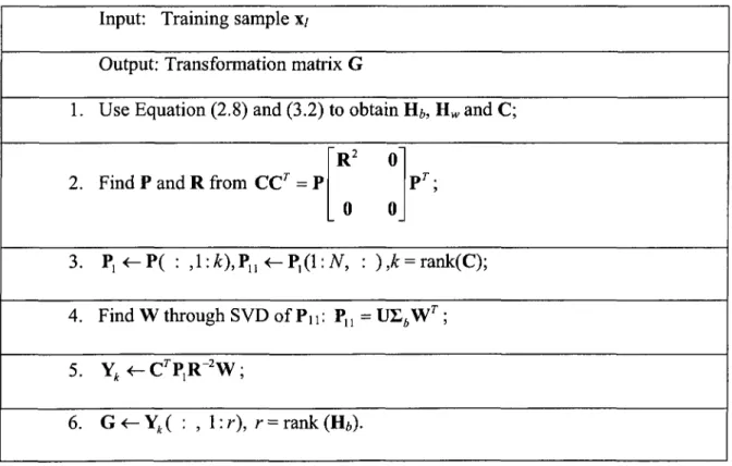
The leftmost r columns of Y^ form the optimal transformation matrix G, where r = rank(Hi). The proposed MGSVD-LDA algorithm is summarized in Table 3.1.

Table 3.1: MGSVD-LDA algorithm Input: Training sample X/

Output: Transformation matrix G

1. Use Equation (2.8) and (3.2) to obtain Hi, Hw and C;

2. Find P and R from CCr = P

R2 0

0 0 Pr;

3. = rank(C);

4. Find W through SVD of Pn: P„ = U£AWr ;

5. Yk <- CrP,R 2W ;

(53)

2 3

Computing SVD of C requires approximately 2m (N+ n)+ l\(N+ n) flops, if Chan's algorithm [78], which is efficient for a matrix with the column dimension much higher than the row dimension (the case of small sample size datasets), is used. On the other

T 3 2

hand, computing the eigen-decomposition of CC needs only 3/4 (N + n) + 0((N + n)) flops [78], which is much smaller than the flop count required form computing the SVD of C. In addition, computing of the SVD of C requires a memory space of approximately

(m + N + n) (N + n) locations, whereas computing the eigen-decomposition of matrix

T 2

CC requires only (N + n) locations. In the case of small sample size datasets, that is,

m » (N+ ri), the proposed MGSVD-LDA algorithm uses much less memory space than

the LDA/GSVD algorithm does. From the above discussion, we conclude that, in the case of small sample size datasets, the proposed MGSVD-LDA algorithm has much lower levels of time and space complexities than that of the LDA/GSVD algorithm.

3.4 Kernelization of MGSVD-LDA

In the preceding section, we have presented a linear discriminant algorithm, which, like most other linear discrimination approaches, assumes that the classes are linearly separable in the input space. However, the distributions of many patterns in the real world are nonlinear, and linear methods of discriminant analysis may not provide sufficient recognition accuracy. Fortunately, in this case one can establish the linear separable condition [87] by using appropriate kernels [55] and then apply the linear discriminant analysis techniques in that space. We now present a scheme to kernelize the proposed MGSVD-LDA algorithm. The new kernel discriminant analysis algorithm is hereafter

(54)

referred to as the MGSVD-KDA algorithm.

As it was done for the development of the MGSVD-LDA algorithm, we first define the following matrix: ® * = I [•^(N>( , ) - V), • • •, V'V0«K(,) - V), • • •, V M V*0 - V)] ( 3 . 2 2 ) and r = o o ( 3 . 2 3 )

where \|/(,) is the centroid of the /'th embedding class, and \|/ is the global centroid of the

embedding samples in the /-dimensional kernel feature space. The SVD of T is given by

r = p

R O 0 0

( 3 . 2 4 )

where P € and Q e W*f are orthogonal matrices, and R e 9?zxz with z =

rank( T ) is a diagonal matrix with its elements being equal to non-zero singular values of r sorted in a non-increasing order. Due to the high dimensionality of T , it would be practically not feasible to conduct the SVD directly. However, the smaller dimension singular vector matrix P and singular value matrix R can be evaluated separately by using the kernel method. We form a symmetric matrix as

r r =

. w b w w .

(55)

where each of the four sub-matrices is in an inner product form. The matrix P is exactly the eigenvector matrix of ITR and the matrix R is the square root of its eigenvalue

matrix. The main problem here is as how to evaluate the matrix I TR, or equivalently, the

four sub-matrices. We construct a kernel matrix

K = ( */ AW , „ ( 3 . 2 6 )

whose elements are the inner products in the feature space determined through a kernel function. Then, we can express the sub-matrices in ( 3 . 2 5 ) in terms of K as

0 [ 0A = D ( B - L )R K ( B - L ) D < D >W = ( I - A ) K ( I - A ) ( 3 . 2 7 ) 0 > [ < I >W= D ( B - L )RK ( I - A ) where A = diag{A,,• • •, AN), A,. = (1 / n , ) ^ B = diag(Bl,-,BN),Bl=(l/ni)lliX,

i = \,---,N, L = (1 / ri)nxN, and I is an n x n identity matrix.

Derivation of this set of formulas is presented in Appendix A.

Similar to the MGSVD-LDA algorithm, the eigen-decomposition of ITR generates

the eigenvector matrix P and the non-zero eigenvalue matrix R . The leftmost z columns

(56)

matrix Pu . The SVD of Pu provides the orthogonal matrices U and W such that

P„ = UZ^W . Letting Yz = rrP,R 2W and A = WrR ^ , we have

Y: = A r (3.28)

Further, let

G = A . r (3.29)

where v = r a n k ( 0r06) , and Av consists of the first v rows of A . The columns of G are the extracted feature vectors of the feature space.

Given a test image x( with its mapping in the feature space being i|/,, the kernel

function is applied again to obtain

q, =k((xl,x,)) = {v„yrl) and subsequently to form the vectors

Q *= x [ - q)' - ' y f i t o1 0 - • • •' V M q("} - q)]

(3.30)

(3.31)

where q(,) =— ]T q, and q = — X"=1q,. Since r\j/r =

n

q r

_{, the projection of}

\|/, on the feature vectors can be found as

w = Gr\|/, = Av

Q[

(3.32)

The proposed MGSVD-KDA algorithm is summarized as in Table 3.2

This algorithm, like many other kernelized algorithms, has a computational complexity determined approximately by the accumulated effects of implementing the

(57)

kernel operator and the associated linear discriminant algorithm with the cost of computing the kernel matrices depending mainly on kernel function chosen.

Table 3.2: MGSVD-KDA algorithm Training stage

Input: Training sample x/ Output: Av in (3.29)

1. Form the kernel matrix K based on (3.26) and (3.26) and the kernel function chosen;

2. Evaluate the matrix I T given by (3.25) using (3.27); 3. Find Pand R from IT7" = P

R2 0

0 0 P ' ; 4. P, P(:,l: z), Pn P,(l: N,:), z = r a n k e r7" ) ;

5. Find W through SVD of P„: P„ = UL.W7 ;

6. Av <- the first v rows of W ' R 2P, , v = rank(0A ) ;

Classification stage Input: Test vector x,

Output: Weight vector w in (3.32); 7. Evaluate q, as in (3.30);

8. Form Q6 and Qwin (3.31);

(58)

3.5 Solving the Over-Fitting Problem

The proposed MGSVD-LDA algorithm, like other GSVD based algorithms, is susceptible to the over-fitting problem. As all the eigenvectors computed in the eigen-decomposition of CCT are maintained and these eigenvectors are divided by the corresponding eigenvalues, as seen from (3.19), the impact of the random features on the eigenvectors corresponding to small eigenvalues gets amplified.

There are mainly three methods to address the over-fitting problem. The first one is a regularization method [31], [33] in which a small positive perturbation is introduced to a matrix in order to bring small changes to large eigenvalues relative to the changes in the small eigenvalues. Thus, the effect of over-fitting can be reduced when the eigenvectors are divided by the eigenvalues resulting from the perturbed matrix. The optimal perturbation parameter is estimated adaptively from the training samples through cross-validation. However, this process is time consuming. In the second method, the smaller eigenvalues and the corresponding eigenvectors are dropped [85]. But, there is no universal criterion to determine as to how many eigenvalues can be considered small enough to be dropped. Both these methods affect the main idea behind the GSVD technique in that the samples of different classes do not converge into distinct compact regions.

The third approach to fixing the over-fitting problem is to orthogonalize the basis of the discriminant subspace [86]. In this method, the basis is orthogonalized through a QR decomposition of G. However, QR decomposition is computational inefficient for high