Development of a Classification Scheme for Managing Human
African Trypanosomiasis using Geospatial Techniques
Akiode Olukemi Adejoke1* Oduyemi Kehinde O K2.
1. School of Science, Engineering and Technology, University of Abertay, Dundee Scotland UK; National Space Research and Development Agency, Abuja, Nigeria.
2. School of Science, Engineering and Technology, University of Abertay, Dundee, Scotland UK *Emails of the corresponding authors: [email protected], [email protected]
Abstract
Distinctive environ-climatic variables have been associated with Trypanosoma brucei gambiense spatial characteristics, signifying the importance of physical landscape in H A T propagation/risk. Nevertheless, techniques projected to classify human African trypanosomiasis (HAT) vector habitats tend to be generalised, time wasting and costly. Despite control efforts, HAT has become resurgent in some locations. No model to acquire detailed and comprehensive HAT spatial or epidemiological data exists for the study area, meaning many of those most in need, especially those residing in remotest parts of the region, may not be benefitting from good health care due to lack of information about them. This paper proposes a geospatial technique to explore vector habitat mapping. The goal was to develop a surveillance methodology t h a t will facilitate quick and efficient management of HAT. Supervised classification and fuzzy logic were integrated to classify land cover and ancillary datasets into HAT vector habitat. The importance of criteria and how they were prioritised were determined by the judgments of experts, the impact of the criteria on HAT propagation and previous studies. Spatial distribution/habitat characteristics play an important role in HAT propagation. Therefore, locations which have all or most of these criteria present are vital for HAT propagation. This study helped distinguish HAT vector habitat into different zones (breed, feed and rest), the classification scheme is expected to offer effective decision support to all stakeholders.
Keywords: Geospatial, Remote Sensing, Geographic Information Systems, Fuzzy, Vector
1. Introduction
Human African Trypanosomiasis (HAT) or ‘sleeping sickness’ is an fatal disease caused by infection by protozoan parasites of the species Trypanosoma brucei. HAT is amongst the top thirteen neglected tropical diseases (NTD) in the world (Hoskins 2009) and is most common in the countries of sub-Saharan Africa (SSA), such as Nigeria and the Democratic Republic of Congo; it currently has limited treatment options. NTDs are often called poverty diseases, as they affect almost exclusively very poor remote populations beyond the reach of health services and are responsible for more than half a million deaths annually (Hoskins 2009; Boutayeb 2007). The HAT parasite is endemic and free-living in the environment, and infection of the human population can be caused either through sexual transmission (Rocha et al. 2004), mother-to-child infection (Olowe 1975) or through insect vectors such as the tsetse fly (Steverding 2008). This study focuses on infection is caused by insect bite.
NTDs are common amongst the poor in SSA, especially in Nigeria and the Democratic Republic of Congo (Hotez & Kamath 2009). HAT affects thousands of people each year, primarily in areas of conflict, where they cause high mortality. There is dearth of information on Africa’s protozoan NTDs and the overall burden of African’s NTDs may be severely underestimated (Hotez & Kamath 2009). Although numbers of cases voluntarily presenting for treatment each year have increased, in Nigeria the exact number of HAT cases is unclear (Abenga & Lawal 2005).
Despite control efforts, HAT has become resurgent in some locations (e.g. Southern Nigeria) and resistance to available medication has been reported in sub-Sahara Africa (Hoskins 2009). The resurgence o f Trypanosomiasis in some endemic foci continues to impact rural development in sub-Saharan Africa. Efforts to control and free these foci from disease have led to introduction of targeted programs. Achieving HAT free foci depends largely on tsetse f l y ecology and suitable vector spatial distribution datasets. Thus, HAT vector habitat maps are indispensable, but, in some endemic regions, this spatial distribution and HAT vector prevalence information is still insufficient for wider area planning and management. To address this issue, requires examination of how land cover datasets may influence HAT vector habitat mapping.
1.1 HAT Distribution Mapping: Previous Efforts
used to assess the spatial distribution boundary of various types of HAT vector (Katondo 1984). Lately, geospatial techniques such as, RS and GIS have been used in mapping tsetse distribution at varying scales (Courtin et al. 2005; De Deken et al. 2005). In spite of this progress, the level of detail and accuracy of some of the existing HAT vector spatial distribution maps/datasets, are still not sufficient for the scheduling and execution of wide area surveillance programmes.
It is also obvious from the literature that the physical landscape is very important to HAT propagation; yet, few efforts have been made to pinpoint the exact locations where HAT patients are infected. Geographic unit to which disease datasets were linked were generalized, even though this type of landscape analysis will not permit the detection of highly HAT hazardous locations. It is very important that the landscape within HAT endemic areas is well characterised. These studies, irrespective of their level of details, accuracy, and original goals have served as basis for HAT control programmes across sub-Sahara Africa. However, due to the heterogeneous nature of the sub-Sahara Africa environment and the importance - economic or otherwise - of varying biotic and abiotic components, HAT management and controlling activities will benefit from detailed landscape characterisation studies.
Underreporting is one of the factors affecting HAT (Osue et al. 2008). Underreporting of HAT cases, most especially T. b. gambiense, is an indication that supplementary data gathering approaches, other than the existing active and passive case surveillance, are required. The existing case surveillance methods are insufficient to fully describe the extent of HAT. While infected people may not access passive surveillance facilities for treatment until a late stage, due to the asymptomatic nature of the West African form of HAT, the active surveillance team may not detect the case because of constraints such as limited resources a nd t he nature of the terrain etc. This results in underreporting and eventually resurgence of the disease. To overcome the limitations of the existing system as well as promote improved HAT management; the integration of geospatial techniques is very important.
1.2 Geospatial Techniques in Disease Mapping
Geospatial techniques such as Remote Sensing (RS) and Geographic Information Systems (GIS) have permitted epidemiologists to perform disease mapping and spatial analyses (Symeonakis, Robinson & Drake 2007). A better understanding of the dynamics of disease propagation in a population and the spatio-temporal variations in disease incidence provides a basis for effective disease control (Kelly-Hope & McKenzie 2009). However, spatial aspects of HAT are rarely addressed, and most HAT studies, particularly in the Delta State of Nigeria - the research area of this study, are based on medical diagnostics (Wang et al. 2008). In Nigeria, the existing HAT surveillance system and the establishment of precise demarcation of the disease magnitude is limited by unstable security (Simarro et al. 2010).
Conscious of the constraints in managing HAT in sub-Sahara Africa, the World Health Organisation (WHO) granted exclusive support to some HAT endemic nations, including Nigeria, in order to improve epidemiological understanding and establish innovative disease management tools (Simarro et al. 2011). Geospatial techniques such as RS, GIS and spatial statistics were implemented and have been shown previously to be effective in developing efficient disease management (Hotez & Kamath 2009). These techniques have also been used previously for monitoring HAT (DeVisser &Messina 2009; Symeonakis, Robinson & Drake 2007). This approach will contribute to both t h e local and international understanding o f how best to manage HAT propagation in study area with poor security (Symeonakis, Robinson & Drake 2007) as well as provide insights into the underlying factors affecting the disease.
Reversing the trend of HAT resurgence is a key challenge and v ector control will be necessary to disrupt propagation. The present study will carry out a detailed characterisation of the study area environment (at a regional scale) using geospatial-fuzzy multi-criteria d e ci s i o n a na l ys i s to identify and classify potential HAT vector habitats into zones, to ease disease management.
1.3 Geospatial Multi-criteria Decision Analysis
Spatial decision problems usually involve a large set of viable options and several evaluation criteria, which are often weighed by multiple stakeholders with conflicting interests (Tsiko & Haile 2011). Thus, factors to be considered while developing efficient strategies to manage HAT or vector-borne diseases are many, and the
a relational scale (Saaty 1980) to determine their relative significance.
Fuzzy membership function has been used to improve the uncertainty associated with AHP decision (Buckley 1985). Fuzzification, according to Erensal et al. 2006, can capture the uncertainty inherent in complex multi-attribute decision analysis problems. Fuzzy theory permits the membership functions to function over a range of real numbers [0, 1] to delineate the extent or strength of membership of element(s) in a fuzzy set.
The use of fuzzy logic to integrate ancillary datasets with land cover to improve classification had been attempted in the past (Gopal et al. 1999), however, it had not been used to delineate HAT vector habitat into different zones. The application of geospatial-fuzzy MCDA to disease epidemiology is also becoming popular, with past studies demonstrating its effectiveness (Wang and Wang 2010; Rajabi, Mansourian & Bazmani 2012). Zoning the potential vector habitat could permit both quick preventative and diagnostic management of HAT. The rationale for classifying the HAT vector habitat is based on studies that emphasised their significance to vector survival and HAT resurgence. (DeVisser & Messina 2009; Goetz et al. 2000).
1.4 The Study Region: The Niger Delta Nigeria
Nigeria is a large country in West Africa, of over 900 000 square kilometres and is the most densely populated country in Africa (140,431,790; Nigeria National Population Commission 2006). The Niger delta region is one of the five geopolitical zones in Nigeria (Figure 1) and is one of the world’s largest wetlands.
Figure 1: Nigeria geopolitical zones (from: www.naijanedu.com/the- 19-new- proposed-states-to-be-created-in-nigeria/
The region is mainly vegetated by mangrove forests, the largest in Africa (Ibe 1998). The climate is characterised by high humidity (between 90% and 100%) and heavy rain falls (annual average is between 2500-3550 mm). The annual mean temperature is 26oC, but fluctuates seasonally between 21-33 oC, (Leroux 2001). These humid and hot conditions are favourable for HAT vector survival ( Courtin et al. 2005). The predominant occupations include farming, fishing and hunting (Niger Delta Environmental Survey 1997). These activities exacerbate HAT propagation as the population is exposed to the disease vector on daily basis. The main study area selected for this research work comprises two local government areas (Ethiope-east and Ukwuani) within Delta state (Delta State is one of the states that comprises Niger delta region), which were chosen as they have been identified as active HAT foci, and records indicated continuous HAT positive cases (Osue et al. 2008; Abenga and Lawal 2005). The region that is located between latitudes 5o30’N and longitude 6o00’E (Figure 2), is remote and rural, and HAT has been linked to populations living in areas beyond the reach of health services (Boutayeb 2007), a situation compounded by the terrain and continuous conflicts within the region, which pose difficulties for health care delivery. The area is, however, economically important to the state, both in term of resources and human capital.
The 2008 WHO initiative to map all reported HAT cases at village level (Simarro et al. 2011), is difficult due to restricted disease surveillance and access to diagnoses. No model to acquire detailed and comprehensive spatial or epidemiological data exists for the study area, meaning many of those most in need, especially those residing in remotest parts of the region, may not be benefitting from good health care due to lack of information about them. It is thus imperative to develop a HAT v e c t o r habitat classification
scheme that can be applied to identify high-priority areas where surveillance and health care delivery should be directed.
Figure 2. The Delta State of Nigeria
2. Materials and Methods
All the data used were projected to the World Geodetic System (WGS) 84 datum Universal Transverse Mercator (UTM) Zone 32N. Using Global Positioning Systems (GPS), ground control points (GCPs) for settlements in the study area were collected, exported into ArcMap and converted into shape files using the same coordinate systems as the other spatial data. Geospatial-fuzzy MCDA was applied at every stage of the research work particularly in delineating HAT vector habitat. The remote sensing images used in this study are presented in Table 1 and the criteria (Table 2) used in this study were derived manly from the RS images.
Table 1: Remotely sensed data used in this study
Data Type Acquisition Date Path/Row Bands used Spatial Resolution (m) Source Landsat7 30/12/2002 189/56 2, 3, 4, 30 LP DAAC
2.1 Methods
2.1.1 Image Processing
The Landsat 7 ETM+ image was preprocessed to reduce or eliminate errors embedded in the data due to sensor effects, atmospheric and illumination effects as well as mis-registration. Both geometric and atmospheric corrections were carried out to derive the environ-climatic (Table 2) criteria required for this study from the RS image. The algorithms (equations) used are presented in the appendix .
Geometric Correction: using IDRISI Selva 17.0 software, the DEM data used for this study was re-sampled to 30 metres from 3-arc seconds (approximately 90 metres) using the 2002 Landsat ETM+. The root mean square error (RMSE) output for the DEM was about 0.42 indicating a good re-sampling.
Atmospheric correction: using image-based dark object subtraction method, the digital number (DN) of the image bands were converted to at-satellite spectral radiance and from at-satellite spectral radiance to top-of-atmosphere (TOA) reflectance. The at-satellite spectral radiance data (all image bands) was derived using Equation1 while the TOA reflectance data was derived for all the image bands (excluding thermal band) using Equation 2. All the parameters used are contained in the image metadata file.
The at-satellite spectral radiance and TOA spectral reflectance data derived were transformed to retrieve land surface temperature (LST), normalized difference vegetation index (NDVI), normalized difference water index (NDWI), and relative humidity (RH), using appropriate algorithms (see appendix). To derive land surface temperature (LST), the spectral radiance value of thermal band of the 2002 image was converted to at-satellite brightness temperature using Equation 3. Because at-satellite brightness temperature only represents blackbody temperature, it was corrected for spectral emissivity (land surface emissivity) before estimating LST using equation 4. NDVI (Equation 5), was retrieved using the near-infrared (band 4) and red (band 3) components of the Landsat 7 ETM+ while NDWI (Equation 6) was extracted from the images because it is required to estimate normalized difference drought index (NDDI). The NDDI was estimated using Equation 7. Meteorological data obtained from Nigerian Meteorological Agency (NIMET), was combined with the LST to derive relative humidity (RH) us i ng Equation 8.
All the criteria derived from the RS image were stored in a personal geodatabase. An analytic hierarchy process (AHP) questionnaire survey was carried out to compare the relative importance of the criteria in relation to each HAT vector habitat zone. In order to ascertain the likelihood that the weights obtained from the experts (35 in total; comprises of epidemiologists, geographers, HAT regulatory/coordinating and evaluator bodies) was randomly generated, the weights consistency ratios were calculated. The consistency ratios (CR) were less than 1 thus, consistent. According to Saaty (1980), any CR up to 0.10 is considered satisfactory. The individual priority weights obtained from experts were then aggregated using geometric mean to obtain the overall priority weight for each criterion.
2.1.2 Image classification
Supervised maximum likelihood classification algorithm was used for land cover classification in ArcMap 10.0 software. To select appropriate image bands for colour composites, principal component analysis (PCA) was carried out. This was to ensure that the satellite image bands used for colour composite have low correlation so as to reduce problem due to linearity. Bands 7, 5 and 2 were selected from the Landsat 7 ETM+ image for the land cover classification.
Adequate number of representative training samples are vital for s upervised image classifications (Chen and Stow 2002). Several training samples were collected from areas that appeared relatively similar on the 2002 Landsat 7 ETM+ image. Groundtruth data, previous knowledge of the study area aid the training set samples. The next step was the generation of signature file. This is the statistical description of the classes; t hese statistics are required for the supervised classification. After the creation of signature file, the maximum likelihood classification (supervised classification) was carried out. For the supervised classification, the colour composite image (bands 7, 5, 2) was used as input raster bands, and the signature file created for the training samples served as input signature file. A total of 7 land cover classes, as shown in Figures 3 were identified.
2.1.3 Post-classification processing
The seven classes in the supervised classified image were separated into separate layers, after which the built-up area layer was generalised. This was done using the ArcMap 10.0 region grobuilt-up tool set to reclassify the small isolated regions of the built-up area pixels to the nearest class. This enables each settlement in the study area to be identified as a separate entity, rather than a class in the domain type land cover.
Figure 3: Supervised land cover classes in the study area (source: 2002 Landsat 7 ETM+ and groundtruth)
2.1.4 Image classification accuracy assessment
To evaluate the result of the classification, the spectral characteristics of the classes represented by the training samples were assessed. Also, to ascertain the accuracy of the classification, t h e error matrix was computed using GCPs obtained during ground thruthing. The classified output was also compared with a high resolution spot image obtained from Google Earth. The Spot image shows more detail than the Landsat image used as the base data for the classification. To check the extent to which there is agreement other than that which is expected by chance, kappa statistics was also calculated for the supervised classification.
2.1.5 Development of a classification scheme for managing HAT
This section focuses on combining the land cover classes and other derived environmental/climatic variables (section 2.1.1) to develop a classification scheme. The importance of criteria and how they were prioritised were determined by the judgments of experts, the impact of the criteria on HAT propagation and previous studies. Spatial distribution/habitat characteristics play an important role in HAT propagation. Therefore, locations which have all or most of these criteria present are vital for HAT propagation. To achieve the goal of this section, geospatial-fuzzy MCDA was used. The overall goal is to identify and classify HAT vector habitat in the study area into different zones, namely: breed, feed and rest zones to aid efficient management of HAT. Thus, a hierarchical structure was created with the goal, criteria/sub-criteria and alternatives (Figure 4).
Figure 4: Hierarchical structure of goal, criteria and alternatives
The selection of criteria is a vital procedure in geospatial-fuzzy MCDA. Criteria used in the HAT vector habitat classification scheme were categorised into two: Land cover classes and ancillary datasets. These two criteria were separated into sub-criteria for clarification purposes, as highlighted in Table 2 . The criteria were jointly chosen by the researcher and experts to ensure suitability for the classification scheme. Some decision rules were applied to manipulate the criteria to obtain the alternatives.
Table 2: Criteria for classification of HAT vector habitat
Major Criteri
a
Sub-Criteria Unit Source
A N CI L L A R Y DATAS E T S Land surface temperature Relative humidity Digital terrain model NDVI NDDI Degree Celsius % Meters Index Index Landsat 7 ETM+ Landsat 7ETM+/NIMET SRTM Landsat 7 ETM+ Landsat 7 ETM+ L A ND CO VE R CL ASSE S Water body Mangrove Less dense forest Dense forest Cultivated area Shrub Built-up area % % % % % % % Landsat 7 ETM+ Landsat 7 ETM+ Landsat 7 ETM+ Landsat 7 ETM+ Landsat 7 ETM+ Landsat 7 ETM+ Landsat 7 ETM+
2.1.5.1 Geospatial-fuzzy Multi Criteria Decision Analysis
All the criteria (land cover and anxillary) were stored in a personal geodatabase. An AHP questionnaire survey was carried out to compare the relative importance of the criteria in relation to each HAT vector habitat
Ancillary Datasets
Classification of HAT Vector Habitat
into Zones
Land Cover
Classes
Breed Zone
Feed Zone
Rest Zone
Goal:
Criteria
:
zone. In order to ascertain the likelihood that the weights obtained from the experts was randomly generated, the weights consistency ratios (CR) were calculated. Each expert’s AHP matrix was entered into IDRISI software to obtain priority vector and consistency ratio. The consistency ratios were less than 1 thus, consistent. The individual priority weights obtained from experts were then aggregated using the geometric mean to obtain the overall priority weight for each criterion.
2.1.5.2 Grouping of study area into HAT vector habitat zones
Geospatial-fuzzy multi criteria decision analysis was carried out to group the study area into HAT vector habitat zones.
The supervised land cover classes obtained were reclassified into three ( breed, feed and rest) temporary HAT vector habitat zones. Also, the derived ancillary datasets were grouped into each habitat zone using a weighted sum. The reclassification of the land cover and grouping of the ancillary datasets were done using the weights obtained from the experts. The temporary HAT habitat zones were fuzzified and combined with fuzzified weighted ancillary datasets to obtain the final HAT vector breed, feed and rest zones. The fuzzification was carried out using fuzzy membership type ‘large’ whereby large values of the input map criteria layer have high membership in the fuzzy set (further detail in ArcMap 10.0 help). The fuzzification was necessary partly to normalise the criteria into common scale and also to obtain their fuzzy membership sets. The process used is presented in Figure 5. Before choosing the final HAT vector habitat zones, sensitivity analysis was carried out. The weights of the ancillary datasets obtained for each zone from experts, were changed as follows:
Equal weight: Each criterion was assigned 0.2 values before calculating their weighted sum.
Five percent weight increase: Each criterion’s weight was increased by 5% before calculating their weighted sum.
Ten percent weight increase: Each criterion’s weight was increased by 10% before calculating their weighted sum.
After the weight change and the calculation of weighted sum, each outcome map layer (for each zone) was overlaid on the corresponding HAT vector habitat temporary zones. The overlay analysis was done using fuzzy overlay operator ‘OR’ ‘AND’ and ‘GAMMA’. The overlay type ‘OR ‘was carried out using fuzzy maximum operator to generate map layer that contained maximum fuzzy membership value for locations within each HAT vector habitat zone, while the fuzzy overlay operator ‘AND’ returns map layers showing minimum membership values for all location within each HAT vector habitat zone. For the final identification and classification of the HAT vector habitat zones, different fuzzy overlay operator gamma values were used. This was to investigate the appropriate value that will not change considerably the original ancillary weights obtained from the experts.
Figure 5: Habitat grouping procedure
2.1.6 Validation of HAT Vector Habitat Classification Scheme
Geo-statistical analysis was carried out to make decision as to whether the classification scheme values could be practical.
2.1.6.1 Semivariogram sensitivity analysis
After obtaining the final HAT vector habitat zones, the output map layers were defuzzified. This was necessary so as to be able to perform sensitivity analysis on the data. Using the predicted values and standard errors of the defuzzified map layers obtained from kriging geo-statistical analysis, semivariogram sensitivity analysis was performed (in ArcMap 10.0) by changing the kriging model’s parameters; such as, partial sill and nugget within the percentage of the initial values. The initial nugget and partial sill for each HAT vector habitat zone were changed using 5%, 10%, 15% and 20% nuggets and partial sills.
Weighted sum map
Land cover classes
NDVI, NDDI, LST,
DEM, RH
Reclass Landcover
using weight
using weight
Weighted sum
Temporary habitat zones
(Breed, Feed, Rest)
Reclass
weighted sum
Fuzzify
Reclass Map Fuzzy Membership
(Breed, Feed,Rest)
Fuzzify
y
Overlay
Fuzzy MembershipHabitat Zones (Breed,
Feed, Rest)
2.1.6.2 Local polynomial interpolation quality of fit analysis
Local polynomial interpolation (LPI), which provides spatial condition number surface, was performed. Spatial condition number surface is a measure of stability and reliability of the outcome of a prediction equation for a given location. The rules of thumb for critical values for spatial condition number surface are: for 1st order polynomial, the threshold is 10, 2nd polynomial order threshold is 100 while 3rd order polynomial has 1000 critical threshold (ArcMap 10.0 help). The LPI surface was derived for each HAT habitat zone to form a geo-statistical layer for cross-validation using a 1st order polynomial transformation. Empirical Bayesian kriging (EBK) was also carried out to assess the quality of fit of the classification models. The main reason for EBK was to use a more accurate method; E B K standard errors of prediction are more accurate than LPI measurement.
3. Results
The evaluation of the image classification training samples shows that they were representative for the study areas and are statistically separate. The histograms of the land cover classes did not overlap. The overall accuracy of the image classification was 9 9 . 2 % (Tables 3). All the identified land cover class have 100% producer and user’s accuracy, except for cultivated areas and shrub that have 94.59% and 94.29% producer’s and user’s accuracy, respectively. This may be due to the spectral reflectance of shrub similar to less dense forest reflectance and some matured/tall plants within the cultivated class in some areas. The overall kappa statistics (Table 4) was 0.9907; this is an indication of strong agreement between the classified pixels and the reference data.
Table 3: Error matrix for study area supervised land cover classification
Class Reference Classified Number Producers Users Name Totals Totals Correct Accuracy Accuracy
--- --- --- --- --- --- Unclassified 0 0 0 --- --- Dense Forest 37 37 37 100.00% 100.00% Mangrove 35 35 35 100.00% 100.00% Less Dense Fore 37 37 37 100.00% 100.00% Shrub 33 35 33 100.00% 94.29% Built-up Area 36 36 36 100.00% 100.00% Cultivated Area 37 35 35 94.59% 100.00% Water Body 35 35 35 100.00% 100.00% Totals 250 250 248
Overall Classification Accuracy = 99.20%
Table 4: Kappa statistics for study area supervised classification
--- --- Unclassified 0.0000 Dense Forest 1.0000 Mangrove 1.0000 Less Dense Forest 1.0000 Shrub 0.9342 Built-up Area 1.0000 Cultivated Area 1.0000 Water Body 1.0000
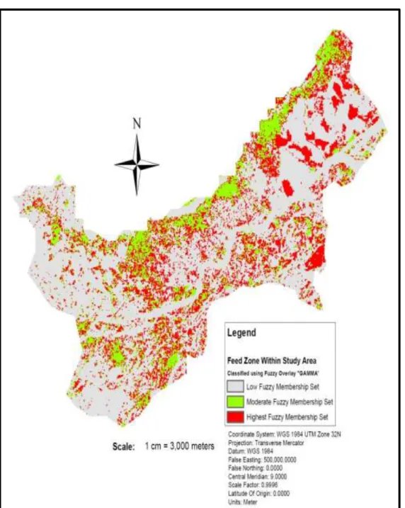
The area of fuzzy membership categories (low, moderate and high) did not change considerably from the area estimated with the weights obtained from experts, when using fuzzy gamma operator values ranging from 0.1 to 0.8. However, gamma value above 0.8 decreased the area estimates considerably. Thus fuzzy values in the 0.1 to 0.8 range appear to be suitable gamma values for combining the fuzzy membership sets of the HAT vector temporary habitat zones and the ancillary datasets towards the final HAT vector habitat zones. The final HAT vector habitat zones were generated using a value of 0.8, as it was the most consistent value in that range. Figures 6, 7 a n d 8 shows the final HAT vector habitat zones, while Table 5 shows the result obtained using a gamma value 0.8 and fuzzy overlays ‘OR’ and ‘AND’,
The final selection of locations for each zone was based on the gamma overlay operator outcome, because the fuzzy overlay operators OR and AND only utilised the maximum and minimum fuzzy membership values of the criteria. Since, the essence of this study is to identify all possible HAT vector habitats in the study area; fuzzy overlay operator gamma was adopted. The use of gamma overlay type produced output values that ensure a flexible compromise between the two extremes (minimum and maximum).
Figure 6: HAT vector breed zone within the study area classified using
fuzzy overlay operator ‘GAMMA’
Figure 7: HAT vector feed zone within the study area classified using fuzzy
overlay operator ‘GAMMA’
Figure 8: HAT vector rest zone within the study area classified using fuzzy
overlay operator ‘GAMMA’
Table 5: Summary of sensitivity analysis used to verify the weights of
criteria assigned by experts
___________________________________________________________________________
Fuzzy Operator Weight of Criteria Zone Category (Area %)
LFM MFM HFM
Overlay OR Experts - 65 35
Overlay AND Experts 65 28 7
=fuzzy overlay operator Gamma, 0.8 = fuzzy gamma value LFM = low fuzzy membership set,
MFM = moderate fuzzy membership set HFM = highest fuzzy membership set..
The semivariogram analysis revealed very minute variation in the original data (habitat zones). It was observed that with increased distance from a given location, the nugget for that location reduces while the partial sill for the same location increases. Though variations were observed with the semivariogram sensitivity analysis, the variations were between 0.0 – 0.1%, thus, the researcher has high confidence in further application of the newly developed HAT vector habitat classification scheme. The spatial condition number obtained (from LPI) for each habitat zone was below the critical threshold value o f 10, thus the model can be regarded as reliable and stable. The outcome of the LPI and EBK (Figures 9-11)cross validation for each habitat zone produced mean and standardised mean prediction errors that was near zero, this was an indication of unbiased prediction that was centred on true values. The scatter plot of the cross-validation analysis revealed three and one data locations that were set aside from all the other locations in the Breed and Rest zone respectively. Ideally, this should have called for the autocorrelation models to be refit with misfit data removed. However, the data was retained to truthfully represent real world relationships and not an existing theory ____________________________________________________________________________ ____________________________ BREED ZONE_______ BREED ZONE 𝛾 = (0.8) Experts 38 27 35 Equal weights 31 32 37 10% increa 5% increase weights 35 30 35 _____________________________________________________________________________ FEED ZONE Overlay AND Experts 69 11 22Overlay OR Experts 7 75 18 𝛾 = (0.8) Experts 64 14 22 Equal weights 56 22 22 5% increase weights 62 16 22 10% increase weights 63 15 22 REST ZONE Overlay AND Experts 71 28 1
Overlay OR Experts - 19 81
𝛾 = (0.8) Experts 30 36 34
Equal weights 30 55 15
5% increase weights 33 31 36
Figure 9: Quality of fit assessment of HAT vector breed zone in the
study area using empirical Bayesian kriging
(source: Cross validation
analysis (Note: simulated semivariogram insert))
Figure 10: Quality of fit assessment of HAT vector feed zone model
in the study area using empirical Bayesian kriging
(source: Cross
validation analysis)
Figure 11: Quality of fit assessment of HAT vector rest zone model in the study area using empirical Bayesian kriging (source: Cross validation analysis)
4. Discussion and Conclusion
The aim of this study was to carry out a detailed characterisation of the study area environment (at a regional scale) using geospatial techniques to identify and classify potential HAT vector habitats into zones, to ease disease management. The use of geospatial techniques in developing the classification scheme was successful. The criteria used for this study were derived from RS images because of dearth of digital data/information in the study area. The semivariogram analysis and the best fit analysis showed that the classification model was reliable and practical. The integration of supervised classification and fuzzy logic have not been previously used with land cover classes and remotely derived continuous ancillary data to map out vector habitat zones, at the level of thematic detail shown here. Therefore, the present research work is unique.
the basic settings for effective management of the disease, particularly in the study area and in sub-Sahara Africa. Unlike previous studies, however, the approach used in this study has helped to distinguish (though containing fuzzy boundaries) the HAT vector habitat into three zones. Delineating the vector habitat into zones can help to precisely identify the direction and magnitude of HAT, the factors influencing HAT propagation, and the priority areas in the study area, as well as identifying the areas with least chance of HAT propagation. This suggests that geospatial techniques may be valuable where epidemiological data/information are limited, to allow precise analyses to be carried out regarding the spatial propagation of a disease. The technique used in this study can be adapted to map other vector borne diseases habitat.
References
Abenga, J. N. & Lawal, I. A. ( 2005), “Implicating roles of animal reservoir hosts in the resurgence of Gambian trypanosomiasis (sleeping sickness)”. African Journal of Biotechnology. 4(2): pp. 34-137.
ArcGIS 10.0 Desktop help. [No Date]. Available from:
http://help.arcgis.com/en/arcgisdesktop/10.0/help/index.html#//00v20000000t000000.htm
Boutayeb, A. (2007), “Developing countries and neglected diseases: challenges and perspectives”. International Journal for Equity in Health. 6(20).
Buckley, J. J. (1985), “ Fuzzy hierarchical analysis”. Fuzzy Sets and Systems. 17(3): pp. 233-247. Chander, G., Markham, B. L.& Helder, D. L. ( 2009), “ Summary of current radiometric calibration
coefficients for Landsat MSS, TM, ETM+,and EO-1 ALI sensors”. Remote Sensing of Environment. 113: pp. 893–903.
Chen, D. & Stow, D. A. (2002), “The effect of training strategies on supervised classification at different spatial resolution”. Photogrammetric Engineering and Remote Sensing. 68: pp. 1155–1162.
Courtin, F., et al. 9 2005), “ Towards understanding the presence/absence of human African trypanosomosis in a focus of Cote d'Ivoire: a spatial analysis of the pathogenic system”. International Journal of Health
Geographics, 4 (27). doi:10.1186/1476-072X-4-27.
De Deken, R., et al.(2005),” Trypanosomiasis in Kinshasa: distribution of the vector, Glossina fuscipes quanzensis and risk of transmission in the peri-urban area”. Medical and Veterinary Entomology. 19 (4): pp. 353 – 359.
DeVisser, M. H. & Messina, J. P. (2009), “Optimum land cover products for use in a Glossina-morsitans habitat model of Kenya”. International Journal of Health Geographics: 8(39). doi:10.1186/1476-072X-8-39. Erensal, Y. C., Oncan, T., & Demircan, M. L. (2006), “Determining key capabilities in technology management using fuzzy analytic hierarchy process: A case study of Turkey”. Information Sciences. 176: pp. 2755– 2770.
Goetz, S. J., Prince, S. D., & Small, J. (2000), “Advances in satellite remote sensing of environmental variables for epidemiological applications”. Advances in Parasitology. 47: pp. 289–307.
Gopal, S., Woodcock, C. E. & Strahler, A. H. ( 1999), “F u z z y neural network classification of global land cover from a 10 AVHRR data set”. Remote Sensing of Environment. 67: pp. 230–243.
Hoskins, K. (2009), VaccineEthics.org- “The Ethical Challenges of Vaccine: Neglected Tropical Disease
Vaccine Candidates and Financing” .© 2005 2005—2009, University of Pennsylvania Center for
Bioethics. Available from:
http://www.vaccineethics.org/issue_briefs/ntd_candidates.php.
Hotez, P. J. & Kamath, A. (2009), “Neglected tropical diseases in sub-Saharan Africa: review of their prevalence, distribution, and disease burden”. PLoS neglected tropical diseases. 3(8): e412. Ibe. A. C. ( 1998), “Coastline Erosion in Nigeria.Ibadan”: University press. p. 217.
Irish, R. (2008), “Calibrated Landsat digital number (DN) to top of atmosphere (TOA) reflectance conversion”. Available from:
http://igett.delmar.edu/Resources/Remote%20Sensing%20Technology%20Training/Calculation-DN_to_Reflectance_Irish_20June08.pdf
Ji, L., Zhang, L. & Wylie, B. (2009), “Analysis of dynamic thresholds for the normalized difference water index”. Photogrammetric Engineering & Remote Sensing. 75(11): pp. 1307– 1317.
Katondo, K.M. (1984), “Revision of second edition of tsetse distribution maps”. Insect Science and its Application, 5: pp. 381 – 384.
entomological inoculation rate measurements and methods across sub-Saharan Africa”. Malaria Journal: (8)19.
Landsat 7 Science data users handbook. (2011), “Conversion to Radiance”. Available from: http://landsathandbook.gsfc.nasa.gov/data_prod/prog_sect11_3.html.
Lawrence, M. G. (2005), “ The relationship between relative humidity and the dew point temperature in moist air: a simple conversion and applications”. Bulletin of the America Meteorological. Society. 86: pp. 225–233.
Leroux, M. (2001), 2The meteorology and climate of tropical Africa”. Chichester, UK: Praxis Publishing Ltd. p. 548. Malczewski 1999
Mendoza, G. A. & Prabhu, R. (2000), “Multiple criteria decision making approaches to assessing forest sustainability using criteria and indicators: a case study”. Forest Ecology and Management, 131(1-3): pp. 107-126.
Nigeria National Population Commission. (2006), “2006 population and housing census priority tables”. p. 1. Niger Delta Environmental Survey. (1997), “Environmental and socio economic characteristics”. Lagos:
Environmental Resources Managers, Nigeria.
Olowe, S. A. (1975), “A case of congenital trypanosomiasis in Lagos”. Transactions of the Royal Society of Tropical Medicine and Hygiene. 69 (1): pp. 57–9.
Osue, H. O., et al. 2008), “ Active Transmission of Trypanosoma brucei gambiense dutton, 1902 sleeping sickness in Abraka, Delta State, Nigeria”. Science World Journal: 3(2).
Rajabi, M, Mansourian, A. & Bazmani, A. ( 2012), “Susceptibility mapping of visceral leishmaniasis based on fuzzy modelling and group decision-making methods”. Geospatial Health, 7(1): pp. 37-50.
Rakotomanana, F. et al. (2007), “Determining areas that require indoor insecticide spraying using multi criteria evaluation, a decision support tool for malaria vector control programmes in the Central Highlands of Madagascar”. International Journal of Health Geographics: (6)2.
Renza, D., et al. ( 2010), “ Drought estimation maps by means multidate landsat fused images”. In: 30th EARSeL Symposium: Remote Sensing for Science, Education and Culture, 31/05/2010 - 03/06/2010, Paris, Francia
Saaty, T. L. ( 1980), “The analytic hierarchy process”. McGraw-Hill International, New York, NY, U.S.A. Simarro, P. P., et al. (2010), “The atlas of human African trypanosomiasis: a contribution to global mapping of
neglected tropical diseases”. International Journal of Health Geographics: (9)57. doi: 10.1186/1476-072X-9-57.
Simarro, P. P., et al. (2011), “The human African trypanosomiasis control and surveillance programme of the world health organization 2000–2009: The way forward”. PLoS neglected tropical diseases. 5(2): e1007. doi:10.1371/journal.pntd.0001007.
Steverding, D. (2008), “The history of African trypanosomiasis”. Parasites & Vectors, 1(3). Available from: doi: 10. 1186/1756-3305-1-3.
Suedel, B. C., Kim, J. & Banks, C. J. (2009), “Comparison of the direct scoring method and multi-criteria decision analysis for dredged material management decision making”. DOER Technical Notes
Collection (ERDC TN-DOER-R13).Vicksburg, MS: U.S. Army Engineer Research and Development
Center. Available from: http://el.erdc.usace.army.mil/.
Symeonakis, E., Robinson, T. & Drake, N. (2007), “ GIS and multiple-criteria evaluation for the optimisation of tsetse fly eradication programmes”. Environmental Monitoring and Assessment 124(1-3): pp. 89-103. Tsiko, R. G. & Haile, T. S. (2011), “Integrating geographical information systems, fuzzy logic and analytical
hierarchy process in modelling optimum sites for locating water reservoirs. A case study of the Debub district in Eritrea”. Water. 3(1): pp. 254-290. doi:10.3390/w3010254.
Weng, Q., Lu, D. & Schubring, J. (2004), ”Estimation of land surface temperature vegetation abundance relationship for urban heat island studies”. Remote Sensing of Environment. 89: pp. 467-483.
Appendix
Equation s used in the study
Equation1
(Landsat 7 science data users handbook):
L
λ=Grescale*QCAL+Brescale
Where: L
λ
= spectral radiance at the sensor's aperture in watts/ (metersquared *ster*µm), Grescale =
rescaled gain in watts/(metersquared * ster * μm)/DN,
Brescale = rescaled bias (offset) in
watts/(metersquared * ster*µm), QCAL = the quantized calibrated pixel value in DN.
Equation 2
(Irish 2008; Chander et al. 2009):
𝑃𝜆 = 𝐸𝑆𝑈𝑁𝜆∗ 𝐶𝑂𝑆𝜗𝑠𝜋 ∗ 𝐿𝜆∗ 𝑑2
Where:
𝑃
𝜆= TOA reflectance (no unit),
𝜋
= Pi approximately equal to 3.14159 (no unit),
𝐿
𝜆=
Equation 3.34, d = Earth-Sun distance (astronomical units] (Appendix A-4a),
𝐸𝑆𝑈𝑁
𝜆= mean
exoatmospheric solar irradiance (watts/(meter squared *ster*µm) (Appendix A-4b i, ii, iii),
𝐶𝑂𝑆𝜗
𝑠=
solar zenith angle (degree). Solar zenith angle = 90
0– solar elevation angle (solar elevation angle is
in the accompany image metadata file).
Equation 3
(Chander et al. 2009):
T= K2 / ln(K1/ L
λ)+1
Where:
T
= effective at-satellite temperature in Kelvin, K1 &
K2
= Landsat calibration constants 1 &
2(Appendix A-3b), L
λ = at-satellite spectral radiance,
ln = natural log.
Equation 4
(Weng, Lu and Schubring 2004):
LST =
𝑇1+(𝜆∗𝑇𝜌)1𝑛𝜀