Alduais, N.A.M., Abdullah, J., Jamil, A. and Heidari, H. (2017)
Performance evaluation of real-time multivariate data reduction models for
adaptive-threshold in wireless sensor networks.
IEEE Sensors Letters
, 1(6),
7501204.(doi:
10.1109/LSENS.2017.2768218
)
This is the author’s final accepted version.
There may be differences between this version and the published version.
You are advised to consult the publisher’s version if you wish to cite from
it.
http://eprints.gla.ac.uk/150648/
Deposited on: 12 July 2018
Enlighten – Research publications by members of the University of Glasgow
Sensor Networks____________________________________________________________
Performance Evaluation of Real-Time Multivariate Data Reduction Models for
Adaptive-Threshold in Wireless Sensor Networks (WSNs)
N. A. M. Alduais
1*, J. Abdullah
1**, A. Jamil
1and H. Heidari
2†1 Wireless and Radio Science Centre(WARAS), Faculty of Electrical and Electronic Engineering, Universiti Tun Hussein Onn Malaysia
(UTHM), Parit Raja, Batu Pahat, Johor, Malaysia
2 School of Engineering, University of Glasgow, Glasgow G12 8QQ, United Kingdom
* Student Member, IEEE ** Member, IEEE
† Senior Member, IEEE
Received 1 Nov 2016, revised 25 Nov 2016, accepted 30 Nov 2016, published 5 Dec 2016, current version 15 Dec 2016. (Dates will be inserted by IEEE; “published” is the date the accepted preprint is posted on IEEE Xplore®; “current version” is the date the typeset version is posted on Xplore®).
Abstract— This paper presents a new metric to assess the performance of different multivariate data reduction models in wireless sensor networks (WSNs). The proposed metric is called Updating Frequency Metric (UFM) which is defined as the frequency of updating the model reference parameters during data collection. A method for estimating the error threshold value during the training phase is also suggested. The proposed threshold of error is used to update the model reference parameters when it is necessary. Numerical analysis and simulation results show that the proposed metric validates its effectiveness in the performance of multivariate data reduction models in terms of the sensor node energy consumption. The adaptive threshold improves the frequency of updating the parameters by 80% and 52% in comparison to the non-adaptive threshold for multivariate data reduction models of MLR-B and PCA-B respectively.
Index Terms— Internet of Things, Wireless Sensor Networks, Multivariate Data Reduction, Performance Metric, Threshold.
I.
INTRODUCTION
In WSN/IoT, sensor data consist of either one attribute (univariate) or multiple attributes (multivariate) [1]. As the sensor board is aimed to collect merely one kind of data (light/temperature or humidity), this type of data is called univariate data [2]. Similarly, in some of IoT/WSN applications, each sensor board is equipped with multivariate sensors to support different requirements of applications. For example, IoT Libelium Gases sensor board supports multivariate sensors for measuring a few data such as humidity, temperature and carbon dioxide at the same time [3].
Theoretically, energy efficiency of sensor board is influenced by the process of packet transmission from the sensor board to the gateway and its packet size. The energy consumed in sending one bit via sensor board is higher than running many microcontroller instructions [4]. Thus, Principal Component Analysis (PCA), Multiple/Simple Linear Regression (MLR) and other time series-based approaches are used as data reduction models for WSN to achieve low power consumption in sending the bit. For example, in recent work by Tan and Wu [5], a method to reduce the number of sensor node transmitted packets by applying the hierarchical Least-Mean-Square (HLMS) adaptive filter was presented. In prior works [6], the authors presented fast and efficient dual-forecasting method to reduce the number of sending messages by the sensor board. In [5-6], there is only univariate data with fixed threshold error investigated. In recent work [7], the authors proposed a new method based on forecasting to reduce the number of transmitted packets. The advantage of the proposed model is that the work could test the Corresponding authors: N.A.M. Alduais, J.Abdullah and H. Heidari ([email protected], [email protected] and [email protected])
proposed model using vibration sensors datasets. However, it only addresses the univariate data. Therefore, this study focuses on the multivariate data which has high correlation.
Data reduction models with multidimensional sensors are presented in [8-10]. In [8] and [9-10], the authors applied MLR and PCA based models respectively. It is noted that the original PCA approach is not suitable for real-time implementation on the sensor board level that has limited resource as the PCA has to learn new PCs for any change in the phenomenon by repeating complex matrix operations involved in singular value decomposition (SVD) operations [11]. Therefore, a lightweight version from PCA called as Candid Covariance-free Incremental PCA (CCIPCA) is proposed in [12]. In prior work [11], the authors used CCIPCA for reducing the multivariate data in WSN with fixed threshold and large size of training data. However, the accuracy of the data reduction models that is dependence on training decreases over time due to the increment in the approximation error. The retraining process aims to update the reference parameters to represent the new dynamic changes in the sensed data [11]. The increment in approximation error of the model during the real-time data collection is one of the significant challenges. The standard solution to this issue is accomplished by applying an adaptive model so that it is able to update its reference parameters during data collection. However, the act of increasing the frequency of the update of the model reference parameters will affect the efficiency of the sensor board energy.
Most of the current models have not yet determined appropriate threshold for updating the common global model because of the Digital Object Identifier: 10.1109/LSEN.XXXX.XXXXXXX (inserted by IEEE).
Article # Volume 2(3) (2017)
————————————————————————————————————–
Page 2 of 4 dynamic nature of data variation [2]. The detailed explanation about the type of the threshold will be covered in the latter subsection. This challenge will increase when dealing with multivariate data type. The selection of threshold effects the model accuracy and frequency of the model updates, especially for the IoT-based WSN applications which have been developed to collect the sensed data in an unlimited period. Therefore, a new adaptive-threshold for data reduction models with multivariate data is proposed in this work.
II. MOTIVATIONS
The motivation to use UFM as new metric is the size of transmitted data after updating the model reference parameters which is larger or equal to the payload data size without reduction. It means that the sensor board requires more energy in updating stage than the reduction stage. This work is the first study that uses the UFM as metric to evaluate the real-time data reduction models in IoT/WSN.
This paper proposes the calculation of the model threshold during the training phase. The motivation for that is the minimum residual errors between the training data and approximated data occurred during the training phase. In univariate data, it is simple to use maximum absolute error or minimum least squares during the training phase as the threshold will later be used in the reduction phase. However, estimating the threshold value is a difficult in the multivariate data reduction models. Therefore, maximum relative approximation error in all attributes is suggested as a threshold to avoid the employment of different thresholds in the same sensor board. The advantages of the proposed threshold are: (1) The threshold value will be estimated by the model itself without any human intervention at the sensor board. It reduces the human-dependency of the edge device and it is suitable for working in the smart environment; (2) The mechanism used to calculate the threshold is more accurate and suitable for the multivariate data; (3) The proposed threshold is adaptive such that the value of the threshold changes during data collection.
III.
NUMBER OF UPDATE MODEL REFERENCE
PARAMETERS
The number of updating models is affected by the type of mechanisms used to re-calculate the model reference parameters during data collection. In this paper, the mechanism of updating models classifies into 3 categories: update model based on (i) window size; (ii) Non-Adaptive Threshold and (iii) Adaptive Threshold.
A.
Update model based on window size
In this scenario, regardless of the approximation error, the model merely re-calculates its reference parameters when the number of sensed data samples is equal to the fixed window size. Window size w is entirely dependent on the application and it is selected by the sink. This study focuses on the update of the model when its approximation error increases. Thenumerical analysis is stated in the latter subsection to prove the effect of UFM on the energy consumption.
B.
Update model based on non-adaptive and adaptive
threshold
In this scenario, the model updates its reference parameter when the approximation error is larger than the specified threshold value. In this case, the threshold can be a fixed value selected by the sink. The
threshold calculation during data collection may be adaptive or non-adaptive. The UFM values in the case of the non- adaptive threshold is larger than the adaptive one. The reason for that, the model based on non-adaptive threshold is entirely dependent on the value of threshold that has been calculated during the training phase and is used in reduction phase without any change in the value of that threshold. Furthermore, the probability that the value of the threshold to be small for the first time. In this case, the model will still be retrained as the dynamic data will change in most of the cases leading to the production of error that is larger than the threshold. Conversely, the adaptive threshold changes its value every time the reference parameters need updating.
IV. MULTIVARIATE DATA REDUCTION MODELS
WITH ADAPTIVE THRESHOLD
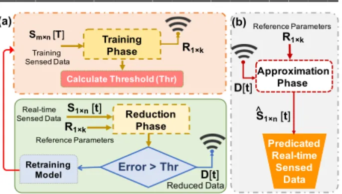
Fig. 1 shows general structure of the proposed adaptive threshold for multivariate data reduction models. It consists of three crucial phases including training phase, reduction phase at sensor board level and approximation stage at the sink level.
A.
Estimate Reference parameters / Approximation data
In this paper, the models based on PCA /MLR are mentioned because the proposed threshold has the potential to benefit different versions of PCA / MLR. However, for more clarity in this part, there are a few particulars versions of PCA and MLR will be discussed in this study. Due to limited resources of the sensor board, a lightweight version of PCA model called CCIPCA was used. It is explained in detail in [12], together with the steps of using CCIPCA in WSN as described in [11]. Furthermore, only 50 samples (training data) from 5000 samples used in this study for both models which is actually too small compared to training data have used in [11], where was about 700samples (training data) from 1000 samples used.
Estimate approximation data / Reference parameters (PCA-based)
1) Standardises the training data!̅#$%[']. 2) Implements CCIPCA
(!̅#$%[']) and estimates the eigenvector matrix )%×%. Then, reduces
the eigenvector matrix to +,-×.. )/0×% which is the reference
parameters is produced. It is then saved at the sensor node and transmit one copy of the parameter to the sink. 3) Standardises the new real-time sensed data S23×4[t] , then reduces it before transmitting by applying Eq. (1).
63×70[8] = S23×4[t] × )/0×% (1)
4) Sends the reduced data :;×<-[=] to the sink.5) Estimates the
approximation data at the senor node / sink by applying Eq. (2). S>3×4[t] = 63×70[8] × )/0×% (2) Fig.1. General structure of multivariate data reduction model with adaptive threshold: (a) sensor board level and (b) CH/BS Level.
Real-time Sensed Data Training Phase Reduction Phase Sm×n[T] Training Sensed Data Reduced Data (a) Reference Parameters Reference Parameters Retraining Model Calculate Threshold (Thr) R1×k S1×n[t] R1×k D[t] Error > Thr (b) D[t] R1×k S1×n[t] ^ Predicated Real-time Sensed Data Approximation Phase
Article #
————————————————————————————————————–
Estimate approximation data / Reference parameters (MLR-based)
1) After carefully studied the correlation between the multiple sensors on the same sensor board, the independence sensor ?@ and dependence sensor ?A are selected. Ambient temperature is selected as dependence
sensor ?A because it has the highest correlation with the surface
temperature and relative humidity. 2) Calculates the reference parameters by applying Eq. (3) and Eq. (4). where !̅@ , !̅A are the
average values for the variables !@ and !A ,respectively. In training
phase, ∀ !@ , !A∈ )3×# , F ≠ ℎ, ℎ IJK?8LK8 LKM F = 1,2. . , K. ℎ =
1 is the sensor index in the sensed data row S3×4[t]
Q@,3=
∑ZV[\STU,VWT̅UXSTU,VWT̅YX
∑ZV[\STU,VWT̅UX]
(3)
Q@,^= !̅@− (Q@3× !̅A) (4)
Thus reference parameters are generated as )(%W3)×b= [Q@,^ Q@,3] ,
F ≠ ℎ , F = 1,2. . , K . 3) Saves reference parameters in sensor boards and sends a copy of parameters to the sink. 4) Then, sends the reduced data cd to the sink.5) Estimates the approximation data at senor node
/ sink by applying Eq. (5) ∀ ?@, Q@,^, Q@,3, ?A ∈ )3×3 , F ≠
ℎ, ℎ IJK?8LK8
?@= Q@,^+ Q@,3× ?A (5)
B.
Estimate the Threshold Value in Training Phase
Steps for calculating the proposed threshold are described in the following Pseudo Code.
// Threshold estimation in Training Phase//
1 Input: Training data !#$%['], where n is the number of sensors and m is the number of collected samples in a specific period of time [T]. 2 Estimates the reference parameters where +;×f // k is the number
of reference parameters.
3 Calculates the relative error between the training data Sg×4[T] and
approximated data Sig×4[T] which is defined in Eq. (6).
jk×l[m] =n o
ip×q[r]Wop×q[r]n
op×q[r] l = ;, s. . .; k = ;, s … , v (6)
4 Estimates Threshold (Thr) by selecting maximum relative error value for all sensors of the same board. mdw ← yz{|jv×.[m]| //
C.
Update model during Reduction phase
In this phase, the real-time sensed data is reduced by applying the multivariate data reduction model. The model should update its reference when the relative error is larger than the threshold value which has been estimated in the training phase. Additionally, the threshold value is adjusted during retraining/updating phase based on new reference parameters. In evaluating, the algorithm includes a counter C to account for the frequency of the model re-training. The following pseudo code describes the updating stage of the model.
//Update model in Reduction Phase// 1) Reads new real-time sensed data S3×4[t] at current time t 2)
Calculates the approximated data Si3×4[t] by applying the reduction
model with its reference parameters )3×}3)Determines the model
error at current time [t] as stated in Eq. (7) j;×l[=] =n oi;×q[~]Wo;×q[~]n
o;×q[~] l = ;, s. . . (7)
4 If yz{|j;×.[=]| > Thr, then Update model; C=C+1;
5 Calculates the Threshold (Thr) // Call Training phase 6 ELSE: Sends the reduced data; End If Go to Step 1
D.
Approximation Phase
1)Receives new reduced data at current time t 2) Estimates the approximation data at sensor node / Sink by applying Eq. (2) for PCA-based model / Eq. (5) for MLR-based model.
Note:1) The approximation data at the sensor board is determined to calculate the model relative approximation error. 2) The approximation data at the sink is determined to reconstruct the original data.
V.
Performance Evaluation
In this paper, the multivariate data reduction models of PCA and MLR were applied to evaluate the proposed threshold and new performance metric. MATLAB software was used to simulate the data reduction models with adaptive and non-adaptive threshold using a real-time dataset called Lausanne Urban Canopy Experiment dataset (LUCE) [13]. LUCE is classified as a dynamic dataset and it includes ambient temperature, surface temperature and relative humidity.
A.
Numerical analysis for different multivariate data
reduction models with fixed buffer size
A sensor board with multiple sensors transmitted N=50000 samples during a time interval. The sensor board applied PCA and MLR models separately for each interval where the reduction ratio R% for PCA -1PC, PCA -2PC and MLR are 67%, 33% and 67% respectively. The model updated its reference parameters when the buffer size was set as W = {50 and 100}, n=3, EÄÅÇÉ= 52.92Üá, àâ@ä= EÄÅÇÉ/8,
!ç= K × 32 èF8? and !ê is 12 bytes , 24 bytes and 16 bytes for PCA
-1PC, PCA -2PC and MLR ,respectively .Where the number of parameters for MLR is 4, and the number of reference parameters for PCA is 3 in case of 1PC and 6 in case 2PC. Table 2 shows list of symbols used. The total energy consumption during a specific period is defined in Eqn. (8).
ë = (àê× Kê) + (àí × Kí), Kê= ì − Kí (8)
àê= (!ç× R%) × àâ@ä (9)
àí= ( (!ç× R%) + (!ê × 8)) × àâ@ä (10)
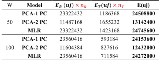
Table 1 shows the results of applying Eq. (8) for the above example. From the results, it is clear that the increment of the frequency of retraining/updating will negatively affect the energy consumption of the sensor board. It is because the size of the transmitted data after updating the model reference parameters is larger or equal to the payload data size without any reduction as defined in Eq. (10) and Eq. (9), which means that the edge device requires more energy in the transmission phase than the reduction stage. In this scenario (fixed window), UFM value is equal to (N / W). Thus, the UFM were 1000 and 500 for W=50 and W=100 respectively. The UFM can be reduced by selecting large value of W. But it is not a feasible solution due to the limited resource of the node.
Table 1. Comparison Energy consumption
B. Results and Discussion
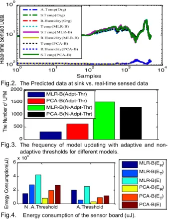
Fig. 2, Fig. 3 and Fig. 4 show the results of simulation for the PCA and MLR models with adaptive and non-adaptive threshold. It is clear
W Model j+ (ñk)× Kê jm(ñk)× Kí E(uj) 50 PCA-1 PC 23322432 1186368 24508800 PCA-2 PC 11487168 1655232 13142400 MLR 23322432 1423168 24745600 100 PCA-1 PC 23560416 593184 24153600 PCA-2 PC 11604384 827616 12432000 MLR 23560416 711584 24272000
Article #
————————————————————————————————————–
Page 4 of 4 that the adaptive threshold has managed to reduce the frequency of model updating its reference parameters by 80% and 52% which is better than the one with non- adaptive threshold for multivariate data reduction models MLR-B and PCA-B respectively. The power consumption of the model by applying adaptive threshold is found to be less than the non-adaptive threshold. Based on the results, it is concluded that frequency of model updating is crucial in evaluating the multivariate data reduction models.
VI. CONCLUSIONS AND FUTURE WORK
Results show that the proposed metric validates its effectiveness in the performance of multivariate data reduction models in terms of the sensor node energy consumption. The adaptive threshold improves the frequency of updating the parameters by 80% and 52% in comparison to the non-adaptive threshold for multivariate data reduction models of MLR-B and PCA-B respectively. The proposed metric and threshold were tested using the environmental data. This study is recommended to be the future work test for the same model that employs multivariate vibration data.Fig.2. The Predicted data at sink vs. real-time sensed data
Fig.3. The frequency of model updating with adaptive and non-adaptive thresholds for different models.
Fig.4. Energy consumption of the sensor board (uJ). Table 2. List of symbols used
Symbols Description
Kê, Kí the number of message transmissions in the reduction phase the number of UFM
!ç,!) the size of the original sensed data and of model reference parameters
R% the model data reduction ratio
àê,àí the cost of energy consumption for transmission of data in the reduction phase and retraining phase, respectively.
E the total energy consumption during a specific period.
EÄÅÇÉ, àâ@ä the energy consumption per Byte and bits, respectively.
óò the number of Principal Components (PC) for PCA
ACKNOWLEDGEMENT
This research is supported by the Fundamental Research Grant Scheme (FRGS) vote number 1532 from the Ministry of Education Malaysia.
REFERENCES
[1] Y. Zhang, N. Meratnia, P. Havinga, “Outlier detection techniques for wireless sensor networks: A survey. IEEE Comm. Surveys & Tutorials. 1;12(2):159-70, 2010. [2] M. A. Rassam, A. Zainal, and M. A. Maarof, “Advancements of data anomaly
detection research in Wireless Sensor Networks: A survey and open issues,” Sensors, vol. 13, no. 8, pp. 10087–10122, 2013.
[3] Alduais, N. A. M., J. Abdullah, A. Jamil, and L. Audah. "An efficient data collection and dissemination for IOT based WSN." In IEEE Information Technology, Electronics and Mobile Communication Conference (IEMCON), pp. 1-6, 2016. [4] K. A. Bispo, et al., “A semantic solution for saving energy in wireless sensor
networks,” Proc. - IEEE Symp. Comput. Commun., pp. 000492–000499, 2012. [5] L. Tan and M. Wu, “Data reduction in wireless sensor networks: a hierarchical LMS
prediction approach,” IEEE Sensors J., no. c, pp. 1–1, 2015.
[6] F. Strakosch and F. Derbel, Fast and Efficient Dual-Forecasting Algorithm for Wireless Sensor Networks, Nuremberg, Germany: Proceedings of the SENSOR 2015 (pages 859–863), 2015.
[7] Arbi, Imen Ben, F. Derbel, and F. Strakosch. "Forecasting methods to reduce energy consumption in WSN." In IEEE Inst. Meas. Tech. Conf. (I2MTC), pp. 1-6, 2017. [8] C. Carvalho, D. G. Gomes, N. Agoulmine, and J. N. de Souza, “Improving prediction
accuracy for WSN data reduction by applying multivariate spatio-temporal correlation,” Sensors, vol. 11, no. 11, pp. 10010–10037, 2011.
[9] M. A. Rassam and A. Zainal, “Principal Component Analysis-Based Data Reduction Model for Wireless Sensor Networks,” Int. J. Ad Hoc Ubiquitous Comput., vol. 18, no. 1–2, pp. 85–101, 2015.
[10] U. Jaimini, et al., “Investigation of an Indoor Air Quality Sensor for Asthma Management in Children,” IEEE Sensors Letters., vol. 1, no. 2, pp. 1–1, 2017. [11] M. A. Rassam, A. Zainal, and M. A. Maarof, “An adaptive and efficient dimension
reduction model for multivariate wireless sensor networks applications,” Appl. Soft Comput., vol. 13, no. 4, pp. 1978–1996, 2013.
[12] J. Weng, Y. Zhang, and W.-S. Hwang, “Candid Covariance-Free Incremental Principal Component Analysis,” IEEE Trans. Pattern Anal. Mach. Intell., vol. 25, no. 8, pp. 1034–1040, 2003.
[13] “LUCE,” Lausanne Urban Canopy Experiment (LUCE), 2007. [Online]. Available: http://lcav.epfl.ch/cms/lang/en/ pid/86035.
100 101 102 103 104 100 101 102 R ea l-t im e S en se d D at a Samples A.T emp(Org) S.T emp(Org) R.Humidit y(Org) T emp(MLR-B) S.T emp(MLR-B) R.Humidit y(MLR-B) T emp(PCA-B) R.Humidit y(PCA-B) S.T emp(PCA-B) 0 500 1000 1500 2000 Th e N um be r of U FM MLR-B(Adpt-Thr) PCA-B(Adpt-Thr) MLR-B(N-Adpt-Thr) PCA-B(N-Adpt-Thr) N .A.Threshold A.Threshold 0 2 4 6x 10 6 En re gy C on su m pt io n( uJ ) MLR-B(E R) MLR-B(E T) MLR-B(E) PCA-B(ER) PCA-B(ET) PCA-B(E)