INAUGURAL - DISSERTATION
zur
Erlangung der Doktorwürde der Naturwissenschaftlich-Mathematischen Gesamtfakultät der Ruprecht-Karls-Universität Heidelberg vorgelegt von
Diplom-Mathematiker mit Ausrichtung Wissenschaftliches Rechnen und Diplom-Volkswirt
Jan Christoph Neddermeyer
aus Darmstadt
Importance Sampling-Based Monte Carlo Methods
with Applications to Quantitative Finance
Gutachter: Prof. Dr. Rainer Dahlhaus Prof. Dr. Dieter W. Heermann
Abstract
In the present work advanced Monte Carlo methods for discrete-time stochastic processes are developed and investigated. A particular focus is on sequential Monte Carlo methods (particle filters and particle smoothers) which allow the estimation of nonlinear, non-Gaussian state-space models. The key technique which underlies the proposed algorithms is importance sampling. Computationally efficient nonparametric variants of importance sampling which are generally applicable are developed. Asymptotic properties of these methods are analyzed theoretically and it is shown empirically that they improve over existing methods for relevant applications. Particularly, it is shown that they can be applied for financial derivative pricing which constitutes a high-dimensional integration problem and that they can be used to improve sequential Monte Carlo methods.
Original models in general state-space form for two important applications are proposed and new sequential Monte Carlo algorithms for their estimation are developed. The first application concerns the on-line estimation of the spot cross-volatility for ultra high-frequency financial data. This is a challenging problem because of the presence of microstructure noise and non-synchronous trading. For the first time state-space models with non-non-synchronously evolving states and observations are discussed and a particle filter which can cope with these models is designed. In addition, a new sequential variant of the EM algorithm for parameter estimation is proposed. The second application is a non-linear model for time series with an oscillatory pattern and a phase process in the background. This model can be applied, for instance, to noisy quasi-periodic oscillators occurring in physics and other fields. The estimation of the model is based on an advanced particle smoother and a new nonparametric EM algorithm.
The dissertation is accompanied by object-oriented C++ implementations of all proposed
Zusammenfassung
In der vorliegenden Arbeit werden fortgeschrittene Monte-Carlo-Verfahren für zeitdiskrete stoch-astische Prozesse entwickelt und untersucht. Ein Schwerpunkt wird dabei auf sequentielle Monte-Carlo-Verfahren (Partikel-Filter und Partikel-Smoother) gesetzt; diese werden zur Schätzung von nichtlinearen, nicht-Gauß’schen State-Space-Modellen verwendet. Importance Sampling ist die Schlüsselmethode, auf der die entwickelten Algorithmen basieren. Es werden nichtparametrische Varianten des Importance Samplings entwickelt, die recheneffizient und allgemein anwendbar sind. Asymptotische Eigenschaften dieser Methoden werden theoretisch untersucht und es wird anhand relevanter Anwendungen gezeigt, dass sie bessere Ergebnisse liefern als existierende Ver-fahren. Insbesondere wird gezeigt, dass sie für die Bewertung von Finanzderivaten, ein hochdi-mensionales Integrationsproblem, verwendet werden können und dass sie benutzt werden können um sequentielle Monte-Carlo-Verfahren zu verbessern.
Für zwei wichtige Anwendungen werden neue Modelle in State-Space-Form entwickelt und sequentielle Monte-Carlo-Algorithmen beschrieben, die für deren Schätzung genutzt werden kön-nen. Die erste Anwendung betrifft die Online-Schätzung der Spot Kreuz-Volatilität für ultra-hochfrequente Finanzdaten. Aufgrund des Mikrostruktur-Rauschens und der nicht-synchronen Handelszeitpunkte stellt dies ein schwieriges Problem dar. Im Zuge dieser Anwendung werden erstmals State-Space Modelle mit nicht-synchronen Zuständen und Beobachtungen betrachtet und ein Partikel-Filter konstruiert, der für solche Modelle geeignet ist. Außerdem wird ein neuartiger sequentieller EM-Algorithmus für die Parameter-Schätzung entwickelt. Als zweite An-wendung wird ein nichtlineares Modell für Zeitreihen vorgeschlagen, die ein periodisches Muster und einen latenten Phasen-Prozess aufweisen. Dieses Modell kann u.a. verwendet werden um verrauschte quasi-periodische Oszillatoren zu beschreiben, die in verschiedenen Disziplinen (z.B. der Physik) vorkommen. Die Schätzung dieses Modells basiert auf einem erweiterten Partikel-Smoother und einem neuen nichtparametrischen EM-Algorithmus.
Teil dieser Dissertation sind außerdem objektorientierte C++-Implementierungen aller
vor-geschlagenen Algorithmen, die besonders auf die Wiederverwendbarkeit und Erweiterbarkeit Wert legen.
Acknowledgements
I extend my thanks to my supervisor Prof. Dr. Rainer Dahlhaus and my co-supervisor Prof. Dr. Dieter W. Heermann for giving me the opportunity to work on this exciting topic. Particularly, I like to thank Prof. Dr. Rainer Dahlhaus for his invaluable support in terms of scientific advice and hardware/software equipment. I would also like to express my gratitude to Dr. Cornelia Wichelhaus, Prof. Dr. Jan Johannes, Konstantinos Paraschakis, Dr. Markus Fischer, and Julian Kunkel for very useful comments and inspiring discussions at different stages of this project. Similarly, my gratitude goes Dr. Ulrich Brandt-Pollmann who made possible my three month stay in London. Finally, I want to thank my wife Paula and the rest of my family for their continuing support.
This work was supported by the Deutsche Forschungsgemeinschaft under DA 187/15-1 and by the University of Heidelberg under Frontier D.801000/08.023. In addition, I am grateful to Heidelberg Graduate School of Mathematical and Computational Methods for the Sciences for funding my travels to various conferences and workshops.
Contents
Abbreviations v
1 Introduction 1
1.1 Overview of the Problems, Methods, and Applications . . . 1
1.2 Outline of the Results . . . 3
2 Monte Carlo Methods and General State-Space Models 7 2.1 Monte Carlo Approximation . . . 7
2.2 Computational Efficiency and Variance Reduction Techniques . . . 8
2.3 Importance Sampling . . . 8
2.4 General State-Space Models and Sequential Monte Carlo . . . 10
2.5 Expectation-Maximization Algorithm . . . 14
2.6 Pseudo- and Quasi-Random Number Generation . . . 14
3 Nonparametric Importance Sampling 17 3.1 Introduction . . . 17
3.2 A New Nonparametric Importance Sampling Algorithm . . . 18
3.3 A New Nonparametric Self-Normalized Importance Sampling Algorithm . . . 22
3.4 Applying Nonparametric Importance Sampling . . . 23
3.4.1 Parameter Selection . . . 24
3.4.2 Implementing the LBFP Estimator . . . 24
3.4.3 Computational Remarks . . . 26
3.5 Simulations . . . 26
3.6 Application: Spam Filter . . . 32
4 Nonparametric Partial Importance Sampling for Financial Derivative Pricing 37 4.1 Introduction . . . 37
4.2 Derivative Pricing and Importance Sampling . . . 38
4.3 Nonparametric Partial Importance Sampling . . . 39
4.4 Effective Dimension . . . 41
4.5 Gaussian Models . . . 42
4.7 Comparison with Parametric Importance Sampling . . . 44
4.8 Implementation of the Algorithm . . . 45
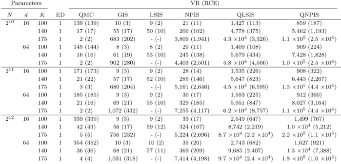
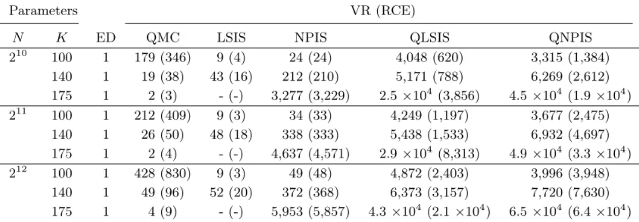
4.9 Simulation Results . . . 47
5 Nonparametric Particle Filtering and Smoothing 57 5.1 Introduction . . . 57
5.2 A Nonparametric Particle Filter . . . 58
5.3 A Nonparametric Particle Smoother . . . 60
5.4 On-Line Maximum Likelihood Parameter Estimation . . . 61
5.5 Quasi-Monte Carlo Sampling . . . 64
5.6 Bin Width Selection . . . 64
5.7 Simulations . . . 66
5.7.1 Benchmark Model . . . 67
5.7.2 High-Frequency Stochastic Volatility Application . . . 70
6 Particle Filter-Based On-Line Estimation of Spot Cross-Volatility 75 6.1 Introduction . . . 75
6.2 A New Nonlinear Market Microstructure Noise Model . . . 77
6.3 On-Line Estimation of Spot Volatility Based on a Particle Filter and Sequential EM-Type Algorithms . . . 81
6.3.1 A Nonlinear State-Space Model . . . 81
6.3.2 An Efficient Particle Filter . . . 82
6.3.3 Sequential EM-Type Algorithms . . . 84
6.3.4 Summary . . . 87
6.4 From Transaction Time to Clock Time . . . 89
6.4.1 Clock Time Spot Volatility Estimation . . . 89
6.4.2 An Alternative Estimator for Clock Time Spot Volatility . . . 89
6.5 Fine-Tuning of the Volatility Estimator in the Time-Varying Case . . . 91
6.5.1 Adaptive Step Size Selection . . . 91
6.5.2 On-line Bias Correction and Mean Squared Error Minimization . . . 92
6.6 Spot Cross-Volatility Estimation: New Modeling Aspects . . . 97
6.6.1 A New Transaction Time Model for Non-Synchronous Data . . . 97
6.6.2 Non-Standard State-Space Models for Non-Synchronous Data . . . 98
6.7 On-Line Estimation of Spot Cross-Volatility . . . 99
6.7.1 A State-Space Model with Non-Synchronous Observations and States . . . 99
6.7.2 An Original Particle Filter for Non-Synchronous State-Space Models . . . 100
6.7.3 EM-Type Algorithms for Non-Synchronous Observations and States . . . 103
6.8 Clock Time Covariance Estimation . . . 105
6.9 Implementation Details . . . 106
6.10 Simulations and Applications . . . 109
CONTENTS
6.10.2 Results for Real Data . . . 114
6.11 Discussion . . . 118
7 Bayesian Phase Estimation for Noisy Quasi-Periodic Time Series 123 7.1 Introduction . . . 123
7.2 A New State-Space Model for Quasi-Periodic Time Series . . . 124
7.3 The Estimation Method . . . 125
7.3.1 Rao-Blackwellized Particle Filtering . . . 125
7.3.2 Rao-Blackwellized Fixed-Lag Particle Smoothing . . . 127
7.3.3 A Stochastic EM Algorithm for Parameter Estimation . . . 128
7.4 Nonparametric Estimation of the Fluctuation Pattern . . . 129
7.5 Discussion . . . 131
7.6 Simulations . . . 132
7.6.1 Simulated Data . . . 132
7.6.2 Noisy Rössler Attractor . . . 135
7.6.3 Application to Human Electrocardiogram Recordings . . . 139
8 Software 141 8.1 Overview . . . 141
8.2 Main Software Packages . . . 141
8.3 Auxiliary Libraries . . . 143
Conclusions and Prospects 144 Appendix A Proofs 149 A.1 Proof of Theorem 3.1 . . . 149
A.2 Lemma A.1 . . . 152
A.3 Lemma A.2 . . . 153
A.4 Proof of Theorem 3.3 . . . 153
A.5 Proof of Theorem 3.4 . . . 155
A.6 Derivation of the complexity of the LBFP . . . 156
A.7 Proof of Theorem 4.1 . . . 156
A.8 Proof of Proposition 5.1 . . . 157
A.9 Proof of Proposition 6.1 . . . 159
A.10 Calculation of the Quasi Mean Squared Error in Section 6.5.2 . . . 159
A.11 Reversed Order Initialization . . . 160
A.12 Proof of Proposition 7.1 . . . 161
A.13 Proof of Proposition 7.2 . . . 162
Abbreviations
APF Auxiliary particle filter
BSPS Backward simulation particle smoother CDIS Change-of-drift importance sampling CV Coefficient of variation
ED Effective dimension
GSSM General state-space model
IS Importance sampling
LBFP Linear blend frequency polygon LSIS Least-squares importance sampling
MC Monte Carlo
NPIS Nonparametric partial importance sampling NIS Nonparametric importance sampling
NPF Nonparametric particle filter NPS Nonparametric particle smoother
NSIS Nonparametric self-normalized importance sampling PCA Principal component analysis
QMC Quasi-Monte Carlo
RBPS Rao-Blackwellized particle smoother RCE Relative computational efficiency RE Relative efficiency
RMSE Root mean square error
SIRMH Bootstrap particle filter with Metropolis-Hastings moves SCVE Spot cross-volatility estimation
SPS Simple particle smoother SVE Spot volatility estimation
Chapter 1
Introduction
1.1
Overview of the Problems, Methods, and Applications
The simulation of stochastic processes and the approximation of complex, high-dimensional in-tegrals which depend on stochastic processes are frequent problems in many fields. Numerical integration schemes are often infeasible as a result of the curse of dimensionality and computa-tional limitations. Monte Carlo simulation is frequently the only tractable method because its convergence rate is independent of the problem dimension. However, if the problem dimension is large or the integrand very irregular crude Monte Carlo is inefficient. This establishes a need for advanced Monte Carlo algorithms. In the last decades, advanced Monte Carlo methods became more and more relevant for practical applications as a result of increasing computing power. In particular, in Bayesian inference Monte Carlo methods such as Markov Chain Monte Carlo and sequential Monte Carlo methods experienced a distinct surge in popularity.
In this dissertation, the main focus is on sequential, discrete-time models and methods. Discrete-time models occur, for instance, as discretizations of continuous-time stochastic pro-cesses. The on-line or sequential estimation which is frequently required when dealing with stochastic processes is of key focus in this work. However, off-line settings are also considered. New Monte Carlo methods are proposed and analyzed concerning both theoretical and computa-tional aspects. Efficient software implementations of the algorithms are provided. The usefulness of the proposed methods is verified through relevant applications. Several complex applications in the field of quantitative finance are considered in detail.
The technique which constitutes the fundamental concept of the methods developed in this dissertation is importance sampling. This is a very flexible sampling method which can be used to generate random samples from intractable distributions or to reduce the Monte Carlo vari-ance. It is frequently applied to rare event simulation. A typical application is the computation of rare event probabilities. Already in the 1950s, importance sampling were used in rare event applications in physics (Kahn 1950; Kahn and Marshall 1953). However, importance sampling is much more powerful and by far not limited to the simulation of rare events. Generally speaking, almost any Monte Carlo approximation can be improved significantly through the use of impor-tance sampling. The basic idea of imporimpor-tance sampling is to generate samples from an auxiliary
distribution which is known as proposal instead of from the target distribution. Subsequently, the samples are weighted such that they approximate the target distribution. The main difficulty of applying importance sampling in practice is the choice of a suitable proposal. This issue is tackled in this work.
Most existing importance sampling methods are based on a parametric choice of the pro-posal, that is the proposal is chosen from a parametrized family of distributions. In addition, nonparametric importance sampling methods have been developed. They are based on non-parametric approximations of the (optimal) proposal. Until now, nonnon-parametric importance sampling was merely a nice theoretical alternative to parametric importance sampling with no practical applications. The reason for this in founded in the computational inefficiency of existing nonparametric importance sampling techniques. In this dissertation, computationally efficient nonparametric importance sampling algorithms which are suitable for practical application are proposed and investigated.
A relevant application where (nonparametric) importance sampling can be effectively applied is the pricing of path-dependent financial derivatives. There, Monte Carlo approximations of complex high-dimensional integrals are required. In addition, the computational efficiency of the method used is important because the evaluation of financial derivative prices is often time-critical. Although parametric importance sampling methods already belong to the standard toolbox in financial engineering, nonparametric importance sampling techniques have not been applied until now. The evolution of a financial asset can be described through a stochastic differential equation with a Brownian motion as driving process. Based on this model the price of a European option can be approximated through a high-dimensional integral which depends on a discretization of the stochastic differential equation. It is shown that the proposed nonparametric importance sampling algorithms lead to massive efficiency gains for such kind of integration problems.
In this work, particle filters and particle smoothers which belong to the class of sequential Monte Carlo methods are of particular interest. Sequential Monte Carlo methods are Bayesian simulation techniques that allow the approximation of the filtering and smoothing distributions of general state-space models. Numerous applications which comply with the class of general state-space models are readily available, for instance object tracking problems in engineering and stochastic volatility estimation in finance. General state-space models often occur naturally as discretizations of stochastic differential equations with hidden components. In contrast to the traditional linear state-space models, general state-space models allow for nonlinear functions and non-Gaussian noise distributions. Consequently, standard methods for filtering and smoothing in (linear) state-space models such as the Kalman filter and the Kalman smoother can usually not be applied.
An essential ingredient of the sequential Monte Carlo methods considered here is importance sampling. It is required because direct sampling from the target distribution is impossible. A goal is to develop more efficient particle filters and smoothers by employing nonparametric importance sampling schemes and quasi-Monte Carlo techniques.
1.2. OUTLINE OF THE RESULTS
Carlo methods, which are of great importance, are considered in detail. Both are hot topics in their areas of research. The methods and models proposed in this work are original contributions and they have not been used for these applications before. The first application is the on-line estimation of spot cross-volatility for ultra high-frequency financial data. The spot cross-volatility is the key quantity in risk management, portfolio optimization, and trading. The main problems are the presence of so-called market microstructure noise and the non-synchronous trading times of different securities. Particularly for the non-synchronous trading times there is a lack of appropriate models. Our approach is different from existing approaches and it includes several new modeling and estimation aspects. It is shown, in particular, that ultra high-frequency financial data can be effectively treated in a nonlinear state-space framework.
The second application concerns the estimation of a general time series model which is also newly proposed. It is a model for stationary time series with a specific oscillatory component which can be written in state-space form. This model includes quasi-periodic oscillators with a latent phase process in the background. Our approach is very general and allows the model-ing and estimation of nonlinear phase transitions, time-varymodel-ing amplitudes, baseline shifts, and general oscillatory patterns. In particular, the estimation of the phase is of interest because it is, for instance, required for the analysis of phase synchronization of coupled oscillators. Many applications complying with our model exist in different fields such as physics, engineering, and neuroscience. An interesting example which is briefly considered in this dissertation are elec-trocardiogram (ECG) recordings measuring the electrical activity of the heart over time. For ECG data existing methods for phase estimation such as the Hilbert transform are inappropriate because of baseline shifts and a non-trigonometric oscillatory pattern which are present in the data. Our method not only allows inference on the phase but also the nonparametric estimation of the characteristic oscillatory pattern.
1.2
Outline of the Results
The results of this dissertation are presented in several research papers which are already pub-lished or available as preprints. The following description summarizes the major contributions of this work and indicates the corresponding research papers. Chapter 2 gives a literature review which provides the foundation of the present work. Chapter 8 overviews the software packages which were developed.
Chapter 3 (Neddermeyer 2009)
The variance reduction established by importance sampling strongly depends on the choice of the importance sampling distribution. A good choice is often hard to achieve especially for high-dimensional integration problems. It is shown that nonparametric estimation of the optimal importance sampling distribution (known as nonparametric importance sampling) is a reasonable alternative to parametric approaches. New nonparametric variants of both the self-normalized and the unnormalized importance sampling estimator are proposed and investigated. A common critique on nonparametric importance sampling is the increased
computational burden compared with parametric methods. This problem is solved to a large degree by utilizing the linear blend frequency polygon estimator instead of a kernel estimator. Mean square error convergence properties are investigated theoretically leading to recommendations for the efficient application of nonparametric importance sampling. Particularly, it is shown that nonparametric importance sampling asymptotically attains optimal importance sampling variance. As an application, the estimation of the distribution of the queue length of a spam filter queueing system based on real data is considered.
Chapter 4 (Neddermeyer 2010a)
It is shown how nonparametric importance sampling can be effectively used for financial derivative pricing. Standard nonparametric importance sampling is inefficient for this task because the approximation of high-dimensional integrals are required. This issue is solved by applying the procedure to a low-dimensional subspace, which is identified through principal component analysis and the concept of the effective dimension. This leads to the method of nonparametric partial importance sampling. The mean square error properties of the algorithm are investigated and its asymptotic optimality is shown. Quasi-Monte Carlo is used for further improvement of the method. It is demonstrated through path-dependent and multi-asset option pricing problems that the algorithm leads to significant efficiency gains compared with existing methods.
Chapter 5 (Neddermeyer 2010b)
An original particle filter and an original particle smoother which employ nonparametric importance sampling are developed. It is shown that these algorithms provide a better approximation of the filtering and smoothing distributions than standard methods. The methods’ advantage is most distinct in severely nonlinear situations. In contrast to most existing methods, they allow the use of quasi-Monte Carlo sampling. In addition, they do not suffer from weight degeneration rendering unnecessary a resampling step. For the estimation of model parameters an efficient on-line maximum likelihood estimation technique is proposed which is also based on nonparametric approximations. All suggested algorithms have almost linear complexity for low-dimensional state-spaces. This is an advantage over standard smoothing and maximum likelihood procedures. Particularly, all existing sequential Monte Carlo methods that incorporate quasi-Monte Carlo sampling have quadratic complexity. As an application, stochastic volatility estimation for high-frequency financial data is considered, which is of great importance in practice.
Chapter 6 (Dahlhaus and Neddermeyer 2010a, b)
We develop a new technique for the on-line estimation of both constant and time-varying spot covariance matrices (spot cross-volatilities) in the presence of market mi-crostructure noise. The algorithm works directly on the non-synchronous transaction data and updates the covariance estimate immediately after the occurrence of a new transaction. The transaction prices are considered as noisy observations of latent efficient log-price pro-cesses. A new transaction time model for the efficient log-prices is proposed which models
1.2. OUTLINE OF THE RESULTS
the evolution of different securities in individual transaction times. In addition, a new non-linear market microstructure noise model is developed which reproduces the major stylized facts of high-frequency data such as the price discreteness and the negative first-order au-tocorrelation of the returns. Our model takes the form of a nonlinear state-space model with non-synchronous states and observations. Based on this representation a new particle filter is designed that allows the approximation of the filtering distributions of the efficient log-prices. It is shown that the spot covariance matrix of the latent log-price processes can be estimated as a parameter of the state-space model. For this purpose we propose a sequential variant of the EM algorithm that uses the output of the particle filter. For the univariate case we also propose an on-line bias correction and a method for adaptive step size selection. The practical usefulness of our technique is verified through Monte Carlo simulations and through an application to real transaction data.
Chapter 7 (Dahlhaus and Neddermeyer 2009)
We introduce a new model for stationary time series with a quasi-periodic component. The aim is to model time series with a specific fluctuation pattern and an unobserved phase process in the background. The model also includes a time-varying amplitude and baseline. This allows the modeling of data occurring in physics, biology, life science, and many other fields. The goals are to estimate the unobserved phase, amplitude, and baseline processes as well as the fluctuation pattern. The model can be written as a nonlinear, non-Gaussian state-space model treating the phase, the amplitude, and the baseline as latent Markov pro-cesses. For the estimation, we suggest a Rao-Blackwellized particle smoother that combines the Kalman smoother and an efficient sequential Monte Carlo smoother. For the estima-tion of the fluctuaestima-tion pattern, an original nonparametric EM algorithm is developed. The proposed algorithms can be applied on-line, they are easy to implement and computation-ally efficient. The method’s potential for practical applications is demonstrated through simulations and an application to human electrocardiogram recordings.
Chapter 2
Monte Carlo Methods and General
State-Space Models
This chapter introduces notation and provides a brief overview of major concepts of Monte Carlo simulation which are relevant for the methods developed in the following chapters.
2.1
Monte Carlo Approximation
Monte Carlo simulation can be used to approximate a probability density function p on Rd or
the expectation
Ep[ϕ] =Iϕ=
Z
ϕ(x)p(x)dx
of some function ϕ:Rd → R with respect to p. Let’s assume N i.i.d. samples {xi}Ni=1 from p are available. Then, an empirical estimate of densityp is given by
p(x)≈ 1 N N X i=1 δxi(x)
withδ being the Dirac delta function. The integral Iϕ can be estimated through
ˆ IϕMC= 1 N N X i=1 ϕ(xi). (2.1) Clearly, IˆMC
ϕ is a consistent, unbiased estimator of Iϕ. If the varianceσ2 =Var[ϕ]is finite then
the standard central limit theorem gives
√
N( ˆIϕMC−Iϕ)⇒ N(0, σ2).
The central limit theorem implies that the convergence rate of (standard) Monte Carlo integration is independent of the dimension of the integrand. This constitutes a major advantage of Monte Carlo simulation-based methods compared with numerical integration techniques.
In many applications, it is impossible or at least very difficult to generate i.i.d samples fromp.
This is often the case whenpis high-dimensional, not given in closed form, or as usual in Bayesian
settings when p is only known up to a constant. In Section 2.3, the concept of importance
sampling is described which allows the generation of weighted samples that approximate arbitrary probability density functions.
To reduce the (Monte Carlo) variance of the estimator (2.1) one can apply variance reduction techniques which are briefly considered in the following section.
2.2
Computational Efficiency and Variance Reduction Techniques
To make Monte Carlo algorithms comparable, it is useful to quantify the efficiency of a Monte Carlo estimator. Let’s assume X is a random variable defined on a probability space (Ω,B,P)and is used to estimate some quantity µ. The computational efficiency of the estimator X can
be defined through
CE[X] = (MSE[X]C[X])−1,
where MSE[X]denotes the mean square error ofX andC[X]the average costs of computing one
realization ofX(L’Ecuyer 1994). From this definition, one observes that efficiency improvements
can be achieved either by reducing the mean square error or the computational costs. The computational costs can be reduced through more efficient algorithms or a faster implementation. In particular, the random number generator used is a critical component because of its frequent use in Monte Carlo simulation (see Section 2.6).
Methods which are applied to reduce the mean square error MSE[X]are known as variance
reduction techniques. Relevant methods are importance sampling, antithetic sampling, moment matching, and control variates (Jäckel 2002; Glasserman 2004; Robert and Casella 2004). Most of these techniques aim at improving a given set of samples which is used for Monte Carlo integration. More precisely, the i.i.d. samples{xi}N
i=1 are transformed into non-i.i.d. samples in a way such that the mean square error of the estimator (for instanceIˆMC
ϕ in (2.1)) is reduced. In
contrast, importance sampling is based on a change of the distribution from which the samples are drawn. The Monte Carlo methods proposed in this dissertation are based on importance sampling. However, it is mentioned that most of the proposed methods could be (further) improved by the additional use of other variance reduction techniques.
2.3
Importance Sampling
Importance sampling is the fundamental concept underlying the Monte Carlo methods developed in this dissertation. It is a general sampling technique which can be used to approximate an integral Iϕ. It is often applied if direct sampling from the distribution p is computationally
too demanding or intractable. But it is not limited to this purpose. Unless ϕ is constant,
importance sampling can often yield a massive reduction of the estimator’s variance, if applied carefully. Formally, importance sampling is a change of measure. The expectation Ep[ϕ] is
2.3. IMPORTANCE SAMPLING
rewritten as
Eq[ϕw] =
Z
ϕ(x)w(x)q(x)dx,
whereq is the probability density function of an importance sampling distribution (also known
as proposal) andw(x) =p(x)/q(x) is the Radon-Nikodym derivative ofpwith respect toq. The
proposal needs to be chosen so that its support includes the support of|ϕ|por p, which imposes
a first constraint onq. Using importance sampling the integralIϕ can be estimated by
ˆ IϕIS= 1 N N X i=1 ϕ(xi)w(xi), (2.2)
where the samples{xi}N
i=1 are drawn from proposalq. Note,IˆϕISis an unbiased estimator of Iϕ.
In Bayesian inference, it is often the case that either p or the proposal q (or both) are
only known up to some constant. In this case an alternative is the self-normalized importance sampling estimator given by
ˆ IϕSIS= PN i=1ϕ(xi)w(xi) PN i=1w(xi) . (2.3) In contrast to IˆIS
ϕ, IˆϕSIS is biased. The strong law of large numbers implies that both IˆϕIS and
ˆ
IϕSIS converge almost surely to the expectation Iϕ if it is finite. However, this result is neither
of help for assessing the precision of the estimators for a finite set of samples nor for the rate of convergence. In order to construct error bounds, it is desirable to have a central limit theorem at hand. Under the assumptions thatIϕand Varq[ϕw]are finite, a central limit theorem guaranties
√
N( ˆIϕIS−Iϕ)⇒ N(0, σ2IS),
whereσIS2 =Eq[ϕw−Iϕ]2 (Rubinstein 1981). The proposal which minimizes the varianceσIS2 is
given by
qϕIS(x) = R |ϕ(x)|p(x)
|ϕ(x)|p(x)dx. (2.4)
qϕISis called the optimal proposal. Remarkably, the importance sampling estimator based on the
optimal proposal has zero variance for functions ϕ with a definite sign. However, the optimal
proposal is unavailable in practice because of its unknown denominator. A central limit theorem for the self-normalised importance sampling estimatorIˆSIS
ϕ can be established
√
N( ˆIϕSIS−Iϕ)⇒ N(0, σSIS2 ) (2.5) with limiting varianceσ2SIS=Eq[(ϕ−Iϕ)w]2 under the additional assumption that Varq[w]<∞
(Geweke 1989). The varianceσ2SIS is minimized by the proposal
qϕSIS(x) = R |ϕ(x)−Iϕ|p(x)
|ϕ(x)−Iϕ|p(x)dx
, (2.6)
provided that the median of ϕ with respect to p exists. The optimal proposals (2.4) and (2.6)
least as difficult as the original integration problem. In practice, the objective is to find an easy-to-sample density that approximates the optimal proposals. Traditionally, a proposal is chosen from some parametric family of densities{qϕ,θ;θ∈Θ}that satisfy the assumptions of the
central limit theorems or some related conditions. Typically, it is demanded that the support of
qϕ,θ includes the support of|ϕ|p or |ϕ−Iϕ|p, respectively, and that the tails of q do not decay
faster than those of |ϕ|p. Many different density classes have been investigated in the literature
including multivariate Student t, mixture, and exponential family distributions (see for instance Geweke 1989; Stadler and Roy 1993; Oh and Berger 1993). The parametrized choice of the proposal can be adaptively revised during the importance sampling which is known as adaptive importance sampling (Oh and Berger 1992; Kollman et al. 1999). Often expectationIϕ needs to
be computed for many different functionsϕleading to different optimal proposals. Consequently,
it is necessary to investigate the structure of any new ϕ in order to find a suitable parametric
family.
2.4
General State-Space Models and Sequential Monte Carlo
A general state-space model describes the joint evolution of a hidden state sequence and an observation sequence. The states Xt,t= 0,1, . . ., taking values in Rd constitute an unobservedMarkov process. The observations Yt, t = 1,2, . . ., which take values in Rs, are conditionally
independent given the states. A general state-space model is fully specified by the transition distributions and the observation distributions
Xt|Xt−1 ∼ p(xt|xt−1), (2.7)
Yt|Xt ∼ p(yt|xt). (2.8)
The initial stateX0is distributed according to some prior densityp(x0). Alternatively, a general state-space model can be specified through a state equation and an observation equation
Xt = ft(Xt−1, ηt), (2.9)
Yt = gt(Xt, t), (2.10)
where ft, gt are (nonlinear) functions and ηt, t are mutually and serially independent noise
variables.
Many stochastic processes with latent components occurring in engineering, physics, finance, and other fields have a natural (general) state-space representation (see Doucet, de Freitas, and Gordon 2001; Lin et al. 2005 and the references there). For instance, discretizations of stochastic differential equations often lead directly to state-space models. A state-space model has a nice representation in terms of a graphical model (see Figure 2.1) and it exhibits certain conditional independence properties which can be easily verified, for instance, p(yt|x0:t,y1:t−1) = p(yt|xt)
and p(xt|x0:t−1,y1:t−1) =p(xt|xt−1). Note, the notation y1:t={y1, . . . ,yt} is used throughout
this dissertation.
The objective is to compute the filtering distributions p(xt|y1:t) or smoothing distributions
2.4. GENERAL STATE-SPACE MODELS AND SEQUENTIAL MONTE CARLO Y1 · · · Yt−1 Yt Yt+1 · · · x x x x X0 −→ X1 −→ · · · −→ Xt−1 −→ Xt −→ Xt+1 −→ · · ·
Figure 2.1: Representation of a state-space model with observations{Yt}t≥1 and states{Xt}t≥0 as a directed acyclic graph.
p(x0:t|y1:t) are often of interest. In the case when the functions and noise variables in the state
equation (2.9) and observation equation (2.10) are linear and Gaussian, respectively, the well-known Kalman filter and Kalman smoother represent the optimal procedures for computing these distributions. For the non-Gaussian case, various methods have been suggested: The extended Kalman filter, the unscented Kalman filter (Julier and Uhlmann 1997), grid-based filters, particle filters (Gordon, Salmond, and Smith 1993; Kitagawa 1996), and particle smoothers (Godsill, Doucet, and West 2004) are among these. See Arulampalam et al. (2002) or Neddermeyer (2007) for an overview.
Now, particle filters and particle smoothers are considered which belong to the class of sequen-tial Monte Carlo methods (Doucet, de Freitas, and Gordon 2001). They are based on the idea to approximate the distributions of interest sequentially by sets of weighted samples{xit, ωti}N
i=1,
t ≥ 0, termed as particles. Typically, it is desired to compute the expectation Iϕt of some function ϕt(xt) with respect to the filtering or smoothing distributions. Given particles which
approximate the filtering or smoothing distribution at timet,Iϕt can be estimated through
ˆ Iϕt = N X i=1 ωitϕt(xit). The estimator Iˆϕ
t converges almost surely to Iϕt and achieves mean square error rate O(N −1) under appropriate conditions on the general state-space model and the particle methods used (Crisan 2001; Crisan and Doucet 2002; Godsill, Doucet, and West 2004). In addition, central limit theorems have been proven (Del Moral and Guionnet 1999; Chopin 2004). Note that the particles{xit, ωti}N
i=1 are not i.i.d. and, therefore, standard convergence results do not apply. In the filtering setting, the particles are obtained sequentially in time by making use of the relation
p(x0:t|y1:t) =
p(yt|xt)p(xt|xt−1)p(x0:t−1|y1:t−1)
p(yt|y1:t−1) (2.11)
∝ p(yt|xt)p(xt|xt−1)p(x0:t−1|y1:t−1)
which follows from the conditional independence properties of state-space models. Note, the constant p(yt|y1:t−1) is unknown but does not depend on X0:t. The distributions p(yt|xt)
and p(xt|xt−1) are termed likelihood and transition prior, respectively. The iteration of the basic particle filter is based on sequential importance sampling with proposal q(xt|xt−1,yt)
and can be stated as follows (Gordon, Salmond, and Smith 1993): Assume weighted particles
{xi0:t−1, ωit−1}N
i=1 approximating p(x0:t−1|y1:t−1) are given. • For i= 1, . . . , N:
– Samplexit∼q(xt|xit−1,yt).
– Compute importance weights ω˘it∝ωit−1p(yt|xit)p(xit|xit−1)/q(xti|xit−1,yt).
• For i= 1, . . . , N:
– Normalize importance weightsωit= ˘ωti/(PN
j=1ω˘
j t).
The particles {xi0:t, ωti}N
i=1 are obtained, which approximate the target distribution
p(x0:t|y1:t)≈ N X i=1 ωtiδxi 0:t(x0:t).
Through marginalization one obtains approximations of the filtering distribution
p(xt|y1:t)≈ N X i=1 ωitδxi t(xt) and the smoothing distribution
p(xs|y1:t)≈ N X i=1 ωtiδxi s(xs) (2.12)
withs < t. However, the approximation of the smoothing distribution is poor ifsis not close to t.
To understand the basic particle filter in more detail, let’s consider the unknown constant
p(yt|y1:t−1) = Z
p(yt|xt)p(xt|y1:t−1)dxt.
It is easy to verify that the empirical mean of the unnormalized importance weights 1
N
PN
j=1ω˘
j t,
which is computed in the particle filter, precisely estimates this constant. Therefore, the basic particle filter can be interpreted as a Monte Carlo method to compute the unknown integrals
p(yt|y1:t−1).
The choice of the proposal is crucial for the efficiency of particle filters. It is often hard to find a suitable proposal which incorporates the observationyt. The trivial choice is q(xt|xt−1,yt) =
p(xt|xt−1). Particle filters which choose non-trivial proposals in an automatic fashion have been suggested, e. g. the auxiliary particle filter (Pitt and Shephard 1999) and the unscented particle filter (van der Merwe et al. 2000).
The basic particle filter and other particle filters suffer from weight degeneracy which means that after a few time steps only a small number of particles have significant weight. Weight degeneration is worsened when no good proposal is available. This problem is usually tackled
2.4. GENERAL STATE-SPACE MODELS AND SEQUENTIAL MONTE CARLO {xit−1,1/N}N i=1approx.p(xt−1|y1:t−1) Prediction {xit,1/N}N i=1approx.p(xt|y1:t−1) Updating {xit, ωit}N i=1approx.p(xt|y1:t) Resampling {˜xit,1/N}N i=1 approx.p(xt|y1:t)
Figure 2.2: Outline of an iteration of the basic particle filter with proposal p(xt|xt−1). The particles and target distributions are displayed as red circles and black lines, respectively.
by introducing a resampling step that maps the particle system {xi0:t, ωit}N
i=1 onto an equally weighted particle system {˜xi
0:t,1/N}Ni=1. The basic idea to duplicate the particles which have large weights and to discard those with small weights. Resampling is carried out whenever the effective sample size (Kong, Liu, and Wong 1994) defined through
ESS({ωti}N i=1) = 1 PN i=1(ωti)2 ,
is below some threshold. Different resampling schemes are discussed by Douc, Cappé, and Moulines (2005). The iteration of the basic particle filter with proposalp(xt|xt−1) and endowed with resampling is visualized in Figure 2.2. Note that this choice of the proposal implies that the particles{xit, ωti−1}N
i=1 approximate the prediction distribution p(xt|y1:t−1).
Alternatively to (2.12), smoothing particles which approximate the smoothing (posterior) distribution p(x1:T|y1:T) and its marginals p(xt|y1:T) can be obtained by particle smoothing
algorithms. Different methods have been developed by Kitagawa (1996), Hürzeler and Künsch (1998), Doucet, Godsill, and Andrieu (2000), Godsill, Doucet, and West (2004), Briers, Doucet, and Maskell (2010), and others. The major drawback of most existing particle smoothers is their quadratic complexity which make them computationally very expensive.
Although there is vast literature on sequential Monte Carlo methods, there are still issues which have not been tackled sufficiently. Some of these issues which are treated and (at least partly) solved in this dissertation include: there is still a lack of methods for the automatic construction of good proposals (see Section 5.2); methods that allow the use of quasi-Monte Carlo (see Section 5.5); particle smoothers with less than quadratic complexity (see Section 5.3); and techniques for on-line estimation of parameters (see sections 2.5, 5.4, 6.3.3, 7.3.3, and 7.4).
2.5
Expectation-Maximization Algorithm
In practice, the transition and observation distributions of state-space models usually depend on an unknown parameter vectorθwhich needs to be estimated. A very useful approach is to apply
the Expectation-Maximization (EM) algorithm (Dempster, Laird, and Rubin 1977) which is now briefly discussed. Let’s assume the observations yt, t= 1, . . . , T, are given. The EM algorithm
computes the maximum likelihood estimator ofθby maximizing the likelihoodpθ(y1:T)through
an iterative application of an E-step and an M-step. In the E-step, the conditional expectation
Q(θ|θ(m)) =Eθ(m)[logpθ(X0:T,y1:T)|y1:T]
is computed, where θ(m) is the current parameter estimate. In the M-step, a new parameter
estimateθ(m+1) is obtained by maximizingQ(θ|θ(m)). From
logpθ(m+1)(y1:T) pθ(m)(y1:T) = logEθ(m) pθ(m+1)(X0:T,y1:T) pθ(m)(X0:T,y1:T) y1:T
≥ Eθ(m)[logpθ(m+1)(X0:T,y1:T)|y1:T]−Eθ(m)[logpθ(m)(X0:T,y1:T)|y1:T]
≥ 0
it follows that the likelihood is never decreased by an iteration of the EM algorithm. Results on the convergence properties of the EM algorithm are discussed by Wu (1983).
As a result of the conditional independence properties of general state-space modelsQ(θ|θ(m)) can be written as Q(θ|θ(m)) = Eθ(m)[logpθ(X0)|y1:T] + T X t=1 Eθ(m)[logpθ(yt|Xt)|y1:T] + T X t=2 Eθ(m)[logpθ(Xt|Xt−1)|y1:T]. (2.13)
In practice, the E-step can usually not be performed analytically because the conditional expec-tations in (2.13) depend on the unknown smoothing distributions. To obtain an approximation of the conditional expectations particles which approximate the smoothing distributions can be used. The clue is that it is often possible to carry out the M-step analytically. If this is the case, a closed-from expression for the estimatorθ(m+1) is obtained which solely depends on the
smooth-ing particles which are generated with respect to the old parameter estimateθ(m). An advanced
example is given in Section 7.3.3. Note that the EM algorithm is essentially an off-line method because the conditional expectations in (2.13) depend on all observations up to timeT. Variants
of the standard EM algorithm that can be applied on-line are proposed (see sections 6.3.3, 7.3.3, and 7.4).
2.6
Pseudo- and Quasi-Random Number Generation
The generation of random numbers is of core importance for Monte Carlo simulations. Typically, uniformly distributed random numbers are generated which are subsequently transformed such
2.6. PSEUDO- AND QUASI-RANDOM NUMBER GENERATION
that they follow the desired distributions. If normal random numbers are required the inversion method can be used. It works as follows. Let’s assumeuis uniformly distributed on[0,1). Then, Φ−1(u) is distributed according to N(0,1), where Φ is the cumulative distribution function of N(0,1). A problem is that even in the Gaussian case the inverse of the cumulative
distribu-tion funcdistribu-tion is not available in closed form. However, reliable approximadistribu-tions exist such as the Beasley-Springer-Moro approximation (Moro 1995). An alternative method for the transfor-mation of uniform random numbers into normal random numbers is the Box-Muller algorithm (Box and Muller 1958) which does not require the (inverse) cumulative distribution function. An extensive overview of the methods for the generation of random numbers is given in Devroye (1986). A brief overview with the focus on Gaussian variates is provided in Glasserman (2004, Chapter 2). For the simulations presented in this dissertation, the inversion method is used because it is a monotonic transformation. Therefore, it can be straightforwardly combined with quasi-Monte Carlo (see below).
The generation of (uniformly distributed) random numbers is usually done with pseudo-random number generators. A famous pseudo-pseudo-random number generator is the Mersenne Twister 19937 (Matsumoto and Nishimura 1998). The prefix pseudo indicates that pseudo-random num-bers are not truly random but constructed by deterministic algorithms. However, they are random enough in the sense that they pass statistical randomness and distribution tests.
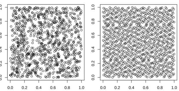
Now the concept of quasi-Monte Carlo is briefly reviewed. Quasi-Monte Carlo is often used to improve Monte Carlo estimators. In contrast to Monte Carlo, quasi-Monte Carlo integration uses so-called low-discrepancy sequences instead of (pseudo-) random numbers. Low-discrepancy numbers are constructed to fill the space more evenly. For a detailed description of the construc-tion and properties of low-discrepancy sequences the reader is referred to Niederreiter (1992) and the references given there. A nice overview is given in Glasserman (2004, Chapter 5). Pseudo-random numbers from the Mersenne Twister 19937 and quasi-random numbers from the two-dimensional Sobol sequence (Sobol 1967) are compared visually in Figure 2.3. It can be observed that, in contrast to the quasi-random numbers, the pseudo-random numbers exhibit cluster-like features.
The incentive to work with quasi-Monte Carlo is justified by its deterministic error bound of orderO(N−1logdN), which follows from the well-known Koksma-Hlawka inequality (see
Nieder-reiter (1992)). This bound is merely of theoretical benefit because the computation of the in-volved constants (including the Hardy-Krause variation of the integrand) is infeasible or at least very difficult. However, it suggests that quasi-Monte Carlo should massively outperform Monte Carlo in low-dimensional integration problems. The advantage of quasi-Monte Carlo diminishes with increasing dimension. Nevertheless, it is well-known in the financial engineering literature, that quasi-Monte Carlo may be effectively applied to high-dimensional problems (Paskov and Traub 1995; Ninomiya and Tezuka 1996; Traub and Werschulz 1998). This stems from the fact that many integration tasks in finance have rather low effective dimension compared with the nominal dimension. In Chapter 4, this is discussed in more detail.
A drawback of quasi-Monte Carlo is the lack of randomness, which impedes the computation of the mean square error for assessing the accuracy of the estimator. This issue can be resolved
0.0 0.2 0.4 0.6 0.8 1.0 0.0 0.2 0.4 0.6 0.8 1.0 0.0 0.2 0.4 0.6 0.8 1.0 0.0 0.2 0.4 0.6 0.8 1.0
Figure 2.3: Comparison of pseudo-random numbers (left plot) with quasi-random numbers (right plot). 1023 two-dimensional variates from the Mersenne Twister 19937 and from the Sobol sequence are shown.
by randomizing the deterministic low-discrepancy sequence to achieve independent realizations of the quasi-Monte Carlo estimator. Different approaches for randomizing low-discrepancy se-quences are available including Owen’s scrambling (Owen 1995), random digit scrambling (Ma-toušek 1998), or random shifts (see Ökten and Eastman (2004) for a survey). Priority is often given to the random shift technique because of its straightforward implementation. It is based on the idea to shift the entire sequence by a random vectorv modulo one. vis drawn from the uniform distribution on[0,1)d. That is, a randomized sequence is obtained by substituting the
Chapter 3
Nonparametric Importance Sampling
3.1
Introduction
In Section 2.3, the importance sampling method was described along with a discussion on the use of parametric proposals. An alternative to the classical parametric importance sampling approaches is nonparametric importance sampling. It is based on the idea to approximate the optimal proposal (or another suitable proposal) nonparametrically. The advantage of nonpara-metric methods is that, at least in low dimensions, one can expect to achieve a better approxima-tion of the optimal proposal compared with parametric techniques. In addiapproxima-tion, nonparametric importance sampling can be applied in an automatic fashion because it does not require the prior investigation of the structure of the integrand to set up a suitable parametric family of proposals.
Nonparametric approximations based on kernel estimators for the construction of proposals have been used before (West 1992, 1993; Givens and Raftery 1996; Kim, Roh, and Lee 2000). Under restrictive conditions it has been shown that nonparametric (unnormalized) importance sampling can not only reduce the variance of the estimator but may also improve its rate of convergence of the mean square error toO(N−(d+8)/(d+4))(Zhang 1996). Except for special cases,
parametric importance sampling strategies achieve the standard Monte Carlo rate of O(N−1),
because the optimal proposal is typically not included in the employed distribution family. There is still a lack of theoretical results for nonparametric importance sampling, particularly for the self-normalized importance sampler. Furthermore, computationally aspects, that critically effect the performance of nonparametric importance sampling, have only been insufficiently treated in the literature (Zlochin and Baram 2002).
The competitiveness of nonparametric importance sampling compared with parametric im-portance sampling heavily relies on the computational efficiency of the employed nonparametric estimator. In fact, until now nonparametric importance sampling is only of theoretical interest because of the computational shortcomings of the kernel estimator. In this chapter, we propose nonparametric importance sampling algorithms which are based on a multivariate frequency polygon estimator. This nonparametric estimator is shown to be computationally superior to kernel estimators. In addition, it allows the combination of nonparametric importance sampling
with other variance reduction techniques (such as stratified sampling) which is another advan-tage over kernel estimators. We investigate nonparametric importance sampling not only for unnormalized importance sampling but also for self-normalized importance sampling, which has not been done before. Under loose conditions on the integrand, the mean square error conver-gence properties of the proposed algorithms are explored (sections 3.2 and 3.3). The theoretical findings result in distinct suggestions for efficient application of nonparametric importance sam-pling. The large potential of nonparametric importance sampling to reduce Monte Carlo variance is verified empirically by means of different integration problems (sections 3.5 and 3.6). Over-all, we provide strong evidence that our nonparametric importance sampling algorithms solve well-known problems of existing nonparametric importance sampling techniques. This suggests that nonparametric importance sampling is a promising alternative to parametric importance sampling in practical applications.
3.2
A New Nonparametric Importance Sampling Algorithm
A nonparametric importance sampling algorithm based on a kernel density estimator, that ap-proximates the analytically unavailable optimal proposal qϕIS, is considered in Zhang (1996).Theoretical evidence of the usefulness of this approach has been established. In particular, it was proved that nonparametric importance sampling may yield mean square error convergence of orderO(N−(d+8)/(d+4))essentially under the very restrictive assumption thatϕphas compact
support on which ϕ is strictly positive. The theoretical results derived in this chapter require
much weaker assumptions. From a practical point of view a kernel density estimator is compu-tationally too demanding. For the purpose of nonparametric importance sampling it does not suffice that the employed nonparametric estimator provides a fast and accurate approximation of the distribution of interest. It is also required to allow efficient sampling as well as fast evaluation at arbitrary points. As a computationally more efficient alternative to the kernel estimator, it is suggested that one uses a histogram estimator (Zhang 1996). The drawback of a histogram is its slow convergence rate ofO(N−2/(2+d))compared with kernel estimators, which typically achieve O(N−4/(4+d)). Here we propose the usage of a multivariate frequency polygon which is known
as linear blend frequency polygon (LBFP) (Terrell 1983). It is constructed by interpolation of histogram bin midpoints. Though computationally only slightly more expensive than ordinary histograms, it achieves the same convergence rate as standard kernel estimators. Consider a mul-tivariate histogram estimator with bin heightfˆH
k1,...,kdfor binBk1,...,kd =
Qd
i=1[tki−h/2, tki+h/2) wherehis the bin width and(tk1, . . . , tkd)the bin mid-point. Forx∈
Qd i=1[tki, tki+h)the LBFP estimator is defined as ˆ f(x) = X j1,...,jd∈{0,1} " d Y i=1 xi−tki h ji 1−xi−tki h 1−ji# ˆ fkH1+j1,...,kd+jd. (3.1)
It can be shown thatfˆintegrates to one. A one-dimensional (linear blend) frequency polygon
3.2. A NEW NONPARAMETRIC IMPORTANCE SAMPLING ALGORITHM
h
Figure 3.1: A frequency polygon and the underlying histogram with bin widthh.
Our nonparametric importance sampling algorithm consists of two steps. In the first step the optimal proposal qϕIS given in (2.4) is estimated nonparametrically using samples drawn from a
trial distribution q0 and weighted according to the importance ratio qϕIS/q0. In the second step
an ordinary importance sampling is carried out, subject to the proposal estimated in the first step. Before we can state the algorithm we need to introduce the following quantities. LetAM
be an increasing sequence of compact sets defined by AM = {x ∈ Rd : qϕIS(x) ≥ cM}, where
cM > 0 and cM → 0 as M goes to infinity. For any function g we denote the restriction of g
on AM by gM and we abbreviate qMIS = qISϕM. Furthermore, the volume of AM is denoted by
VM. Note that, by definition,AM converges to the support ofqϕIS. The theorems in this section
consider the following algorithm (NIS).
Algorithm 1: Nonparametric Importance Sampling (NIS)
Step 1: Proposal estimation
• For j= 1, . . . , M: Sample ˜xj ∼q0. • Obtain estimate qˆMIS(x) = fˆM(x)+δM ωM+VMδM1AM(x), whereωM = 1/MPMj=1ω j M,ω j M =|ϕM(˜xj)|p(˜xj)q0(˜xj)−1, and ˆ fM(x) = 1 M hd X j1,...,jd∈{0,1} " d Y i=1 xi−tki h ji 1−xi−tki h 1−ji# × M X j=1 ωjM1Qd i=1[tki+ji−h/2,tki+ji+h/2)(˜x j) for x∈Qd i=1[tki, tki+h).
Step 2: Importance Sampling
• For i= 1, . . . , N−M: Generate sample xi from proposalqˆMIS.
• Evaluate IˆNIS
ϕM = (N−M)
−1PN−M
i=1 ϕM(xi)p(xi)ˆqMIS(xi)
−1.
The quantities AM, VM, and δM are required in the proofs of the following theorems, but
Assumption 1 Both ϕ and p have three continuous and square integrable derivatives on
supp(|ϕ|p), and|ϕ|pis bounded. Furthermore, it is assumed thatR(∇2|ϕ|p)4(|ϕ|p)−3<∞ where∇2|ϕ|p=∂2|ϕ|p/∂x2
1+. . .+∂2|ϕ|p/∂x2d.
Assumption 2 E[|ϕ|pq−01]4 is finite on supp(|ϕ|p).
Assumption 3 As total sample size N → ∞, bin width h satisfies h → 0 and M hd → ∞.
Additionally, we haveδM >0,VMδM =o(h2) and M3(VMδM)4 → ∞.
Assumption 4a cM satisfies h 8+(M hd)−2 δMc3M =o(h4+(M hc d)−1 M ) and h4+(M hd)−1 cM →0. Assumption 5a cM satisfies( R qISϕ1{qIS ϕ<cM}) 2 =o(M−1h4+ (M2hd)−1). For fixed sample size M and conditional on the samples{˜xi}M
i=1, it is not hard to show that
ˆ
IϕNISM is an unbiased estimator with variance
Var[ ˆIϕNISM] = 1 N −M Z ϕM(x)p(x) ˆ qISM(x) −IϕM 2 ˆ qMIS(x)dx. (3.2)
For the special caseϕ≥0 we haveqMIS =ϕMpIϕ−M1, and (3.2) can be rewritten as
Iϕ2M N −M Z (ˆqMIS(x)−qMIS(x))2 ˆ qISM(x) dx. (3.3)
Under the aforementioned assumptions, we now prove that the variance (3.3) attains convergence rateO(N−(d+8)/(d+4)), if bin widthh is chosen optimally.
Theorem 3.1. Suppose that the assumptions 1 through 3, 4a, 5a hold,ϕ≥0, andq =qϕIS. We obtain E[ ˆIϕNIS M −Iϕ] 2 = I 2 ϕ N−M h4H1+ 2d 3dM hdH2 ×(o(1) + 1)
and the optimal bin width
h∗= dH22d 4H13d d+41 M−d+41 , where H1= 49 2880 d X i=1 Z (∂2 iq)2 q + 1 64 X i6=j Z ∂2 iq∂j2q q , H2 = Z q q0 .
Proof. See Appendix A.1.
A direct implication of Theorem 3.1 is the following corollary.
Corollary 3.2. Under the assumptions of Theorem 3.1 and the further assumption thatM/N →
λ(0< λ <1), and h=h∗ we yield lim N→∞N d+8 d+4E h ˆ IϕNISM −Iϕ i2 =λ−d+44 (1−λ)−1×I2 ϕD and optimal proportion λ∗ = 4/(d+ 8) where
D= n (d/4)4/(d+4)+ (d/4)−d/(d+4) o h H1d(2d3−dH2)4 i1/(d+4) .
3.2. A NEW NONPARAMETRIC IMPORTANCE SAMPLING ALGORITHM
We remark that under much stronger assumptions, corresponding results for nonparametric importance sampling based on kernel estimators were obtained in Zhang (1996).
We now move to a more general case. Assume ϕ ≥ 0 (and ϕ ≤ 0) does not hold. For
this case we show that the NIS algorithm achieves the minimum importance sampling variance asymptotically. By substituting the optimal importance sampling distribution qISϕ into variance σIS2 and writing shorthand Iϕ =
R
|ϕ(x)|p(x)dx, we see the optimal variance of the importance sampling estimator to beI2ϕ−Iϕ2. Assumption 4b cM guaranties h 8+(M hd)−2 δMc5M =o(h4+(M hc3 d)−1 M ) and h4+(M hc3 d)−1 M →0. Assumption 5b cM guaranties( R qϕIS1{qIS ϕ<cM}) 2=o(M−1h2+ (M2hd)−1).
Theorem 3.3. Suppose that the assumptions 1 through 3, 4b, 5b hold,ϕdoes not have a definite sign, andq =qϕIS. Then we obtain
E[ ˆIϕNISM −Iϕ]2 = 1 N −M (I2ϕ−Iϕ2) + Iϕ2 h2H1+ 2d 3dM hdH2 ×(1 +o(1))
and the optimal bin width
h∗∗= dH22d−1 H13d d+21 M−d+21 , where H1=− R fϕ2∇8q22q + R fϕ∇ 2q 4q , H2= R q q0 −2 R fϕ q0 − R fϕ2 q0q , andfϕ = ϕp Iϕ − |ϕ|p Iϕ .
Proof. See Appendix A.4.
As a consequence of Theorem 3.3, the NIS algorithm does not lead to a mean square error rate improvement for functions ϕ, which take positive and negative values. But if the optimal
bin widthh∗∗ is used, we have
E[ ˆIϕNISM −Iϕ]2 =
I2ϕ−Iϕ2 N −M +o(N
−1).
That is, the optimal importance sampling variance is achieved asymptotically. Unlike The-orem 3.1, the optimal proportion λ cannot be computed analytically as a result of its
de-pendency on N. But theoretically, it can be computed as λ∗∗ = argminλG(N, h∗∗, λ) where
G=E[ ˆINIS
ϕM −Iϕ]
2. Clearly,λ∗∗ decreases inN. Note, that for the optimal asymptotic variance
to be achieved, it suffices that0< λ <1.
Corollary 3.2 and Theorem 3.3 suggest that importance sampling-based Monte Carlo inte-gration can be much more efficient for functionsϕ≥0(andϕ≤0) than for arbitrary functions.
This stems from the fact that for non-negative (non-positive) functions, the usage of the opti-mal proposal leads to a zero variance estimator. By approximating the optiopti-mal proposal with a consistent estimator it is therefore not surprising that the standard Monte Carlo rate can be surmounted. Consequently, it should be reasonable to decompose ϕinto positive and negative
part, ϕ = ϕ+ −ϕ−, and to apply Algorithm 1 to ϕ+ and ϕ− separately. Since then, we can
expect to achieve the superior rate O(N−(d+8)/(d+4)). Note that the partitioning of ϕ needs
not to be done analytically. It may be carried out implicitly in Step 1 of the algorithm. This approach, denoted by NIS+/-, is investigated in a simulation study in Section 3.5.
3.3
A New Nonparametric Self-Normalized Importance Sampling
Algorithm
Many problems in Bayesian inference can be written as the expectation of some function of interest,ϕ, with respect to the posterior distributionp, which is only known up to some constant.
This leads to the evaluation of integrals
Ep[ϕ] = R ϕ(x)˜p(x)dx R ˜ p(x)dx ,
where p˜= αp with unknown constant α. Self-normalized importance sampling is a standard
approach for solving such problems. It is often suggested to choose the proposal close to the posterior. But from the central limit theorem we know that one can do better by choosing it close to the optimal proposal, which is proportional to|ϕ−Iϕ|p. Next, we introduce a nonparametric
self-normalized importance sampling algorithm (NSIS).
Analogous to the definition of AM we define AeM ={x∈Rd:qϕSIS(x)≥˜cM}, where˜cM >0 and ˜cM → 0 asM goes to infinity. Its volume is denoted by VeM. The optimal proposal qϕSIS is defined in (2.6).
Algorithm 2: Nonparametric Self-Normalized Importance Sampling (NSIS)
Step 1: Proposal estimation
• For j= 1, . . . , M: Sample ˜xj ∼q0.
• Obtain estimate qˆMSIS(x) = fˆM(x)+δM
ωM+VeMδM1AeM(x), where ωM = 1/MPMj=1ωe j M, eω j M = |ϕM(˜xj)−I˘ϕM|˜p(˜x j)q 0(˜xj)−1, fˆM(x) analogous to Algorithm 1, and ˘ IϕM = PM j=1ϕM(˜xj)˜p(˜xj)q0(˜xj)−1 PM j=1p˜(˜xj)q0(˜xj)−1 .
Step 2: Self-Normalized Importance Sampling
• For i= 1, . . . , N−M: Generate sample xi from proposalqˆSIS
M . • Evaluate ˆ IϕNSISM = PN−M i=1 ϕM(xi)weM(x i) PN−M i=1 weM(x i) , whereweM(x i) = ˜p(xi)ˆqSIS M (xi)−1.
Both the self-normalized importance sampling estimator (2.3) and the NSIS algorithm pro-duce biased estimates. However, the estimates are asymptotically unbiased. Under the assump-tions 1 through 3 (withp,|ϕ|,cM,VM replaced byp˜,|ϕ−Iϕ|,˜cM,VeM) it is easy to verify that,
3.4. APPLYING NONPARAMETRIC IMPORTANCE SAMPLING
conditional on the samples {˜xi}M
i=1, the central limit theorem of Geweke (1989) holds for IˆϕNSISM (2.5). The asymptotic variance of the central limit theorem can be written as
σSIS2 = ˜Iϕ2M 1 + Z (qSISM (x)−qˆSISM (x))2 ˆ qMSIS(x) dx (3.4) with I˜ϕ M = R
|ϕM(x)−IϕM|p(x)dx being the median of ϕ. Consequently, I˜ 2
ϕM is the (asymp-totically) optimal variance that can be achieved by self-normalized importance sampling. Unless
ϕ is constant, it is impossible to build up a zero variance estimator based on self-normalized
importance sampling. This renders it unnecessary to investigate separately the mean square error convergence of NSIS for non-negative and arbitrary functions.
The structure ofσ2SISis very similar to the structure of the variance in (3.3) but the weights
e
ωMj introduce inter-sample dependencies which make the reasoning in the proofs of Theorem 3.1
and Theorem 3.3 not directly applicable. However, similarly to Theorem 3.3, we can show that NSIS attains optimal variance asymptotically for certain bin widthh and proportion0< λ <1.
Theorem 3.4. Suppose that the assumptions 1 through 3, 4a, 5a (with p, |ϕ|,cM,VM replaced by p˜, |ϕ−Iϕ|, c˜M, VeM) hold, and q=qSISϕ . Then we obtain
E[ ˆIϕNSIS M −Iϕ] 2 = I˜ 2 ϕ N−M 1 + h4H1+ 2d 3dM hdH2 ×(1 +o(1))
and the optimal bin width
˜ h∗= dH22d 4H13d d+41 M−d+41 ,
where H1 and H2 are defined as in Theorem 3.1 (with qϕIS replaced byqSISϕ ).
Proof. See Appendix A.5.
First, note that analogous to Theorem 3.3, there is no analytic solution for the optimal λ.
Second, the theorem implies that with NSIS, the mean square error rate cannot be improved. Therefore, NSIS is (at least asymptotically) less efficient than NIS+/-. There is, consequently, no reason to apply NSIS in cases where NIS+/- is applicable. However, this does not impair the usefulness of NSIS in cases when normalization is required as a result of unknown constants.
3.4
Applying Nonparametric Importance Sampling
In this section we discuss what is required for implementing NIS/NSIS. First, one needs to take care of the selection of q0, h, andλ. Second, an implementation of the LBFP estimator, which
allows the generation of samples, is required. Given these ingredients, the implementation of Algorithm 1 and 2 is straightforward.