Generalized Gaussian process models with Bayesian variable selection

Generalized Gaussian Process Models with

Bayesian Variable Selection

by

Terrance D . Savitsky

D o c t o r of Philosophy

APPROVED, THESIS COMMITTEE:

Marina Vannucci, Chair

Professor, Department of Statistics

|b^U

Peter Miiller,

Robert R. Herring Distinguished Professorship in Clinical Research,

Department of Biostatistics, University of Texas, MD Anderson Cancer Center

& C

yptirUi? kJ'. {Stf<2£f Katherine B. Ensor

Professor and Chair, Department of Statistics

ierick L. Oswald

Associate Professor, Department of Psychology

Houston, Texas

April, 2010

All rights reserved

INFORMATION TO ALL USERS

The quality of this reproduction is dependent upon the quality of the copy submitted.

In the unlikely event that the author did not send a complete manuscript

and there are missing pages, these will be noted. Also, if material had to be removed,

a note will indicate the deletion.

UMT

Dissertation Publishing

UMI 3421193

Copyright 2010 by ProQuest LLC.

All rights reserved. This edition of the work is protected against

unauthorized copying under Title 17, United States Code.

ProQuest LLC

789 East Eisenhower Parkway

P.O. Box 1346

Generalized Gaussian Process Models with Bayesian Variable Selection

by

Terrance D. Savitsky

This research proposes a unified Gaussian process modeling approach that extends

to data from the exponential dispersion family and survival data. Our specific interest is in the analysis of datasets with predictors possessing an a priori unknown form of possibly non-linear associations to the response. We incorporate Gaussian processes

in a generalized linear model framework to allow a flexible non-parametric response surface function of the predictors. We term these novel classes "generalized Gaussian process models". We consider continuous, categorical and count responses and extend

to survival outcomes. Next, we focus on the problem of selecting variables from a set of possible predictors and construct a general framework that employs mixture priors and a Metropolis-Hastings sampling scheme for the selection of the predictors with

joint posterior exploration of the model and associated parameter spaces.

We build upon this framework by first enumerating a scheme to improve efficiency

of posterior sampling. In particular, we compare the computational performance of the Metropolis-Hastings sampling scheme with a newer Metropolis-within-Gibbs al-gorithm. The new construction achieves a substantial improvement in computational efficiency while simultaneously reducing false positives. Next, leverage this efficient

scheme to investigate selection methods for addressing more complex response sur-faces, particularly under a high dimensional covariate space.

Finally, we employ spiked Dirichlet process (DP) prior constructions over set par-titions containing covariates. Our approach results in a nonparametric treatment of the distribution of the covariance parameters of the GP covariance matrix that in

turn induces a clustering of the covariates. We evaluate two prior constructions: The first employs a mixture of a point-mass and a continuous distribution as the center-ing distribution for the DP prior, therefore clustercenter-ing all covariates. The second one

employs a mixture of a spike and a DP prior with a continuous distribution as the centering distribution, which induces clustering of the selected covariates only. DP models borrow information across covariates through model-based clustering, achiev-ing sharper variable selection and prediction than what obtained usachiev-ing mixture priors

alone. We demonstrate that the former prior construction favors "sparsity", while the latter is computationally more efficient.

I would like to acknowledge my committee, Drs. Vannucci, Ensor, Muller and Os-wald, whose patient guidance and insightful questions steered my research efforts. In

particular, I thank Dr. Marina Vannucci for her mentoring and sharing her experience and creativity. I learned much about "learning how to learn" from Dr. Vannucci with intelligent use of original source materials to grow beyond coursework and where I

thought possible. Dr. Vannucci coached me to find my own creativity by consistently seeding me with suggestions to look ahead of our latest result. Additionally, Dr. Vannucci possesses a very wide knowledge of literature and generously pointed me to

seminal works to help ground my efforts. These tools around learning, creativity and thinking ahead of the immediate problem will prove critical in my next steps beyond graduation. Dr. Kathy Ensor has served as a consistent mentor for me, right from

the first days of my entry into graduate study, where she helped steel me against doubts about my ultimate success. She always makes time for students, no matter how busy, and puts people first in her role as department chair. Dr. Ensor further

supplied an important backbone in my growth as a statistician through her teaching of the mathematical statistics sequence that catalyzed an important growth in my capability. Dr. Peter Mueller expresses a model for the kind of professional I would

hope to be. He is at the same time both curious and challenging, on the one hand, and incredibly supportive and consistent on the other hand. My own intellectual curiosity grew from his comments on my work and I felt more confident for his faith

in my work. Dr. Fred Oswald supplies a broader social science perspective to the work of statistics and encourages me to think beyond models to outcomes.

Abstract ii Acknowledgments iv

List of Illustrations ix

List of Tables xiv

1 Introduction 1

2 Literature Review 7

2.1 Mixture Priors 8 2.2 MCMC for Model Selection 13

2.3 Introduction to Gaussian Process Models 16 2.4 Gaussian Process Covariance Functions 23 2.5 Introduction to Clustering with Dirichlet Processes 27

2.6 Penalized Methods 34

3 Generalized Gaussian Process Models 39

3.1 Introduction 39

3.2 Generalized Gaussian Process Model 42 3.2.1 Continuous and Categorical Responses 45

3.2.2 Count Data 49 3.3 Gaussian Process Models for Survival Data 50

3.3.1 Likelihood Function 51

3.4 Prior Model for Bayesian Variable Selection 52

3.5.1 Weak Consistency of Posterior Distribution 55 3.5.2 Markov chain Monte Carlo Algorithm 56 3.5.3 Metropolis-Hastings Equivalence with Reversible Jump . . . . 61

3.5.4 Posterior Prediction 64

3.5.5 Survival Function Estimation 65

3.6 Computational Aspects 66 3.6.1 Hyperparameter Settings 66

3.6.2 Projection Method for Large n 67

3.7 Simulation Study 68 3.7.1 Use of Variable Selection Parameters 68

3.7.2 Large p 70

3.7.3 Large n 74 3.7.4 Interaction Terms 76

3.7.5 Including Quadratic Covariance Term 77

3.8 Benchmark Data Applications 79

3.8.1 Ozone d a t a 79

3.8.2 Boston Housing data 81 3.8.3 DLBCL Failure Time Data 84

3.9 Discussion 87

4 Computational Strategies 89

4.1 Introduction 89 4.2 1-term vs. 2-term Covariance 91

4.3 Prior Model for Bayesian Variable Selection 92

4.4 Markov Chain Monte Carlo Methods 95

4.4.1 Metropolis Hastings 96 4.4.2 Metropolis within Gibbs 98 4.4.3 Adaptive Metropolis within Gibbs 103

4.5 Computational Aspects 105 4.6 Simulation Study 107

4.6.1 Hyperparameter Settings 107 4.6.2 Performance Comparison of MCMC Schemes 108

4.6.3 1 vs. 2-term Covariance 114

4.6.4 Selecting Covariance Terms vs. Selecting Covariates 116

4.6.5 Identifiability for Covariance Parameters 121

4.7 Benchmark Data Applications 124

4.8 Discussion 126

5 Clustering for Generalized Gaussian Process Models 128

5.1 Introduction 128

5.2 Spiked Dirichlet Process Prior Models for Variable Selection 131

5.2.1 Clustering All Covariates 133 5.2.2 Clustering Selected Covariates 134

5.3 Prior Model for Clustering Observations 135 5.4 Markov Chain Monte Carlo Methods 136

5.4.1 Clustering All Covariates 138

5.4.2 Clustering Selected Covariates 140

5.5 Simulation Study 142 5.5.1 Hyperparameters Setting 142

5.5.2 Clustering vs. No Clustering 143 5.5.3 Clustering All vs. Selected Covariates 144

5.5.4 Clustering Covariates and Observations 146

5.6 Benchmark Data Application 148

5.7 Discussion 152

6 Conclusion 154

A p p e n d i x 166

A 167

A.l Derivations for Multivariate Models 167

1 Density functions constructed from Mixture Prior of George &; McCulloch (1993). Each plot shows two density functions obtained

from each component of the mixture prior. The component

concentrated on 0 uses standard deviation, r = 0.1, while the diffuse

component component employs multiplication factor, c = 10 9

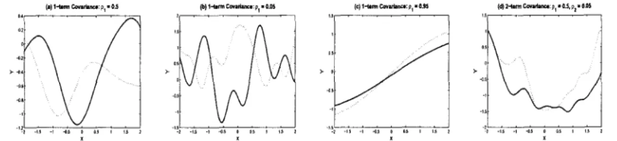
2 Response curves drawn from a GP. Each plot shows two (solid and dashed) random realizations. Plots (a) — (c) were obtained by

employing the exponential covariance (2.18) and plot (d) with a

2-term formulation. All curves employ a single dimension covariate, x 20

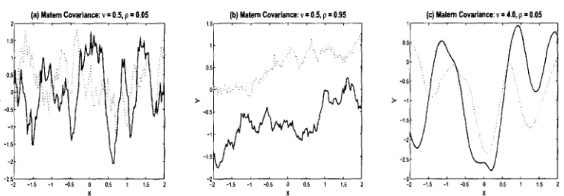
3 Response curves drawn from a G P using Matern covariance. Each plot shows two (solid and dashed) random realizations. Plots (a) — (c) were obtained by employing the Matern covariance (2.19)

with varying values for the smoothness parameter, u, and covariance

parameter, p. All curves employ a single dimension covariate, x. . . . 27 4 Conceptual Illustration of G ~ D P ( a , Go) using Sethuraman (1994).

G is composed of an infinite collection of point masses 4>k with

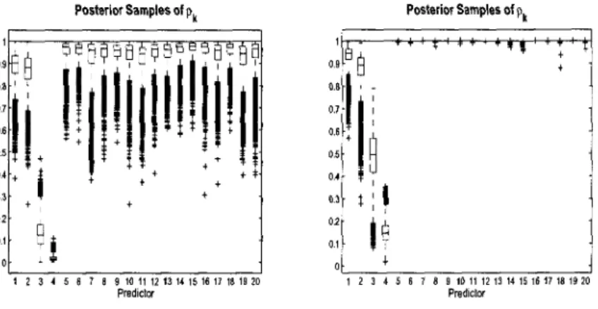
3.1 Use of Variable Selection Parameters: Simulated data

(n — 80,p = 20). Box plots of posterior samples for pk G [0,1]. Values

closer to 0 indicate stronger association to the response. Upper

(lower) plot demonstrates selection without (with) the inclusion of

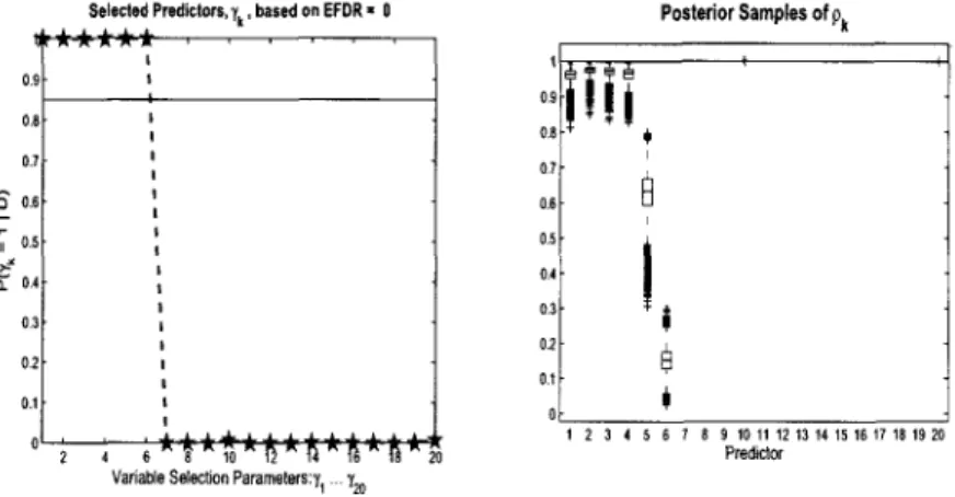
the selection parameter, 7 , in the model 70 3.2 Continuous Data Model Variable Selection: Simulated data

(n = 100,p = 1000). Posterior distributions for 7^ = 1 and box plots

of posterior samples for pk. First six covariates should be selected. . 74

3.3 Count Data Model Variable Selection: Simulated data

(n = 100,p = 1000). Posterior distributions for 7fc = 1 and box plots

of posterior samples for pk. First six covariates should be selected. . 75

3.4 Cox Model Variable Selection: Simulated data (n = 100,p = 1000). Posterior distributions for 7^ = 1, box plots of posterior samples for Pk and average survivor function curve for validation set (the dashed line) compared to Kaplan-Meier empirical estimate (the solid line).

First six covariates should be selected 75 3.5 Large Sample size (n): Simulated data (n = 300,p = 1000).

Continuous data simulation generated in same manner as Figure 3.2. Top left plot shows posterior distributions for 7^ = 1 for variable selection parameters would select correct predictors. Box plot posterior samples indicate only the actual predictors demonstrate

association to the response 76

3.6 Inclusion of Interaction Terms: Simulated data (n — 120,p = 1000). Continuous data simulation generated in same manner as Figure 3.2. Box plots of posterior samples for pk demonstrate selection of the

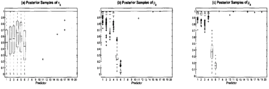
3.7 Covariance with Linear Term for Weak Signal: Simulated data (n = 100,p = 1000). Plots (a), (b), (c) display box plots of posterior samples for uk,Pk for covariance formulations including ((a), (6)) and

excluding ((c)) the quadratic covariance term. First six covariates

should be selected 79

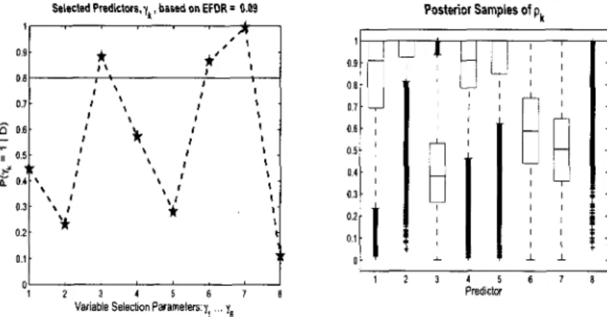
3.8 Count Data Model Variable Selection: Ozone Benchmark data. Posterior distributions for jk = 1 and box plots of posterior samples

for pk. Projection method used with m/n = 0.25 82

3.9 Continuous Data Model Variable Selection: Boston Housing

Benchmark data. Posterior distributions for jk — 1 a nd box plots of

posterior samples for pk. Projection method used with m/n = 0.25. . 84

3.10 Cox Model Variable Selection: Rosenwald et al. (2002) DLBCL data. Average survivor function curve for validation set (the dashed line)

compared to Kaplan-Meier empirical estimate (the solid line) 86

4.1 Count Data Variable Selection under MCMC schemes: Simulated data (n = 100,p = 1000). Posterior distributions for jk = 1, box plots

of posterior samples for pk from Metropolis-Hastings algorithm (top)

and Gibbs scheme (bottom) I l l 4.2 Autocorrelation for Selected Parameters, pk: Simulated data

(n = 100,p = 1000). Autocorrelation for posterior samples of pk,

comparing a mixture of uniforms proposal to the usual [7(0,1). . . . 115

4.3 2-Term covariance, 1 set of selection parameters. Simulated data. Posterior p(-yk = 1|-D) and box plots of posterior samples for p\tk and

P2,k 116

4.4 2-Term covariance with 2 sets of selection parameters: Simulated data. Posterior p^i^ = 1|D) & p{^2,k — 1|-D) and box plots of

4.5 2-Term covariance, 1 set of selection parameters. Simulated data. Posterior p(jk = 1|D) and box plots of posterior samples for p\tk and

P2,k H 9 4.6 2-Term covariance, 2 sets of selection parameters. Simulated data.

Posterior p(ji,k = 1\D) & p(l2,k = 1|-D) and box plots of posterior

samples for p ^ and p2,k 120

4.7 2-Term covariance, 1 set of selection parameters. Simulated data.

Posterior p{"fk = l|-0) and box plots of posterior samples for pi}k and

p2,k 122

4.8 2-Term covariance, 2 sets of selection parameters. Simulated data.

Posterior piji^ = 1|-D) & p(j2,k = 1|£>) and box plots of posterior

samples for pi^ and p2tk 123

4.9 2-Term covariance, 2 sets of selection parameters. Simulated data.

Posterior p(j\tk = 1|-D) & p(j2,k = 1|-D) and box plots of posterior

samples for p\k and p2,k 124 4.10 Boston housing benchmark data. Marginal posterior probabilities of

7^ = 1 and box plots of posterior samples for pi)fc,p2,fc 125

5.1 Effect of covariate clustering employing prior model (5.5): Univariate regression model (n = 130, p = 1000). Box plots of posterior samples

for the p;t's; (a) shows results without covariate clustering; (b) shows

results with covariate clustering 144

5.2 Effect of covariate clustering: Survival model (n = 150, p = 1000).. Box plots of posterior samples for the p^'s and marginal posterior probabilities for the 7fc's; (a) and (c) show results with clustering of

all covariates; (b) and (d) show results with clustering of only selected

3 Effect of Clustering on both Covariates and Observations: Univariate Regression simulation (n = 130, p = 1000). Posterior samples of p.

Plots (a) — (c) display box plots for pk under covariance (3.5); (a) Without clustering models; (b) With clustering on all covariates -selected and trivial (c) With clustering on only -selected covariates.

Includes clustering model on error term precisions 147 4 Covariate Clustering: Boston Housing Benchmark data. Posterior

samples of p. Plots (a), (b) present box plots of pk; (a) Without

clustering models; (b) With clustering on all covariates 149 5 Benchmark Data Application. Box plots for posterior samples of the

Pfc's and predicted survivor functions compared to Kaplan-Meier estimates; (a) and (c) show results without covariate clustering; (b)

3.1 Simulations:

y = a\X\ + 0,2X2 + 03X3 + (I4X4 + fl5 sin(a6^5) + 0,7 sin(agX6) + e . . . . 72

3.2 Ozone Data: Variables Description 80

3.3 Ozone Data: Results 81 3.4 Boston Housing Data: Variables description 83

3.5 DLBCL Failure Time Data: Top 10 Genes Associated to Survival Time 85

4.1 Continuous data simulation from model (4.15) 110

4.2 Count data simulation from model (4.16) I l l 4.3 Count data simulation from model (4.16) under correlated variables. . 112

Chapter 1

Introduction

This research supplies a newer Bayesian construction to better accomplish response

surface generation and variable selection under a covariate space composed of a

het-erogenous mix of lower and higher order associations to an observed or latent response

than is possible using the popular linear variable selection methods, both Bayesian and

classical. The simultaneous selection of covariates and response surface construction

in a supervised setting are among the most common problems that appear in broad

areas of research from biomedical applications, on the one hand, to social science and

business experiments, on the other hand. Acquisition of subjects for biomedical

ex-periments, including pharmaceutical clinical trials, is difficult and relatively expensive

which tends to keep sample sizes, n, low. The associated measurement of covariates,

such as gene expression intensities, however, are relatively inexpensive and result in

sometimes thousands of covariates associated to each subject, thus setting up the

well-known statistical challenge to conduct inference for data sets characterized by

n <C p; (see Sha et al. (2006) for examples of time-to-event gene expression data sets where n <C p). Brain imaging experiments which record neural impulse expression

intensities supply another set of high dimension covariate space examples. The

di-mension of covariate spaces under these type of experiments is likely to continue to

grow as studies incorporate longitudinal public health data and other environmental

variables to complement gene expression data in an attempt to capture more the

As biomedical experiments increase the scope of genetic data employed, as well as

including environmental data, there is a greater likelihood that some or many

covari-ates will express non-linear associations to a dependent response. When variables are

all of the same type, it is sometimes possible to apply a linearizing transformation to

accommodate application of easier-to-estimate linear statistical models; for example,

expressions of gene intensities are normalized with division by typical/normal

expres-sion levels and linearized with a logarithm transformation. Some may argue that

important distinctions in the d a t a may be lost by such strong transformations, which

may impact subsequent selection and prediction results. When the covariates are of

different types, a characteristic referred to as "heterogenous", it may not be at all clear

how to execute a linearizing transformation. While not typically characterized by high

dimension covariate spaces, social science data may combine lab-based experimental

measurements with observational data, producing a covariate space characterized by

a large degree of heterogeneity; see Long (1997) for examples. Such data as these call

for methods that directly account for heterogeneity of the covariate space.

Chapter 2 presents a review of the development of statistical methods for variable

selection. We briefly mention, here, the development of linear Bayesian variable

selec-tion models designed to address the n <C p problem. This construcselec-tion accomplishes

simultaneous response surface generation and variable selection under generalized

lin-ear models in a manner that accommodates low n and efficiently handles high p. In

particular, we see that the constructions of Smith & Kohn (1996) and Brown et al.

(1998, 2002) employ fully conjugate (univariate and multivariate) regression

mod-els in both the variance and mean, enabling marginalization over the error variance

and slope parameters under a linear model construction. Such models employ a set

slope coefficients that is conditional on whether a given covariate is included or

ex-cluded from the model space). A closed form expression is achieved for the joint

posterior over the space of models, up to a normalization constant. This fortuitous

outcome allows for computationally-efficient posterior sampling (through exploration

of the space of models) and readily accommodates low sample sizes. A particular

fea-ture of these linear Bayesian variable selection constructions is that they account for

model sparsity by automatically incorporating a multiplicity correction penalty

with-out compromising ease to conduct posterior inference; see Scott &, Berger (2008). The

linear Bayesian variable selection construction is now a standard method employed

to conduct variable selection and prediction and is one important driver for such

transformations of the covariate space as the logarithm transform for gene intensity

expression data to allow the data to fit the model.

With the development of models that employ a Gaussian process (GP) prior

con-struction in a Bayesian implementation, in lieu of the noted linear concon-struction, we

remove the requirement to conduct a linearizing transformation of the covariate space

to directly accommodate variable selection and prediction under heterogenous

covari-ate spaces. The Gaussian process construction allows each covaricovari-ate to express a

low-to-high order association to the response in joint estimation with all other

co-variates. The result is a method that produces response surfaces spanning the space

of mathematically smooth functions based on the chosen parameterization for the

covariance matrix of the Gaussian process prior construction. This covariance matrix

may be arbitrarily complex. We may even employ a covariance matrix formulation

(Matern) that uses an explicit smoothness parameter to allow response surfaces of

fractal expression. A particular feature of the Gaussian process variable selection

the functional form that relates the covariates to the response. The construction for

the probability model allows the data to select the form in posterior updating.

As with the linear construction, the Gaussian process prior is employed for the

exponential dispersion family under the generalized linear model framework, a

formu-lation labeled in this research as "generalized Gaussian process models". As with the

linear construction, a set of {0,1} parameters are introduced to index the model space

to accomplish variable selection. While the generalized Gaussian process models

en-joy the same theoretical properties as the linear case, including supplying multiplicity

correction, the greater complexity of this construction produces a non-conjugate

for-mulation disabling the marginalization over the parameter space associated to the

model space. This research adapts, modifies and extends MCMC sampling methods

(of Madigan k York (1995), Gottardo & Raftery (2008), Neal (2000)) to the

Gaus-sian process construction to accomplish a set of relatively efficient posterior sampling

schemes.

The implementation of posterior sampling schemes for generalized Gaussian

pro-cess models in this work also includes data structure innovations that produce

suf-ficient computational efficiency to accommodate high dimension covariate spaces.

These innovations focus on reducing multivariate computations to a set of easily

ac-complished inner products, which are optimized with application of linear algebra

libraries.

Of course, rarely is one able to get "something for nothing", meaning although

the generalized Gaussian process models produce a more general construction for

accommodating non-linearities than does the linear construction and equally

accom-modates high dimensional covariate spaces, the greater complexity tends to require

thesis adapts and develops efficient methods to reduce the computational intensity

to conduct matrix decompositions required to compute the inverse of the Gaussian

process covariance matrix. These innovations reduce computation time (of 0(n3))

to invert the G P covariance matrix so that the construction in this work is able to

address higher sample sizes than the n = 1000 suggested by Neal (1999). Yet, the

generalized Gaussian process construction is not well-suited to n larger than a few

thousand. There still remain a large class of data applications with large p in a

heterogenous covariate space that are addressed in the sequel.

Context for the research captured in this thesis is supplied with a literature review

in Chapter 2. The chapter sketches the development of Bayesian variable selection for

linear models, including the development of posterior sampling algorithms. Gaussian

process models and associated forms for covariance matrices are introduced. Classical

methods to accomplish variable selection, including the Lasso of Tishirani (1996) and

elastic net of Zou & Hastie (2005), are reviewed. Lastly, this chapter concludes with an

overview of Bayesian non-parametric formulations for clustering models that will be

coupled with the generalized Gaussian process formulation. This thesis next develops

a methodological core that includes enumeration of the generalized Gaussian process

models in Chapter 3 equipped with Bayesian variable selection to simultaneously

ac-complish variable selection and response surface generation. A full complement of

univariate and multivariate generalized Gaussian process models are developed for

continuous, categorical and count data. The model framework is also extended to

the multiplicative hazard model of Cox (1972) for time-to-event data. Lastly, this

chapter supplies a substantial modification to the Metropolis-Hastings posterior

sam-pling method used for linear data to accommodate the joint samsam-pling of model and

is expanded in Chapter 4, first, by adapting and applying a new

Metropolis-within-Gibbs scheme to more efficiently conduct posterior inference. This scheme is then

leveraged under a more complex covariance structure and selection construction,

de-veloped in this chapter to address a broader class of possible response surfaces; in

particular, to accommodate high non-linearity across multiple covariate dimensions.

The generalized Gaussian process framework is next equipped in Chapter 5 with prior

constructions that permit clustering of covariates to strength variable selection and

also to generalize the distribution construction of the error term for continuous data

C h a p t e r 2

L i t e r a t u r e Review

This research effort addresses a rather classic problem; selecting covariates related

to an (observed or latent) response from among a large set of candidates. We focus

our efforts on Bayesian methods to simultaneously select covariates and construct

a response surface under the usual set of data types, including continuous, count,

categorical and event time observed data. The formulations for the set of probability

models and associated posterior sampling algorithms to accomplish selection are

col-lected in the term, Bayesian variable selection (BVS); see Brown et al. (1998). The

following section will supply context and introduce the core BVS concepts we will

later employ in our work. We begin this section with an overview of the mixture

prior construction that enables posterior sampling within the space of (2P) possible

covariate models that may be formed from p candidate covariates. We will learn

in the sequel how the recent evolution of the mixture prior formulation provides a

theoretically robust and practical formulation for addressing multiplicity correction.

We next briefly examine how this prior construction is employed in linear continuous

data regression to accomplish Bayesian variable selection. The evolution of

associ-ated Markov chain Monte Carlo (MCMC) methods to sample the resulting posterior

mixture under the linear model formulation are reviewed. We next introduce the

Gaussian process modeling focus our research as a capstone to tie together and

il-lustrate our use of BVS methods. We first motivate the use of Gaussian process

formulation and then introduce a more general covariance formulation that allows

us to build response surfaces of arbitrary complexity within the space of

mathemat-ically smooth functions. We employ this covariance formulation to illustrate a more

generalized G P univariate regression model. We next conduct a review of the family

of weakly stationary covariance matrices we may utilize in our G P variable selection

models. Also included is an introduction to clustering using a Dirichlet process (DP)

formulation. We construct DP probability models and enumerate the posterior

sam-pling procedures under conjugate and non-conjugate models. Inclusion of this topic

stems from our later development of GP probablity models that address clustering on

both covariates and observations to enhance the performance of our model selection

and robustify the distribution over error or random effects terms, respectively. This

section concludes with an overview of the lasso and elastic net penalized likelihood

methods to perform variable selection as an alternative to BVS. Classical methods

are introduced, as well as a Bayesian construction for the elastic net. Comparisons

of posterior sampling methods between the BVS and Bayesian elastic net models are

discussed.

2.1 Mixture Priors

Introduce the univariate linear regression formulation with the likelihood, y|/3, a2 ~

Af(X.(3, cr2In), for n x 1 response, y and nxp design matrix, X with (3 = (/3i,..., /3P)

associated to each of the p covariates. In is an n x n identity matrix. In the original

formulation of George &; McCulloch (1993), a mixture prior formulation is placed on

Mixture Prior for 0: i = .1, c = 10

Figure 2.1 : Density functions constructed from Mixture Prior of George k, McCulloch (1993). Each plot shows two density functions obtained from each component of the mixture prior. The component concentrated on 0 uses standard deviation, r = 0.1, while the diffuse component component employs multiplication factor, c = 10.

where k = 1 , . . . ,p, p the number of candidate covariates. Introduce % 6 {0,1} to

index the model space, T = { 7 1 , . . . , 7 2 P } , where |T| = 2P. The variance parameter,

r | is chosen sufficiently small such that the mixture component associated to jk = 0

is concentrated around 0, meaning that associated covariate, xk is effectively excluded

from the model. A further prior bernoulli prior is imposed for jk\a ~ Bern(a), where

a is the a priori probability for inclusion of xk in the model.

In particular, the use of Lebesgue measures - instead of simply choosing a Dirac

measure that would set fik = 0 for 7*, = 0 - was chosen to retain a fixed dimension,

p, for visited model spaces for ease of posterior sampling. Figure (2.1) illustrates the mixture prior for r = 0.1 and multiplication factor, c = 10. We may place further

priors on r and c, though George & McCulloch (1993, 1997) suggest using the desired

width, 6, formed from the intersection of the two components to choose these values.

from which we may conduct posterior sampling. Carlin & Chibb (1995), Smith &

Kohn (1996) and George & McCulloch (1997), among others, evolve this mixture

prior to allow for the explicit exclusion of covariate, Xk, using the construction,

fa\lk, i>fc ~ (1 - lk)50 + ik AA(0, vk), (2.2)

where So is a Dirac measure which places point mass at 0. While this model more

readily allows for covariate exclusion and reduces the number of hyperparameters

to be tuned or estimated a posteriori, the dimension of the model and associated

parameter spaces now change based on which covariates are excluded from a given

model. We will discuss implications of the changing dimension for the model space

in the next section where we review MCMC methods.

Introduce (3y where fatl = fa if jk — 1 or faa — 0 if jk = 0 to allow the vector of

regression coefficients to vary in dimension for specific model, 7 . Then re-state the

probability model for linear regression from Smith & Kohn (1996) and Liang et al.

(2008) employing conjugate prior formulations,

n x l nxp^pyXl y = X7 / 37 + e (2.3) e ~ Af(0,a2In) (2.4) p{a2) oc \ (2.5) / 3 >2 ~ ^ ( ( ^ ( X p g - 1 ) (2.6) y\a ~ 0^(1-a)*-1* (2.7)

where a2 is the error term variance parameter and p7 < p captures the number of

covariates in model 7 and I„ is the n x n identity matrix. The prior formulation

for /37|<T2 sets Vk = go-2 ( X ^ X7) in the mixture prior formulation of (2.2), a

incorporates the least squares estimate for the variance of (3. The parameter, g, scales

the prior variance for (3 and is typically set to produce a diffuse distribution. We may

also place a further prior on g to instantiate a fully Bayesian construction, the

impli-cations of which we will discuss further, below. Collect parameters in 0 7 = (/37, a2).

Scott & Berger (2008) show multiplicity correction for the implied multiple

hy-pothesis test is provided in the resulting marginal prior construction on 7 achieved by

placing a 13(1,1) weak uniform prior on a to establish a fully Bayesian construction,

7r(7) = f17r(7\a)7T(a)da = - J - ( P ) (2.8)

Jo p+l \p-fj

This marginal prior induces a non-linear (decreasing) penalty for adding an extra

covariate for a given-sized model space; for example, when moving from the null

model to a model with one covariate, the log-prior favors the null model by a factor

of 30 for p = 30. The penalty increases with the dimension of the model space, p. In

practice, fixing a < 0.5, which is typical under prior expectation for model sparsity,

supplies multiplicity correction as also noted by Scott & Berger (2008); also see Brown

et al. (1998) among many others. We conclude that the mixture prior formulation

automatically adjusts for multiplicity without the requirement to explicitly introduce

a complexity penalty term.

Compute the marginal posterior for model 7 ,

P(Y|7) = f p<y\ejp{0Md6^ (2.9)

from which we compose the Bayes factor, the ratio of posterior probabilities given

models 7 and 70, respectively, to compare model, 7 with the null model, 70 =

( 0 , . . . , 0 ) ,

where R^ is the coefficient of determination for regression model, 7 . (Note that we

may accommodate p > n by replacing p7 with the rank of the projection space,

X y X ^ ) . Smith & Kohn (1996) observe from (2.10) that fixing a value for g where a

large value is chosen for noninformativeness favors the null model as g —> 00 when

n and p7 are also fixed; a phenomenon termed Bartlett's paradox. Another

asymp-totically inconsistent result when using fixed g, termed the Information Paradox is

also observed from (2.10). As we accumulate overwhelming support for model, 7 ,

we expect i?7 —>• 1, meaning the associated F— statistic goes to 00; but we see that

(n — p-y — 1)

(2.10) tends to a constant, (1 + g) 2 for a fixed g. Liang et al. (2008), however,

show these inconsistencies are resolved when either an empirical Bayes (maximum

likelihood) estimate or a fully Bayes model is utilized by placing a continuous prior

on g. Again, in practice, Smith & Kohn (1996) show that choosing relatively large

fixed values for g E [10,1000] produce good selection results.

Lastly, we note a result from Brown et al. (2002) that suggests to utilize an

independent diagonal construction for the prior variance on / 37, [pcr2]IPT, in lieu

of the usual [gcr2] ( X ^ X7) when X7 is ill-conditioned due to a highly correlated

covariate space. Suppose our design matrix is of rank r < p. Employ the singular

value decomposition (SVD) to isolate unstable directions,

X = U D Vr, (2.11)

for n x p design matrix, X, where n x r matrix U and p x r matrix V are column

orthonormal and D is diagonal matrix with entries the square root of the non-zero

reformu-lated regression model,

m3- = y/TjOj + ej (2.12)

83 ~ Af ( o , - ^ r2) , (2.13)

where A., is the jt h eigenvalue of X ^ X7 for j = 1 , . . . , r. Finally, derive E(6j\rrij) =

[g/(l + g)] OJ,LS, where O^LS is the least-squares solution. Alternatively, if we employ

the diagonal prior construction, then E(9j\irij) = [A_,-/(Aj + g)\ OJ,LS- From this

pos-terior expectation under the g—prior we see that the shrinkage factor retains much

more information on ill-conditioned directions whereas the diagonal prior

construc-tion readily shrinks these direcconstruc-tions (due to small Aj) to 0. We conclude that the

use of g—prior should be replaced with the diagonal prior construction under an

ill-conditioned design matrix.

2.2 M C M C for Model Selection

The original mixture prior formulation of George & McCulloch (1993) expressed in

(2.1), is non-conjugate, which explains the choice of a Lebesgue measure for both

components; the desire to maintain constant dimension between proposed moves in an

MCMC for /3, which must be directly sampled a posteriori. An important method for

posterior sampling under moves across changing dimensions for the parameter space

is the reversible jump of Green (1995). To gain a brief insight into the construction

of this method, describe the probability of move between x = (1, 9^) G C\ to x =

(2,0(2)) G C2, where we assume space, C2 is of higher dimension than C\. We first

randomly generate u^ of length p\ = \C2\ — \C\\ (the difference in dimension between

the larger and smaller spaces), independently of 8^ and then set 8^ equal to some

move (from a set of possibilities) from x to x and analogously for j(\,6^). Then we

may express the probability of move as,

m i n a

<r(2,*»ta,y(2,*»)

d{oM)

d(0W,uW)

where 7r(2,0^\y) is the posterior probability for 6^ G €2- The last term is the usual

Jacobian associated to transforming from one space to another. In practice, this

construction may require definition and associated computation for multiple move

types, (e.g. "split", "merge", "birth", "death"), to achieve acceptable chain mixing,

so other less complicated constructions are often substituted.

Though the mixture construction of Lebesgue measures from George &; McCulloch

(1993) avoided a parameter space dimension change, it proved difficult to set the

variance parameter, r , in (2.1) sufficiently large enough to produce a fast converging

chain, while being set adequately small to effectively exclude nuisance covariates. The

result was a slow-converging Gibbs sampler for (3.

Carlin & Chibb (1995), Smith & Kohn (1996) and George k McCulloch (1997)

subsequently defined conjugate probability models using the mixture prior with a

Dirac measure component shown in (2.2) and the prior over j3 in (2.7). The fully

conjugate model through both mean and variance allow marginalization over both

/37 and a2 achieve the following posterior construction for the {0,1} model space

indicators, 7 ,

7 r (7| y ) <x TT(7) I L ( y | / 37, a > ( / 3 > V ( a2) d / V ^2 (2-14)

c< 5 (7) = (l + c ) " ^/ 25 (7) - " /2, (2.15)

where S(-f) = y ' y — [c/(l + c ) ] y ' X7( X !yX7) "1X7' y - Now we are left to only

sam-ple this posterior construction on 7, a vector of bernoulli random variables where

and Brown et al. (1998) developed alternative transformations of ( y , X7) to

sup-port fast computation of (2.15) for posterior updating. Brown et al. (1998)

em-ploy a component-by-component, Metropolis-within-Gibbs algorithm, but switch to

a joint updating for 7 with a Metropolis-Hastings scheme in Brown et al. (2002). The

Metropolis-Hastings scheme is based on the model comparison, or MC3, algorithm of

Madigan & York (1995) and proposes a new model through a random exploration of

the model space. Randomly choose between two move types that change one or two

components in 7 ; the moves are defined as,

1. A d d / D e l e t e : Randomly choose 7 ^ 7 = { 7 1 , . . . ,jp} and propose j 'k = 1 if

7fc = 0 or vice versa.

2. S w a p : Perform both an Add and Delete move for randomly chosen positions,

ke{l,...,p}.

This construction produces a symmetric proposal density, 5 ( 7 , 7 ) = 9(7 , 7 ) , so that

the probability of move reduces to,

It is well to note that though only one or two components are changed on each

iteration, the entire model, 7 , is proposed. A random exploration of the model space

proves more efficient than a component sampling Metropolis-within-Gibbs approach

in this special case. Repeated visits to the same model during posterior sampling are

duplicate since we have marginalized over the parameter space (which is absolutely

continuous with respect to the Lebesgue measure). The availability of (2.15) to

compute the joint posterior for each model (up to a normalization constant) means

of these two observations is that we only require the chain to visit a model of high

posterior density once, so that we don't need convergence in our stochastic search

over the posterior space and use the MC3 algorithm to produce a well-mixing chain,

resulting in chains with fewer iterations.

2.3 Introduction to Gaussian Process Models

We develop a model formulation based on Gaussian processes to supply a more

gen-eral non-parametric framework for simultaneously generating the response surface

(for an observed or latent response) and accomplishing variable selection. Our work

leverages BVS methodology, but broadens the class of response surfaces that may be

constructed, formulates new probability models that employ a mixture prior

construc-tion for robust variable selecconstruc-tion, and provides new computaconstruc-tionally-efficient Markov

Chain Monte Carlo (MCMC) algorithms to jointly sample model and associated

pa-rameter spaces. In particular, our construction imposes a Gaussian process prior

function of covariates in, for example, the univariate regression model, y = z(X) + e,

where:

z ( X ) | C ~ J V ( 0 , C ) . (2.16)

Then, z(X) is an n x 1 realization of a Gaussian process with covariance matrix,

C. We may produce a response surface of arbitrary complexity within the space of

continuous surfaces of any order of differentiability based on how we parameterize C.

It will be further shown how we may even use this more general prior construction to

produce the linear model. Most satisfying, we are able to embed our new framework

within the generalized linear model framework of McCullagh & Nelder (1989) to

produce a semi-parametric formulation for the regression problem with an either

process models. One variation of our model employs a mixture of Dirichlet processes

as enumerated in Antoniak (1974) to allow clustering of observations that provides

a nonparametric formulation for the error term in a regression model or the random

effects in a generalized Gaussian process mixed effects model. In such case, we provide

a fully nonparametric formulation for continuous data regression.

The use of Gaussian process regression models are recently common in machine

learning approaches and spatial applications as a means to generalize the function

relationship between predictors and a response; see Rasmusen & Williams (2006) and

Linkletter et al. (2006). The statistical applications emerged due, in large part, from

the work of Neal (1996), who showed that Bayesian regression models based on neural

networks converge to Gaussian processes in the limit of an infinite network. Early

ap-plications in statistics may be found in O'Hagan (1978). The emergence of Gaussian

process regression and classification models for spatial data coincided with the

imple-mentation of the exponential covariance function as described by Sacks et al. (2000)

and Neal (1999). This covariance function is an anistropic construction based on the

squared Euclidean distance among the set of covariates associated to observations, so

that two observations with similar covariate locations would be expected to produce

similar response values; a continuous construction very appropriate for spatial data.

Recently, however, Banerjee et al. (2008) apply the more general Matern covariance

formulation that implements a separate smoothness parameter allowing for rougher

(though continuous) processes.

the approach of Neal (1999) and begin with the linear regression model, v

Vi =

+ Yl

i,kPk + Si

ex ~ Af{0,a2£),a~Af(0}a2a),

from which we extract the dot product covariance function,

Cov(yi,yj) = dj = E {a + J2

hkPk + £i) f a + J2

i,kh + £•» j

= al + Y, xi,kX3Mal +

tijVe-fc=l

We achieve covariance n x n covariance matrix, C = a\J„ + X H X + a2In, with Jra a

matrix of l's and In the identity matrix and H = diag ( o f , . . . , a2). Marginalize over

{/3, a, e} by simply summing over Gaussian priors to define a Gaussian likelihood on

y|cr^,,H,c7| with covariance C . Place a further set of priors on {<7^,,H, crjj:}. We've

now defined a Gaussian process probability construction from which we may sample

posterior distributions through the priors on the these parameters and the likelihood

on y; of course, we would not employ this construction for the linear model due to

the added computational burden to generate C, though we have performed the most

basic and intuitive construction for the GP probability model.

We are able, however, to generalize the construction for C in the GP formulation

to allow for more interesting, mathematically rougher response surfaces within the

space of continuous functions; see Rasmusen & Williams (2006). Construct a more

general probability model from Savitsky et al. (2009a) with,

n x l

y = z(X) + e

z(X) = ( z ( x

) , . . . , z ( x

) ) ' ~ ^

( 0 , C )

e - AT

(o, [ \ ] ) ,

where z is an n x 1 realization of a Gaussian process with covariance, C. We may

marginalize over z and e, as before to provide the likelihood,

y f c ! r ~ A / ; ( 0 , [ \ + c ] ) (2.17)

We employ an exponential covariance term, formally introduced in Chapter 3,

which is related to the formulation of Linkletter et al. (2006),

C = Cov(z(X)) = ~3n + f e x p ( - G ) , (2.18)

where G = {gij} with elements <?»,, = (XJ—Xj)'P(x,— Xj) and P = diag (— l o g ( p i , . . . , pp)),

with pk G [0,1] associated to Xk, k = 1 , . . . ,p; AQ and Xz are precision parameters

associated to the regression intercept and weight on the non-linear exponential term,

respectively. To better understand this construction, extract a cell from C,

1 1 P ( ^2

^ij - T~ + T~ 11 Pk

Aa *z k=i

We readily note that when pt~ = 1, covariate xk doesn't influence y (through C),

a designed property we will later employ to accomplish variable selection. The

for-mulation of Savitsky et al. (2009a) is a transformation of the covariance function of

Sacks et al. (2000), Q j = I H U I exp(—6k\xik — Xjk\R), where we define pk = exp(—6k)

for 6k £ [0, oo) and set R — 2; the latter choice for smoothness we will review in

more detail, shortly. The exponential covariance function derives from the family of

translation invariant or stationary covariance functions and supplies a parsimonious

formulation to capture both lower and higher order non-linear surfaces. In particular,

this construction also incorporates the linear response modeled by the special case

dot product covariance. Figure 2.2 provides a graphical illustration of the types of

surfaces captured by Gaussian processes. The two lines in each chart are random

(•) 1-torm Covarknc*: p, • 0.5 (b) 1-torm Covarianct: p( • 0.0S (c) 1-terni Covariaiwt: p,» 0.95 (d) 2-lerm Covartance: p, • 0.5, p( • O.M

Figure 2.2 : Response curves drawn from a GP. Each plot shows two (solid and dashed) random realizations. Plots (a) — (c) were obtained by employing the expo-nential covariance (2.18) and plot (d) with a 2-term formulation. All curves employ a single dimension covariate, x

with the exponential covariance matrix (2.18) and three different values of p. One

readily notes how higher order polynomial-type response surfaces can be generated

by choosing relatively lower values for p, whereas the assignment of higher values

provides lower order polynomial-type that can also include roughly linear response

surfaces (plot (c)). The fourth plot, (d), demonstrates how we many overlay higher

and lower order surfaces by employing a second exponential covariance term in an

additive construction, which we explore in Chapter 4. Chapter 3 performs simulations

to compare the single-term exponential covariance construction to one that also

in-cludes the usual quadratic term to separately model linear associations. Results show

the duplication to model linear associations from including this separate quadratic

term.

Neal (1999) composes a univariate regression and binomial classification employing

a GP prior construction; only he chooses a similar parameterization for the

exponen-tial covariance term as Sacks et al. (2000) where the covariance parameter for the

covariate k is 4>k G (0,oo). He does not, however, conduct variable selection though

calcu-lation of the inverse of the n x n GP covariance matrix for likelihood computation,

which under regression is A = 1/r I„ + C by employing the cholesky decomposition,

A = LL', with L a lower triangular matrix. The log-likelihood involves the quadratic

product, y A_ 1y . Use Gaussian elimination to solve Lu = y for u and next compute

the quadratic product with u ' u . This computation requires 0 ( n2) operations; faster

computation is possible, though Neal (1999) notes simulation work has shown this

approach produces a more numerically stable result.

Variable selection is enabled in Savitsky et al. (2009a) by employing, 7 = {7!, • • • , jp}

to index our model space, as before, with prior, 7 ~ Bernoulli(a), where a is the

prior probability of covariate inclusion (on which we may place a further Beta(a, b)

prior, as per Scott & Berger (2008)). Select {pk} with {7^} by employing a similar

mixture prior construction as for the linear model:

n{pk\lk) = Ik W(0,1) + (1 - ik)5i{pk),

where our parameterization allows pk\{lk = 1) ~ W(0,1), which improves

ease-of-posterior-sampling (as we will use an independence chain with U(0,1) proposals and

the prior will drop out of our Metropolis-Hastings probability of move). Our mixture

prior selects predictors, Xk, with selection of p^. The Dirac measure component sets

Pk = 1, which recall is equivalent to excluding Xk from the model space. Employing a Dirac measure to exclude nuisance covariates provides simple and efficient MCMC

schemes that we will show in Chapter 3 are entirely equivalent to the more complex

reversible jump formulation of Green (1995). In effect, while our methods maintain

the dimension of the parameter space, p, we employ the Dirac component to allocate

nuisance covariates to a degenerate hyperplane and thereby accomplish automatic

dimension modification.

the selection parameter 7 by using 07 = (p7,Aa,Az) to indicate that pk = 1 when

7^ = 0, for k = 1 , . . . ,p. Our model development to this point reveals that 0 controls

the shape of the response surface and that the model space parameters, 7, act in the

likelihood (2.17) through p .

Finally, we may fully state our GP probability model for univariate regression,

n x l y | © 7 >r Pk\ik ik

K

K

K(o,

Y+c(e

7

)

j

U(0,l) + (l-j

)5

(-)

0(1,1)

<?(u)

Linkletter et al. (2006) also develop a variable selection methodology for the

uni-variate regression model. While the model construction is Bayesian, variable selection

is accomplished in a frequentist manner through post-processing of posterior samples.

In particular, while Linkletter et al. (2006) do employ a mixture prior construction

with pk € (0,1], they marginalize over the selection parameter (though the posterior

formulation for their covariance parameters are still of a mixture form) and define

their "reference distribution variable selection" (RDVS) algorithm to select

covari-ates. RDVS adds a known inert or nuisance covariate to the design matrix. A

dis-tribution for the median statistic of the covariance parameter for the inert covariate,

/0p+i, is computed by running the MCMC multiple times (100 in their simulations)

and recording the median value at each run. Covariates are then selected by choosing

those pk, k G { 1 , . . . ,p} with median values below the a percentile cutoff of the

such that it is not related by chance to any of the other covariates, particularly

un-der a high dimension covariate space. This strategy is computationally expensive for

practical use due to the requirement for multiple MCMC runs and Linkletter et al.

(2006) constrain their simulations to simple cases with only 1000 iterations per chain.

Also of concern, because the selection is based on the distribution for an inert

covariate, all the covariates should be of the same type all linear or all nonlinear

-for optimal per-formance. We noted from Figure (2.2) where covariates possessing a

linear relationship express values for pk close to 1, whereas a highly non-linear

associ-ations results in pk closer to 0. So, for example, RDVS under a mixture of linear and

non-linear covariates may tend to more readily select the non-linear covariates than

linear ones at some given a.

2.4 Gaussian P r o c e s s Covariance Functions

We have already seen that the exponential covariance provides a parsimonious

con-struction to capture both linear and non-linear response surfaces. One approach

through which we may demonstrate the dot product, linear model construction as

a particular case of the exponential covariance comes from Rasmusen & Williams

(2006). They achieve the exponential covariance function by expanding the input x

by Gaussian-shaped basis functions centered densely in the space of x,

<j)c{x) = exp {-UJ(X - c )2) ,

where c denotes the center of the basis function and u> = log(p), a term analogous

to our earlier definition that describes the wavelength or period of our underlying

process. Enumerate the regression model, f(x) — 4>c{x) z, with a Gaussian prior on

c{xp)(t>c{xq)-Expanding into an infinite number of basis functions and scaling down the variance

with the number of basis functions obtains the limit,

r2 N

0-2 N

ii m -^^2Mxp)Mxg) = aP (l>c{Xp)<Pc{xq)dc,

N-^oo iV c = 1 y J-co which produces the exponential construction of (2.18).

Among the important qualities we use to describe Gaussian process covariance

functions is the continuity for the Gaussian processes they generate. In particular,

let Xi, X 2 , . . . be a sequence of points and x* be a fixed point in the covariate space,

X, Xj £ M.p, j = 1 , . . . , n such that |Xj• — x*| —» 0 as j —> oo. Then a Gaussian process,

z(x) is continuous in mean square at x* if E [|Z(XJ) — z(x*)|2] —> 0 as j —> oo. If this

holds V x* 6 X , then z(x) is mean square continuous over X. Lastly, we may define

the associated mean squared derivative of z{x) in the usual way through the limit in

mean square.

We may anchor the exponential covariance within the class of stationary

covari-ance functions where Cov(x,,x.,) = fc(x, — Xj). There is a useful theorem, Bochner's

theorem, enumerated by Rasmusen & Williams (2006), that specifies a spectral

con-struction which may be used t o formulate any positive semi-definite stationary

co-variance. We may use this theorem to better understand the exponential covariance

by anchoring it in the family of weakly stationary covariance functions that satisfy

Bochner's theorem,

Theorem 2.1

(Bochner's Theorem) A complex-valued function k on M.n is the covariance function

of a weakly stationary mean square continuous complex-valued random process on R" if and only if it can be represented as

where \i is a positive finite measure, r = (x — x ), {x, x } 6 X and s is a frequency. If \i has a density, S(s), then S is known as the spectral density or power spectrum.

Re-express

MT) = / <SYs)exp(27rzs • r)ds.

Then the covariance function, k, is a function of the inverse Fourier transform of the

spectral density. Said differently, the covariance function is a mixture of basis

eigen-functions, evaluated across the frequency spectrum, weighted by non-negative powers.

This construction for weakly stationary covariance matrices is equivalent to the

re-quirement of non-negative definiteness. We may assure ourselves of the non-negative

definiteness of the exponential term in (2.18) because we enumerate it's spectral

den-sity. In the case of a single covariate with associated parameter p under our

parame-terization, the spectral density is expressed as, 5(s) = (—ir/ log(p))"/2exp (TT2S2/ log(p)) Rasmusen & Williams (2006) note that the widespread use of the exponential

covariance in (2.18) receives some criticism due to the strong smoothness assumption

of infinite differentiability. Linkletter et al. (2006) and others, however, note that

using an exponent < 2 to introduce roughness, in this case fractal roughness, is more

characteristic of random jitter or noise and best modeled with an error term. Banerjee

et al. (2008) model random effects in a spatial process (which may be expected to

contain fractal roughness) using the more general Matern class of covariance functions

which employs an explicit smoothness parameter, i/, that is a member of the family of

weakly stationary covariance matrices. In fact, we recover the exponential covariance

in the limit of infinite smoothness, that is, v -> oo. The Matern covariance produces

(2008) provide a general expression for the Matern covariance function,

C ( z ( xi) , z ( xJ) ) = 2v_lT{u) [2y/ud(xi,xj)\''Kv [ 2 ^ d ( x4,X j) j , (2.19)

where v e [0, oo) is a smoothness parameter, Kv is the modified Bessel function of the

second kind and d(xj,x_,-) expresses a Mahalanobis-like distance metric in Euclidean

space. Under the construction of Savitsky et al. (2009a), parameterize d(xj,x_,-) =

(Xi — Xj) P ( X J — Xj) under our Gaussian process model formulation, where recall

P = d i a g ( - l o g ( p i , . . . , pp) ) .

In practice, the exponential covariance is equivalent to the Matern construction

for v > 7/2. Banerjee et al. (2008) employ v = 0.5 in their spatial modeling of

random effects. Figure (2.3) presents random realizations generated from a Gaussian

process with the Matern covariance. Sub-plot (a) employs p = 0.05 that we used in

figure (2.2) to generate a higher-order non-linear surface, but here we use smoothness

parameter, u = 0.5. Comparing the two figures, we observe the same higher order

pattern, but with an overlay of fractal roughness for the Gaussian process generated

with the Matern covariance. We see a similar result for sub-plot (b), which also uses

v = 0.5, but here we choose p = 0.95 to generate a nearly linear response. Lastly, we readily note from sub-plot (c) that we essentially recover the exponential covariance

(a) Matem Covariance: v * 0.5, p = 0.05 (b) Matem Covariance: v * 0.5, p = 0,95 -2 -1.5 -I -0.5 0 0.5 I 1.5 2 0.5 -0.5 - 1 -2 -2.5 (c) Matem Covariance: v = 4,0, p * 0.05 -2 -1.5 -1 -0.5 0 0.5 1 1.5 2 - 2 -1.5 -1 -0.5 0 0.5 1 1.5 2

Figure 2.3 : Response curves drawn from a GP using Matern covariance. Each plot shows two (solid and dashed) random realizations. Plots (a) — (c) were obtained by employing the Matern covariance (2.19) with varying values for the smoothness parameter, u, and covariance parameter, p. All curves employ a single dimension covariate, x.

2.5 Introduction to Clustering with Dirichlet Processes

Suppose we desire to impose a non-parametric prior formulation on 9 = { # i , . . . , # „ } ,

an exchangeable vector of parameters. As one might guess, Bayesian methodology

instantiates a non-parametric construction by placing a prior on a distribution which

may also be described as placing a distribution on a distribution. In this way, our

prior distribution on 0 is, itself, a random (measure) variable G [0,1]. We now

introduce the construction of Ferguson (1973) to describe a Dirichlet process (DP)

non-parametric prior construction,

e

,...,e

\G ~ G

G ~ D P ( a , G0) ,

where Go is the base distribution such that E(G) = G0 and a 6 R is a concentration

(or precision) parameter that expresses how much confidence we place on Go as the

random measure, G generated from the DP will less resemble Go. Ferguson (1973)

defines this D P measure on G with,

Definition 2.1 (Definition) Let (tt,B) be a measurable space with Go a probability measure on the space, and let a be a positive real number. A Dirichlet process is the

distribution of a random probability measure G over (fl,B) such that, for any finite

partition (A\,..., AT) of fl, the random vector {G{A\),..., G(Ar)) is distributed as

a finite-dimensional Dirichlet distribution:

(GiAi),..., G(Ar)) ~ V ( a G o ( ^ l i ) , . . . , aG0(Ar))

We write G ~ D P ( « , Go) if G is a random probability measure distributed according

to the Dirichlet process. Call Go the base measure of G and call a the concentration

parameter.

This definition constructs the DP prior for G using arbitrary finite divisions of the

measureable space (on which G is a measure) into r G N components, such that G is

a point in the (r — 1) simplex.

Realizations from G are almost surely discrete (with probability 1) as may be seen

through an alternative and equivalent construction of the DP probability model; see

Neal (2000), 4>k ~ Go pk ~ V(a0/M,...,a0/M) M G = ^Pkhk j t = i Bi\G ~ G,

where G is becomes a possibly infinite mixture in the limit as M —>• oo. We may

G~DP(a,G0) • . • , c c 0 1 2 3 4 5

K

Figure 2.4 : Conceptual Illustration of G ~ DP(a, G0) using Sethuraman (1994). G

is composed of an infinite collection of point masses 4>j~ with weights pk

Sethuraman (1994). We note that G becomes an infinite mixture of point masses with

locations fa and weights pk, as we illustrate in Figure 2.4. We pause to note that

since realizations from G are almost surely discrete, there is a non-zero probability

of ties for realizations from G. In particular, let M be equal to the number of

unique locations for G, fa,...,<j>M', then for 8i,...,0n\G ~ G, M < n, so that

we expect clustering where multiple observations, 9i, may share a given location

value, fa. Introduce Si,..., SM, M < n to capture the clustering among covariates

enabled due to the almost surely discrete realizations from G, where Sj = {i : 9i =

<fij}. Collect the indices for the n observations in the disjoint union of their cluster memberships, { 1 , . . . , n } = Ujii Sj. Next, extract the set of distribution indicators,

We may better understand G by noting how observations, 6\,... ,9n update G.

Describe the posterior for G with,

G | 0X ). . . A oc ir(G)f[n(9t\G) (2.20)

= DP(a+ n,G1), (2.21)

where G\ oc aGo + nG, G = (1/n) £ "= 1 5(#»). So we see that observations update

the base distribution by adding point mass spikes at the observed locations in an

empirical-type construction. Also note the satisfying property that the confidence

placed on the new base distribution, formed using observations, increases to a + n.

As we are not able to work with an infinite mixture, many implementations of the

DP construction use a result from Blackwell & MacQueen (1973) to marginalize over

G and produce the so-called Polya urn scheme for the conditional prior construction,

^ - ^ r + ^ E W + s z f ^ ^ <

222

»

where 0__j = {6i,..., #i_i, 0j+i, • •., 0n} and we have used exchangeability of

observa-tions in this construction. Let us now shift our parameterization from 6 to {s, 4>} for

posterior sampling with the Polya urn scheme. Posterior sampling using 0 ignores

the clustering of observations. Some groups of observations will associate to a

par-ticular <f>k with high probability. Since we propose only one Bi at a time from this

group under the prior formulation (5.3), 0j will rarely change value since it requires

acceptance of the low-probability transition state where all the observations in the

group don't share the common location value, fa.

We next introduce the Dirichlet process mixture model we will later use in our work

in the intuitive construction of Neal (2000),

p ~ V(a/M,...,a/M)

<t>k ~ Co

Si\p ~ M(pi,...,pM)

yi\si}4> ~ L((f>Si),

where i = l , . . . , n and k = 1,...,M < n. This formulation uses the clustering

property of the DP to instantiate a mixture distribution over y where it is assumed

that each observation derives from a single mixture component. We marginalize over

p (which is equivalent to marginalizing over G) and let M —> oo, to achieve the Polya urn prior construction,

7T(S, = s|s_j) oc — — (2.23) n — 1 + a

ir(si ^ Sjyj ^ i\s-i) oc ? — . (2.24)

n — 1 + a

This construction allows us to see the so-called "Chinese restaurant process" property

of the DP prior construction whereby observations are more likely to be allocated in

proportion to the number of observations in the clusters. There may be some occasions

where this prior tendency is inappropriate, such as where spatial similarity is more

important than observation counts; see Dahl et al. (2008).

When the DP base distribution, Go and the likelihood L(yi,(j>s) are conjugate, we

outline the Gibbs sampler enumerated in Neal (2000) to provide posterior values for

our state space, {s, cf>},

(by deleting 4>Ci). Draw a new st from the conditional posterior,

7r(si = Sj = s|s_j, yi ; 0 ) a = ^ — L { yh 4>s)

n — 1 + a

a. f

7r(si = s / Sj,Vj ^i\s-i,y-i,<j>) oc _ / L(yh(j)s)dG0

ft J. I Ct •/

2. If Sj is assigned to a new cluster, draw (f)Si from i / j , the posterior based on Go

and a single observation, y,.

3. While not required for ergodicity, speed chain mixing by drawing a new 0s| ys~s

for each s € { s i , . . . , s„}.

MacEachern & Miiller (1995) and Neal (2000) employ a data augmentation method

to handle the non-conjugate case. Conceptually, the approach samples some posterior

distribution, irx for x by sampling some 7rXJ/ for (x,y) where irxy marginalizes to wx.

Then y is introduced temporarily to facilitate computation. More specific to our

state space, {s, 0 } , augment <fi with components not associated to any observations,

so these 4>