Normal-Mixture-of-Inverse-Gamma Priors for Bayesian Regularization and Model Selection in Structured Additive Regression Models

Fabian Scheipl

Normal-Mixture-of-Inverse-Gamma Priors for

Bayesian Regularization and Model Selection

in Structured Additive Regression Models

Technical Report Number 84, 2010 Department of Statistics

University of Munich

Normal-Mixture-of-Inverse-Gamma Priors for

Bayesian Regularization and Model Selection

in Structured Additive Regression Models

Fabian Scheipl

September 8, 2010

In regression models with many potential predictors, choosing an appropriate subset of covariates and their interactions at the same time as determining whether linear or more flexible func-tional forms are required is a challenging and important task. We propose a spike-and-slab prior structure in order to include or exclude single coefficients as well as blocks of coefficients asso-ciated with factor variables, random effects or basis expansions of smooth functions. Structured additive models with this prior structure are estimated with Markov Chain Monte Carlo using a redundant multiplicative parameter expansion. We discuss shrink-age properties of the novel prior induced by the redundant param-eterization, investigate its sensitivity to hyperparameter settings and compare performance of the proposed method in terms of model selection, sparsity recovery, and estimation error for Gaus-sian, binomial and Poisson responses on real and simulated data sets with that of component-wise boosting and other approaches.

Contents

1 Introduction 3

2 Structured additive regression 4

2.1 Model structure . . . 4

2.2 Bayesian P-splines . . . 5

2.3 Decomposition and Reparameterization of regularized terms in penalized and unpenalized parts . . . 6

3 The NMIG Model with Parameter Expansion 7 3.1 Model Hierarchy . . . 7

3.2 Using NMIG for simultaneous selection of multiple coefficients fails . . . 9

3.3 Parameter Expansion: The peNMIG Model . . . 11

3.4 Shrinkage properties . . . 14

4 MCMC 22 4.1 Full conditionals . . . 22

4.2 Updatingβ_pe. . . 23

4.3 Estimating Inclusion Probabilities . . . 25

4.4 Algorithm Variants . . . 27

5 Simulation Studies 27 5.1 Adaptive shrinkage . . . 28

5.2 Sampling performance with parameter expansion . . . 31

5.3 Random Intercept Models . . . 33

5.4 Univariate Smoothing for Gaussian response . . . 37

5.5 Generalized Additive Models . . . 44

5.5.1 Gaussian response . . . 45

5.5.2 Poisson response . . . 48

6 Applications 51 6.1 UCI Binary Classification Data . . . 51

6.2 Insect Venom Allergy . . . 60

1 Introduction

In data sets with many potential predictors, choosing an appropriate subset of covariates and their interactions at the same time as determining whether linear or more flexible functional forms are required to model the relation-ship between covariates and response is a challenging and important task. From a Bayesian perspective, it can be translated into a question of estimating marginal posterior probabilities whether a variable should be in the model and in what form (i.e. linear or smooth; as main effect and/or as effect mod-ifier).

This report describes a method based on a spike-and-slab prior structure [Ishwaran and Rao, 2005] to select or deselect single coefficients as well as blocks of coefficients associated with factor variables, interactions or basis expansions of smooth functions. These bimodal priors for the hyper-variances of the regression coefficients result in a two component mixture of a narrow “spike” around zero and a “slab” with wide support as the marginal prior for the coefficients. The mixture weights for the “spike” component can be interpreted as posterior probabilities of exclusion of a coefficient or coefficient block from the model.

The main contribution of the present work is the extension of the spike-and-slab or stochastic search variable selection (SSVS) approach [George and McCulloch, 1993] for selection of single coefficients in Gaussian models to the selection of potentially large blocks of coefficients for general responses from an exponential family. We use an innovative sampling procedure based on a redundant multiplicative parameter expansion [Gelman et al., 2008] in order to improve the exceedingly slow mixing of conventional samplers that make a direct extension of the spike-and-slab approach for function selec-tion (or, more generally, selecselec-tion of coefficient blocks) infeasible. We also show that this parameter expansion leads to a prior with desirable regular-ization properties similar to Lq-penalization with q < 1. To make our ap-proach reproducible and applicable, it is implemented in publicly available software (R-packagespikeSlabGAM[Scheipl, 2010c]). It improves on previous approaches in that it fulfills all of the following criteria simultaneously:

i. it accommodates all types of regularized effects with a (conditionally) Gaussian prior such as simple covariates (both metric and categorical), penalized splines (uni- or multivariate), random effects or ridge-penalized factors/interaction effects,

ii. it scales reasonably well to intermediate datasets with thousands of ob-servations and hundreds of covariates,

iii. it accommodates non-Gaussian responses from the exponential family, iv. it is implemented in publicly available and user-friendly open source

soft-ware.

Fitting the practical importance of the topic, a vast literature on Bayesian ap-proaches for selection of single coefficients based on mixture priors for the

coefficients exists. In a recent review paper, O’Hara and Sillanpää [2009] compare the spike-and-slab approach in Kuo and Mallick [1998], the Gibbs variable selection approach [Carlin and Chib, 1995, Dellaportas et al., 2002], and stochastic search variable selection (SSVS) approaches in George and Mc-Culloch [1993], among other methods.

Bayesian function selection, similar to the frequentist COSSO [Zhang and Lin, 2003], is usually based on decomposing an additive model into orthogo-nal functions in the spirit of a smoothing spline ANOVA [Wahba et al., 1995]. Wood et al. [2002] and Yau et al. [2003] describe implementations using a data-based prior that requires two MCMC runs, a pilot run to obtain a data-data-based prior for the “slab” part and a second one to estimate parameters and select model components. A more general approach based on double exponential regression models that also allows for flexible modeling of the dispersion is described by Cottet et al. [2008]. They use a reduced rank representation of cubic smoothing splines (i.e a “pseudo-spline” [Hastie, 1996]) with a very small number of basis functions to model the smooth terms in order to reduce the complexity of the fitted models, and, presumably, to avoid the mixing problems detailed in Section 3.2. Since the authors were unable to provide their software for this work, it was not possible to compare their approach to the one described in the following. Reich et al. [2009] also use the smoothing spline ANOVA framework and perform variable and function selection via SSVS for Gaussian responses, but their implementation is very slow. To the best of our knowledge, none of the above-mentioned approaches was imple-mented in publicly available software in a useable form at the time of writing and none are able to select between smooth nonlinear and linear effects.

The report is structured as follows: Section 2 summarizes structured ad-ditive regression models and introduces the notation. Section 3 describes the prior structure (3.1) and the parameter expansion trick used to improve mixing (3.2) and discusses shrinkage properties of the marginal prior for the regression coefficients (3.4). Section 4 describes the MCMC sampler imple-mented in spikeSlabGAM. Sections 5 and 6 summarize results from a variety of simulation studies and a collection of real data sets, respectively.

2 Structured additive regression

2.1 Model structure

Structured additive regression [Fahrmeir et al., 2004], a broad model class that contains generalized additive mixed models, is among the most widely used approaches in applied statistics due to its flexibility and generality.

We give a short summary of structured additive regression: The distribu-tion of the responses ygiven a set of covariates xj; j= 1, . . . ,pbelongs to an exponential family, i.e

π(y|x,φ) =c(y,φ)exp _y θ−b(θ) φ , (1)

with θ,φ,b(·) and c(·) determined by the type of distribution. The additive

predictor η = ∑p_j=1 fj(xj) determines the conditional expected value of the response via

E(y_|x1,...,p) =h(η) (2)

with a fixed response functionh(·).

Components f(x) of the additive predictor can contain a wide variety of

regularized and unregularized model terms, such as

• linear terms f(x) =βx

• factor variables (f(x) =βx(i) iffx= i)

• interactions (both linear-linear or categorical-linear)

• smooth functions of (one or more) continuous covariates, i.e. splines,

spatial effects, surface estimators, varying coefficient terms

• Gaussian Markov random fields for discrete spatial covariates • random effects such as subject-specific intercepts.

Flexible terms such as the last 3 need to be regularized in order to avoid over-fitting and are modeled with appropriate shrinkage priors. These shrinkage or regularization priors are usually Gaussian or can be parameterized as scale mixtures of Gaussians (e.g. the Bayesian Lasso with a Laplace prior on the co-efficients is a Normal-Exponential scale mixture [Park and Casella, 2008]), so that they are conditionally Gaussian given their variance parameters. In the following we focus on models including linear terms, factor variables, smooth functions of a single covariate and random intercept terms.

2.2 Bayesian P-splines

Smooth functions f() of continuous covariates are commonly modeled via

basis function expansions, i.e. f(x) =∑Kk=1δkBk(x) = Bδ, whereδ is a vector of coefficients associated with (nonlinear) basis functions Bk(); k = 1, . . . ,K. Many possibilities for the choice of basis functions and the associated regular-ization exist. Knot-free methods include e.g. thin plate splines [Wood, 2003] or smoothing splines [Wood et al., 2002] and their reduced rank representa-tions [Cottet et al., 2008] based on the dominating eigenvalues and -vectors of the covariance of the equivalent Gaussian process.

In the following, we use Bayesian P-splines as introduced by Lang and Brezger [2004], similar to the approach chosen in Panagiotelis and Smith [2008]. In this approach, Bk(x),k = 1, . . . ,K is a collection of B-spline basis functions [Eilers and Marx, 1996] and the shrinkage prior on the associated coefficient vectorδis a Gaussian random walk prior of orderd:

where∆d_{is thed-th difference operator matrix. In the following we use cubic} B-splines with a second order difference penalty. Note that this formulation implies a partially improper prior for δ: δ ∝exp −0.5δ0Pδ/τ2, with rank-deficientP= ∆d0_∆d_.

2.3 Decomposition and Reparameterization of regularized terms

in penalized and unpenalized parts

For both computational and interpretational reasons it is often beneficial to reparameterize regularized model components with a partially improper prior in a mixed model representation [Fahrmeir et al., 2004]. Partially im-proper priors naturally arise e.g. for P-splines because the prior is a Bayesian analogue to the frequentist roughness penalty which is constructed so that, for d-th order differences, polynomial functions up to the (d−1)-th power

remain unpenalized. Consequently, coefficient vectors that parameterize con-stant or linear functions are in the nullspace of the prior precision matrix.

More generally, for any regularized term f(x) = Bδ with a partially

im-proper Gaussian prior δ ∼ NK 0,s2P− with fixed rank-deficient precision matrixPand associated design matrix B, the problem is reparameterized by a decomposition of the coefficient vector δ into an unpenalized part and a

penalized part:

δ= X˜1β1+X˜2β2

where X˜1 ∈RK×d, is a basis of thed-dimensional nullspace of PandX˜1 and ˜

X2 have the following properties [Kneib, 2006, ch. 5.1]:

1. The concatenated matrix [X˜1X˜2]has full rank to make the transforma-tion above a one-to-one transformatransforma-tion. This also implies that both X˜1 andX˜2have full column rank.

2. X˜1 andX˜2are orthogonal, i. e. X˜1X˜20 =0 3. X˜0

1PX˜1=0, so that β1is unpenalized byP

4. X˜0

2PX˜2= I, so that the penalty term forβ2 reduces tokβ2k2, the kernel

of a vector ofi.i.d. Gaussian variates.

The decomposition is not unique and can always be based on the spectral decomposition ofP. With P= [Λ+Λ0]0 Γ+ 0 0 0 [Λ+Λ0],

whereΛ+is the matrix of the eigenvectors associated with the positive

eigen-values diag(Γ+), andΛ0 are the eigenvectors associated with the zero

eigen-values, the decomposition is ˜

˜

X2= L(L0L)−1 withL= Λ+Γ+1/2.

The regularized model terms can then be expressed as

Bδ = B(X˜1β1+X˜2β2) =X1β1+X2β2 (3)

and δ0Pδ = (X˜1β1+X˜2β2)0P(X˜1β1+X˜2β2) =β02β2

withX1 as the design matrix associated with the unpenalized part andX2 as

the design matrix associated with the penalized part of the term. The prior for the regularized part after reparameterization is thenβ₂∼ NK−d(0,s2I), while

β₁ has a flat prior. For an additive model with linear predictor η given by η= ∑p_k=1 fk(xk) =∑_kp=1Bkδk, the reparameterization results in a linear

pre-dictorη=∑_kp=1Xk,1βk,1+∑pk=1Xk,2βk,2.

3 The NMIG Model with Parameter Expansion

The following Section describes the prior structure of the conventional Normal-mixture of Inverse Gamma (NMIG) model (Section 3.1) and shows that this setup is not well suited for the simultaneous selection of coefficient groups (Section 3.2). Section 3.3 describes a parameter expansion that changes the prior structure and enables simultaneous selection of coefficient groups. Ish-waran and Rao [2005] originally proposed an empirical Bayes analogue of this prior for selection of single coefficients in the linear model for Gaussian data.

3.1 Model Hierarchy

This section discusses the basic model hierarchy for structured additive re-gression models with the NMIG prior. In most cases, the linear predictor η

will contain terms that are forced into the model (e.g. a global intercept term) and are not associated with a variable selection prior. We writeη=η_u+Xβ,

where η_u = Xuβu represents the part of the linear predictor not associated with an NMIG prior. In the following, we focus on the part Xβ associated

with NMIG priors.

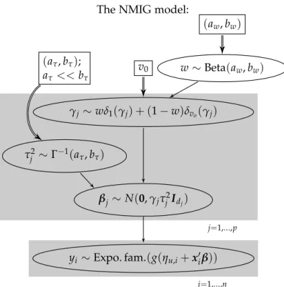
Figure 1 shows the hierarchy of the basic NMIG prior model. At the lowest level of the hierarchy, the datayi, i=1, . . . ,ncome from a distribution in the exponential family such as the Gaussian, binomial or poisson distributions. The canonical parameter of this distribution is connected to the linear pre-dictor via a known response function g(). The regression coefficients have

independent Gaussian priors with mean zero. Subvectors βj, j= 1, . . . ,pare associated with different components of the predictor, i.e. different covariates, unpenalized and penalized parts of a reparameterized spline basis or a set of indicator variables encoding the levels of a factor. The prior variance for β is constant within subvectors and given by the product of an indicator vari-able γj and the hypervariance τ_j2. The indicator variable γj takes the value 1 with probability w or some (very) small value v0 with probability 1−w.

The NMIG model: j=1,...,p i=1,...,n β_j ∼ N(0,γjτj2Idj) γj ∼ wδ1(γj) + (1−w)δvo(γj) w∼Beta(aw,bw) (aw,bw) v0 τ_j2∼Γ−1_(a τ,bτ) (aτ,bτ); aτ <<bτ yi ∼Expo. fam.(g(ηu,i+x0iβ))

Figure 1:Directed acyclic graph for the NMIG model.

Ellipses are stochastic nodes, rectangles are deterministic/logical nodes. Sin-gle arrows are stochastic edges, double arrows are logical/deterministic edges. Subvectorsβ_jare associated with different components of the

predic-tor, i.e. unpenalized and penalized parts of a reparameterized spline basis or indicators coding the different levels of a factor. djis the length of subvector

β_j. g()is a known response function. δy(x)is zero for any value ofx other

thanyand 1 aty. The linear predictor from model terms not associated with an NMIG prior is given byηu,i.

and scale parameterbτ with bτ aτ, so that the modebτ/aτ is significantly

greater than 1. The implied prior for the effective hypervariance v2

j = γjτj2 is a bimodal mixture of inverse gamma distributions, with one component strongly concentrated on very small values – thespikewithγj = v0and

effec-tive scale parameter v0bτ – and a second more diffuse component with most

mass on larger values – theslabwith γj = 1 and scale bτ. A coefficient

asso-ciated with a hypervariance that is primarily sampled from the spike-part of the prior will be strongly shrunk towards zero if v0 is sufficiently small, so

that the posterior probability forγj =v0can be interpreted as the probability

of exclusion of β_j from the model. The Beta prior for the mixture weights w

can be used to incorporate the analyst’s prior knowledge about the sparsity ofβor, more practically, enforce sufficiently sparse solutions for

overparame-terized models. In the following, we writeβ_j ∼NMIG(v0,w,aτ,bτ)to denote

this prior hierarchy for the regression coefficients.

Expressions for the full conditionals resulting from this prior structure are given in Section 4. This prior hierarchy is very well suited for selection of model terms for non-Gaussian data because the selection (i.e. the sampling of indicator variablesγ) occurs on the level of the hypervariances for the co-efficients. This means that the likelihood itself is not in the Markov blanket of γ and consequently does not occur in the full conditionals for the indi-cator variables. Since the full conditionals for γ are thus available in closed form regardless of the likelihood, this results in comparatively easy and fast model averaging for non-Gaussian models without the need to delve into the intricacies of estimating marginal likelihoods.

3.2 Using NMIG for simultaneous selection of multiple

coefficients fails

Previous approaches for Bayesian variable selection have primarily concen-trated on selection of single coefficients [George and McCulloch, 1993, Kuo and Mallick, 1998, Dellaportas et al., 2002, Ishwaran and Rao, 2005] or used very low dimensional bases for the representation of smooth effects. E.g. Cot-tet et al. [2008] use a pseudo-spline representation of their cubic smoothing spline bases with only 3 to 4 basis functions. In the following, we argue that conventional blockwise Gibbs sampling is ill suited for updating the state of the Markov chain when sampling from the posterior of an NMIG model even for moderately large coefficient blocks. We show that mixing for γj will be very slow for blocks of coefficients β_j with dj 1. We suppress the index j in the following.

The following analysis will show that, even if the blockwise sampler is ini-tially in an ideal state for switching between the spike and the slab parts of the prior, i.e. a parameter constellation so that the full conditional probabil-ity P(γ = 1|·) = .5, such a switch is very unlikely in subsequent iterations

for coefficient vectors with more than a few entries given the NMIG prior hierarchy.

con-∑

β₍2₁₎

∑

_β (0) 2 P

(

γ(1) = 1

)

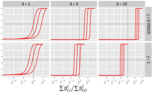
0.0 0.2 0.4 0.6 0.8 1.0 0.0 0.2 0.4 0.6 0.8 1.0 d=1 2−4 2−2 20 22 d=5 2−6 2−4 2−2 20 22 d=20 2−6 2−4 2−2 20 22 24 γ= 0.00025 γ= 1

Figure 2:P(γ)as a function of the relative change in∑dβ2for varyingd,γ₍₀₎: Inclusion probability in iteration (1) as a function of the ratio between the sum of squared coefficients in iteration (1) and (0). Lines in each panel correspond toτ₍2₁₎equal to the median of its full conditional and the .1- and .9-quantiles. Upper row is for γ₍₀₎ =1, lower row for γ₍₀₎ = v0. Columns correspond tod=1, 5, 20. Solid gray grid lines denote inclusion probability

=.5 and ratio of coefficient sum of squares=1

figuration ofat,bt,v0,w,τ₍2₀₎ andβ(0)so thatP(γ(0)=1|·) =.5. We setw=.5.

The parameters for whichP(γ=1|·) =.5 satisfy the following relations: P(γ=1|·) P(γ=v0|·) =v d/2 0 exp (1−v0) 2v0 ∑dβ2 τ2 ! =1, so thatP(γ=1|·)>.5 if ∑dβ2 dτ2 >− v0 1₋v0 log(v0), or

∑

d β2>−₁dv0 −v0 log(v0)τ 2_, orτ2>₋(1−v0)∑ d_β2 dv0log(v0) .

Assuming a given valueτ₍2₀₎, set d

∑

β2₍₀₎ = dv0

1−v0 log(v0)τ 2

(0).

Nowγ(0)takes on both valuesv0and 1 with equal probability, conditional on

In the following iteration, τ₍2₁₎ is drawn from its full conditional Γ−1(at+

d/2,bt+ ∑

d_β2

(0)

2γ(0) ) (see (7)). Figure 2 shows P(γ(1) = 1|τ 2

(1),∑dβ2(1)) as a

func-tion of ∑dβ2₍₁₎/∑dβ2₍₀₎ for various values of d. The 3 lines in each panel correspond to P(γ(1) = 1|τ(21),∑dβ2(1)) for values ofτ(21) equal to the median

of its full conditional as well as the .1- and .9-quantiles. The upper row in the Figure plots the function forγ(0) =1, the lower row forγ(0)=v0.

So, if we start in this “equilibrium state” we begin iteration (0)withv0,w, τ₍2₀₎, and β₍₀₎ so that P(γ(0) = 1|·) = .5. We then determine P(γ(1) =

1|τ₍2₁₎,∑dβ2₍₁₎)as a function of∑dβ2₍₁₎/∑dβ2₍₀₎ for

• various values of dim(β_j) =d,

• γ(0) =1 andγ(0)=v0,

• τ₍2₁₎at the .1, .5, .9-quantiles of its conditional distribution givenβ₍₀₎,γ(0).

The leftmost column in Figure 2 shows that moving betweenγ=1 andγ= v0 is easy for d = 1: For a large range of realistic values for∑dβ2₍₁₎/∑dβ2₍₀₎,

moving back to γ(1) = v0 from γ(0) = 1 (upper panel) has reasonably large

probability, just as moving from γ(0) = v0 to γ(1) = 1 (lower panel) is fairly

likely for realistic values of ∑dβ2₍₁₎/∑dβ2₍₀₎. For d = 5, however, P(γ(1) =

1|·)already resembles a step function. For d = 20, if ∑dβ2₍₁₎/∑dβ2₍₀₎ is not smaller than 0.48, the probability of moving fromγ(0) =1 toγ(1) =v0(upper

panel) is practically zero for 90% of the values drawn fromp(τ₍2₁₎|·). However, draws of β that reduce ∑dβ2 by more than a factor of 0.48 while γ = 1 are unlikely to occur in real data. It is also extremely unlikely to move back to γ(1) = 1 when γ(0) = v0, unless ∑dβ2₍₁₎/∑dβ2₍₀₎ is larger than 2.9. Since

the full conditional for β is very concentrated if γ = v0, such moves are

highly improbable and correspondingly the sampler is unlikely to move away from γ = v0. Numerical values for the graphs in Figure 2 were computed

for aτ = 5, bτ = 50, v0 = 0.005 but similar problems arise for all suitable

hyperparameter configurations.

In summary, mixing of the indicator variablesγwill be very slow for long subvectors. In experiments, we observed posterior means of P(γ = 1) to be

either_≈0 or _≈1 across a wide variety of settings, even for very long chains, largely depending on the starting values of the chains. The following section describes a possible remedy.

3.3 Parameter Expansion: The peNMIG Model

The mixing problem analyzed in the previous section is similar to the mix-ing problems encountered in other samplers for hypervariances of regression coefficients: a small variance for a batch of coefficients implies small coeffi-cient values and small coefficoeffi-cient values in turn imply a small variance so that the sampler is unlikely to exit a basin of attraction around the origin. This

problem has been previously described in Gelman et al. [2008], where the issue is framed as one of strong dependence between a block of coefficients and their associated hypervariance. A bimodal prior for the variance such as the NMIG prior where the Markov chain must switch between the different components of the mixture prior associated with the two modes of course ex-acerbates these difficulties. A promising strategy to reduce this dependence is the introduction of working parameters that are only partially identifiable along the lines of parameter expansionor marginal augmentationintroduced for the EM-algorithm in Meng and van Dyk [1997] and developed further for Bayesian inference for hierarchical models in Gelman et al. [2008]. While Gel-man et al. [2008] concentrate on speeding up convergence for conventional hierarchical models, we use the parameter expansion to enable simultaneous selection or deselection of coefficient subvectors and improve the shrinkage properties of the resulting marginal prior.

We add a redundant multiplicative parameterization to the spike-and-slab prior. We set

β_j =αjξj; ξj ∈Rdj

for a subvector β_j with lengthdj and use a scalar parameter

αj ∼NMIG(v0,w,aτ,bτ),

where NMIG denotes the prior hierarchy given in Fig. 1. Entries of the vector

ξ_j are a priori distributed as

ξjk i.i.d.∼ 1₂N(1, 1) +1₂N(−1, 1), k=1, . . . ,dj,

and prior independence betweenαj andξj. We write

β_j ∼peNMIG(v0,w,aτ,bτ)

as shorthand for this prior structure.

The effective dimension of the coefficient vector associated with updating γj andτ_j2 is then equal to one in every penalization group, since the Markov blankets of bothγjandτjnow only contain the scalar parameterαjinstead of the vectorβ_j. This is crucial in order to avoid the mixing problems described

in the previous Section, because instead of

P(γ=1|·) P(γ=v0|·) =v d/2 0 exp (1₂−_vv0) 0 ∑di β2i τ2 !

for the conventional NMIG prior, we now have

P(γ=1|·) P(γ=v0|·) = √_v 0exp (1−v0) 2v0 α2 τ2 ,

which is less susceptible to result in extreme values and behaves more like the probabilities in the leftmost column of Figure 2.

In our parameter expansion, the parameter αj parameterizes the “impor-tance” of the j-th coefficient block, while ξ_j “distributes”αj across the entries in β_j. Setting E(ξ) = _±1 shrinksξ towards |1|, the multiplicative identity, so that the interpretation of αj as the “importance” of the j-th coefficient block can be maintained and yields a marginal prior forβ_j that is less concentrated

on small absolute values thanξ ∼ N(0, 1).

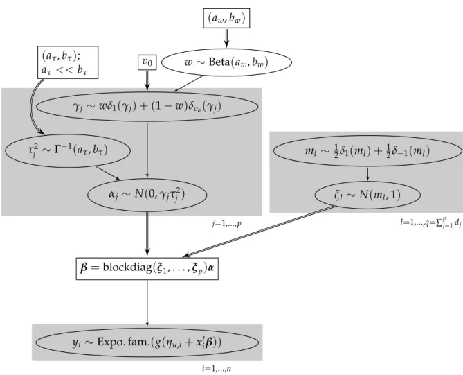
peNMIG: NMIG with parameter expansion

j=1,...,p l=1,...,q=∑pj=1dj i=1,...,n αj ∼ N(0,γjτj2) γj ∼wδ1(γj) + (1−w)δvo(γj) v0 w∼Beta(aw,bw) (aw,bw) τ_j2 ∼Γ−1_(a τ,bτ) (aτ,bτ); aτ <<bτ ξl ∼ N(ml, 1) ml ∼ 1₂δ1(ml) + 1₂δ−1(ml) β=blockdiag(ξ₁, . . . ,ξ_p)α yi ∼Expo. fam.(g(ηu,i+x_i0β))

Figure 3:Directed acyclic graph of NMIG model with parameter expansion. Ellipses are stochastic nodes, rectangles are deterministic/logical nodes. Sin-gle arrows are stochastic edges, double arrows are logical/deterministic edges.

Figure 3 shows the prior hierarchy for the model with parameter expansion. In the following, this model will be denoted as peNMIG. The vector ξ = (ξ0₁, . . . ,ξ_p)0 is decomposed into subvectors ξ_j associated with the different

3.4 Shrinkage properties

Marginal priors

This section investigates the regularization properties of the marginal prior for the regression coefficients β implied by the hierarchical prior structures

given in Figs. 1 and 3. To distinguish between the conventional NMIG prior and its parameter expanded version we writeβif the parameter has an NMIG prior and βpe if it has the parameter expanded peNMIG prior. In the follow-ing, we analyze the univariate marginal priors

p(β|aτ,bτ,aw,bw,v0) =

=

Z

p(β|γ,τ2)p(τ2|aτ,bτ)p(γ|w,v0)p(w|aw,bw)dτ2dγdw for the conventional NMIG model and

p(βpe=αξ|aτ,bτ,aw,bw,v0) = Z p(α|γ,τ2)p βpe α | {z } =ξ 1 |α|p(τ 2_|a τ,bτ)p(γ|aw,bw,v0) p(w|aw,bw)dαdτ2dγdw

for the peNMIG prior.

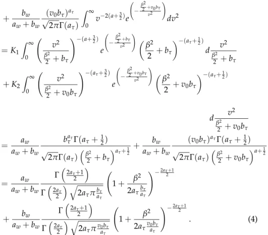
These are the univariate marginal priors for a single regression coefficient with and without parameter expansion with the intermediate quantitiesτ2,γ and w integrated out. We analyze the marginal priors because it has been shown that the shrinkage properties of the resulting posterior means are de-pendent on their shape and less on that of the conditional priors [Fahrmeir et al., 2010, Kneib et al., 2010]. We use v2 _{= γτ}2 _{∼ Γ}−1_(a

τ,γbτ) so that the

marginal prior for β in the conventional NMIG-model is a mixture of scaled t-distributions with 2aτ degrees of freedom and scale factors √v0bτ/aτ and

√

bτ/aτ with weights _awb+wbw and

aw aw+bw, respectively: p(β|aτ,bτ,aw,bw,v0) = = aw aw+bw Z _∞ 0 p(β|v 2_)p(v2_|a τ,bτ)dv2 + bw aw+bw Z _∞ 0 p(β|v 2_)p(v2_|a τ,v0bτ)dv2 = aw aw+bw baτ τ √ 2πΓ(aτ) Z _∞ 0 v −2(a+3₂)_e − β2 2+bτ v2 ! dv2

+ bw aw+bw (v0bτ)aτ √ 2πΓ(aτ) Z ∞ 0 v −2(a+3₂)_e − β2 2 +v₀bτ v2 ! dv2 =K1 Z _∞ 0 v2 β2 2 +bτ !₋(a+3₂) e − β2 2 +bτ v2 ! β2 2 +bτ −(aτ+1₂) d v2 β2 2 +bτ +K2 Z _∞ 0 v2 β2 2 +v0bτ !−(aτ+3₂) e − β2 2 +v0bτ v2 ! β2 2 +v0bτ −(aτ+12) d v2 β2 2 +v0bτ = aw aw+bw baτ τ Γ(aτ+ 1₂) √ 2πΓ(aτ) β2 2 +bτ aτ+12 + bw aw+bw (v0bτ)aτΓ(aτ+ 1₂) √ 2πΓ(aτ) β2 2 +v0bτ a+1₂ = aw aw+bw Γ2aτ+1 2 Γ2aτ 2 q 2aτπb_aτ_τ 1+ β2 2aτb_aτ_τ !₋2aτ+1 2 + bw aw+bw Γ2aτ+1 2 Γ2aτ 2 q 2aτπv0_ab_ττ 1+ β2 2aτv0b_aττ !₋2aτ+1 2 . (4)

The marginal prior for βpe in the peNMIG model has no closed form. The density given in (4) is also the marginal priorp(α|aτ,bτ,aw,bw,v0)forαin the

peNMIG model so that a density transform yields

p(βpe=αξ|aτ,bτ,aw,bw,v0) = = Z p(α|aτ,bτ,aw,bw,v0)p βpe α | {z } =ξ 1 |α|dα = Z p βpe ξ |aτ,bτ,aw,bw,v0 p(ξ) 1 |ξ|dξ. (5)

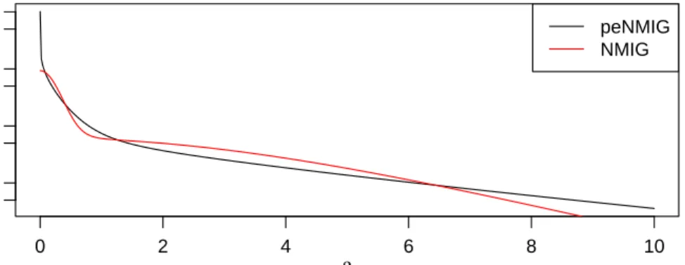
Figure 4 shows the two marginal priors for v0 = 0.005, (aτ,bτ) = (5, 50)

andaw=bw. Values for peNMIG were determined by numerical integration. Note the characteristic shape of the spike-and-slab prior for the marginal prior without parameter expansion: There is a “spike” around zero which corre-sponds to the contribution of the t-distribution with scale factor √v0bτ/aτ

and a “slab” which corresponds to the contribution of the t-distribution with scale factor √bτ/aτ. The prior for peNMIG has heavier tails and an infinite

spike at zero (see (6)). It looks similar to the original spike-and-slab prior sug-gested by Mitchell and Beauchamp [1988], which used a mixture of a point mass in 0 and a uniform distribution on a finite interval, but sampling for our approach has the benefit of conjugate and proper priors.

0 2 4 6 8 10 5e−03 1e−01 5e+00 β p ( β ) peNMIG NMIG

Figure 4:Marginal priors forβas given in (4) and (5) with(aτ,bτ) = (5, 50),

v0=0.005,aw =bw. (Log scale on vertical axis.)

The following shows that the marginal prior p(βpe)diverges in 0. We use

p(βpe|aτ,bτ,aw,bw,v0) = Z +∞ −∞ pα _β pe ξ pξ(ξ) 1 |ξ|dξ, so that p(βpe|aτ,bτ,aw,bw,v0)|βpe=0 = pα(0) Z +∞ −∞ pξ(ξ) 1 |ξ|dξ.

It is enough to show that I = R₋+_∞∞pξ(ξ)_|1_ξ|dξ diverges, since pα(0) is finite

and strictly positive. The prior pξ() is a mixture of normal densities with

variance 1 and means_±1, so

I =KZ +∞ −∞ 1 |ξ| exp −(ξ+₂1)2 +exp −(ξ−₂1)2 dξ =K(I1+I2+I3+I4) with I1= Z 0 −∞− 1 ξ exp −(ξ+₂1)2 dξ, I2= Z +∞ 0 1 ξ exp −(ξ+₂1)2 dξ, I3= Z ₀ −∞− 1 ξ exp −(ξ−₂1)2 dξ, and I4= Z +∞ 0 1 ξ exp −(ξ−₂1)2 dξ. Note that I1= I4andI2= I3. Since all 4 integrals are positive, it is enough to

show that one of them diverges:

I4= Z ₁ 0 1 ξexp −(ξ−₂1)2 | {z } ≥e−1_{2 forξ∈[0,1]} dξ+ Z +∞ 1 1 ξ exp −(ξ−₂1)2 dξ | {z } =K˜≥0

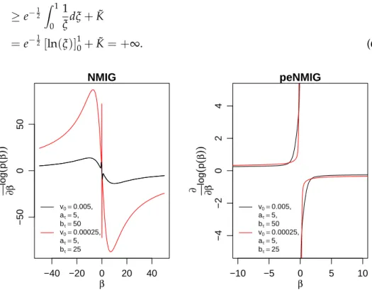
≥e−12 Z ₁ 0 1 ξdξ+K˜ =e−12 _[ln_(ξ)]1₀₊K˜ _{= +}∞. (6) −40 −20 0 20 40 −50 0 50 NMIG β ∂ log _∂β ( p ( β )) v0=0.005, aτ=5, bτ=50 v0=0.00025, aτ=5, bτ=25 −10 −5 0 5 10 −4 −2 0 2 4 peNMIG β ∂ log _∂β ( p ( β )) v0=0.005, aτ=5, bτ=50 v0=0.00025, aτ=5, bτ=25

Figure 5:Score functions for marginal priors for beta as given in (4) and (5). Note the different scales for the conventional NMIG and peNMIG.

For both NMIG and peNMIG, the tails of the marginal priors are heavy enough so that they have redescending score functions (see fig. 5) which ensures Bayesian robustness of the resulting estimators. While the shape of peNMIG’s score function is similar to that of an _Lq-prior with q → 0 and is fairly robust towards different combinations of hyperparameters, the con-ventional NMIG score function has a complicated shape determined by the interaction ofaτ,bτ andv0. Note that the score function of the marginal prior

under parameter expansion descends monotonously and much faster.

The marginal prior of the hypervariances for βpe = αξ is given by the density of the product γτ2ξ2 since βpe|γ,τ2,ξ ∼ N(0,γτ2ξ2). This marginal prior, which is the integral over the product of a mixture of scaled inverse gamma distributions with a noncentralχ2₁distribution

p(λ2 =γτ2ξ2) = = Z _∞ 0 aw aw+bwΓ −1λ2 ξ2|aτ,bτ + bw aw+bwΓ −1λ2 ξ2|aτ,v0bτ 1 ξ2χ 2 1(ξ2|µ=1)dξ2, Γ−1_{(x|a,b) =} ab Γ(a)x− (a+1)_exp −b_x , χ2₁(x|µ=1) = 1 2exp −x+₂ 1 x−14I −12 √ x,

(Iν(y) denotes the modified Bessel function of the first kind) is intractable,

so we are unable to verify whether conditions for Theorem 1 in Polson and Scott [2010] apply. Simulation results indicate that the peNMIG prior has similar robustness for large coefficient values and better sparsity recovery as the horseshoe prior (see p. 30), for which the theorem applies.

The peNMIG prior combines an infinite spike at zero with heavy tails. This desirable combination is similar to other shrinkage priors such as the horseshoe prior [Carvalho et al., 2010] and the normal-Jeffreys prior [Bae and Mallick, 2004] for which both robustness for large values of β and very effi-cient estimation of sparse coeffieffi-cient vectors have been shown [Carvalho et al., 2010, Polson and Scott, 2010].

Constraint regions

The shapes of the 2-d constraint regions logp((β1,β2)0) ≤ const implied by

the NMIG and peNMIG priors provide some further intuition about their shrinkage properties. The contours of the NMIG prior, depicted on the left

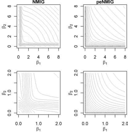
Figure 6:Contour plots of logp((β1,β2)0) for aτ = 5, bτ = 50,v0 = 0.005,

aw =bwfor the standard NMIG model and the model with parameter

expan-sion. Lower panels are zooms into the region around the origin (indicated in the upper panels).

in fig. 6, have different shapes depending on the distance from the origin. Close to the origin (β < .3), they are circular and very closely spaced,

im-plying strong ridge-type shrinkage – coefficient values this small fall into the “spike”-part of the prior and will be strongly shrunk towards zero. Moving away from the origin (.3 < β < .8), the shape of the contours defining the constraint region morphs into a rhombus shape with rounded corners that is similar to that produced by a Cauchy prior. Still further from the origin (1 < β < 2), the contours become convex and resemble those of the con-tours of an Lq penalty function, i.e. a prior with p(β) ∝ exp(−|β|q), with

q<1. Coefficient pairs in this region will be shrunk towards one of the axes, depending on their posterior correlation and which of their maximum like-lihood estimators is bigger. For even larger β, the shape of the contours is a mixture of a ridge-type circular shape around the bisecting angle with pointy ends close to the axes. The concave shape of the contours in the areas far from the axes implies proportional (i.e. ridge-type) shrinkage of very large coeffi-cient pairs. This corresponds to the comparatively smaller tail robustness of the conventional NMIG prior observed in simulations.

The shape of the constraint region implied by the peNMIG prior has the convex shape of a Lq-penalty function with q < 1, which has the desirable properties of simultaneous strong shrinkage of small coefficients and weak shrinkage of large coefficients due to its closeness to theL0 penalty (see also

fig. 8).

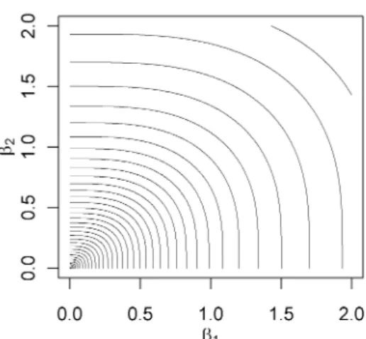
Until now, the discussion has been limited to bivariate shrinkage proper-ties applied to single coefficients from separate penalization groups. In the following, we discuss shrinkage properties for coefficients from thesame pe-nalization group, i.e. two entries from the same subvector β_j in the

nota-tion of Figs. 1 and 3. The shape of the peNMIG prior for 2 coefficients from the same penalization group is quite different. Recall that two co-efficients (β1,β2) from the same penalization group share the same α, e.g.

in this case (β1,β2)0 = α(ξ1,ξ2)0. This results in a very different shape of

logp((β1,β2)0) ≤ const shown in Figure 7 (values determined by numerical

integration). The prior in this case is

p(β_pe =α(ξ1,ξ2)0|aτ,bτ,aw,bw,v0) = = Z p(α|aτ,bτ,aw,bw,v0)p β_pe α ! 1 |α|dα = Z p(α|aτ,bτ,aw,bw,v0) 1 |α|· ·1₄ N β1 α |µ=1 +N β1 α |µ= −1 · · N β2 α |µ=1 +N β2 α|µ=−1 dα,

where N(x|µ)denotes the normal density with variance 1 and mean µ. The shape of the constraint region for grouped coefficients is that of a square with rounded corners. Compared with the convex shape of the constraint region, this shape induces less shrinkage toward the axes and more towards the origin or along the bisecting angle.

Figure 7: Constraint region for β = (β1,β2)0 from the same penalization group.

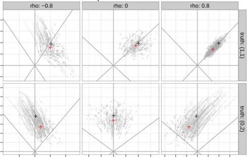
Figure 8 illustrates the difference in shrinkage behavior between grouped and ungrouped coefficients for a simple toy example. We simulated design matrices X with n = 15 observations and 2 covariates so that (X0_X)−1 _{= 1ρ}

ρ1

with ρ =−0.8, 0, 0.8. Coefficients βwere either(1, 1)0 (two

intermedi-ate effect sizes) or(0, 2)0 (one null, one large effect) and observations y were

generated with a signal-to-noise ratio of 2. We generated 100 datasets for each combinations ofρandβand compared OLS estimates to the posterior means

for a peNMIG model as returned byspikeSlabGAM.

The different shrinkage properties for grouped and ungrouped coefficients are most apparent for uncorrelated coefficients (middle column): Shrinkage in this case occurs in directions orthogonal to the contours of the prior, so while the shape of the grouped prior causes shrinkage toward the origin in the direction of the bisecting angle or parallel to the axes, the ungrouped coefficients are shrunk more toward the nearest axis. Consequently, we expect estimation error for sparse coefficient vectors with few large and many small or zero entries (likeβ= (0, 2)0_{) to be smaller for ungrouped coefficients, while} the grouped prior should have a smaller bias for coefficient vectors with many entries of similar (absolute) size (like β= (1, 1)0): While most of the mass of

the multivariate prior for ungrouped coefficients is concentrated along the axes (i.e. on sparse coefficient vectors), the multivariate prior for grouped coefficients is concentrated in a cube around the origin.

Grouped coefficients β1 β2 −0.5 0.0 0.5 1.0 1.5 2.0 0.0 0.5 1.0 1.5 2.0 2.5 3.0 3.5 rho: −0.8 −1 0 1 2 rho: 0 −1.0 −0.5 0.0 0.5 1.0 1.5 rho: 0.8 −1.5 −1.0 −0.5 0.0 0.5 1.0 1.5 tr uth: (1,1) tr uth: (0,2) Single coefficients β1 β2 −0.5 0.0 0.5 1.0 1.5 2.0 0.0 0.5 1.0 1.5 2.0 2.5 3.0 3.5 rho: −0.8 −1 0 1 2 rho: 0 −1.0 −0.5 0.0 0.5 1.0 1.5 rho: 0.8 −1.5 −1.0 −0.5 0.0 0.5 1.0 1.5 tr uth: (1,1) tr uth: (0,2)

Figure 8: Shrinkage for grouped (top graph) and ungrouped coefficients (bottom graph).

Arrows connect OLS estimates with posterior means fromspikeSlabGAMon identical data sets. Black crosses denote means of OLS estimators over all replications for a given setting, red crosses means of posterior means from a peNMIG model fit withspikeSlabGAM. Top rows in each graph are for β = (1, 1)0, bottom rows for β = (0, 2)0. Columns show results for

ρ =−0.8, 0, 0.8. Note thatρis the correlation of the OLS estimators, not the correlation of the associated covariates.

4 MCMC

This section describes the MCMC sampler implemented inspikeSlabGAMthat was used for all the simulations and applications in Sections 5 and 6. Algo-rithm 1 on p. 26 gives a short summary of the blockwise Metropolis-within-Gibbs sampler we use.

4.1 Full conditionals

The sampler exploits the fact that the full conditionals of (most of) the param-eters are available in closed form:

w|· ∼Beta aw+ p

∑

j δ1(γj),bw+ p

∑

j δv0(γj) ! , τ_j2|· ∼Γ−1  at+dj/2,bt+ ∑ dj i=1β2ji 2γj  , P(γj =1|·) P(γj =v0|·) =v dj/2 0 exp  (1−v0) 2v0 ∑dj i=1β2ji τ_j2  . (7)

Full conditionals for β_j for Gaussian responses and the conventional NMIG

model (given in fig. 1) are given by

β_j|· ∼N(µ_j,Σj) (8) with Σj = 1 σε2 X0 jXj+ 1 γjτ_j2Idj !₋1 ; µ_j = 1 σε2 ΣjX0jy.

In the peNMIG model given in fig. 3, updates for α use the “collapsed”

design matrix Xα = Xblockdiag(ξ₁, . . . ,ξ_p), while ξ is updated based on a

“rescaled” design matrixXξ =Xblockdiag(1d1, . . . ,1d p)α, where1d is ad×1 vector of ones. For Gaussian responses, these are draws from their multi-variate normal full conditionals as above. For non-Gaussian responses, we use P-IWLS proposals [Lang and Brezger, 2004] with a Metropolis-Hastings step. The following Section 4.2 provides more details on the methods used to sampleβ.

Note that

P(γj =1|·)

P(γj =v0|·) >v

dj/2

0 for all values ofβj, i.e that

P(γj =1|·)> v dj/2 0 1+vd₀j/2 ≈v dj/2 0 for smallv0.

4.2 Updating

β

_pe

This section describes the implementation of the updates for the regression coefficients in the peNMIG model. For both Gaussian and non-Gaussian re-sponses, the proposed algorithm does blockwise updates of coefficient sub-vectors, conditional on the remainder of the coefficient vector and the other parameters in the Markov blanket (i.e. prior covariances, prior means and the relevant likelihood terms). The default is a blocksize of 30 for bothαandξ for

Gaussian response and smaller blocksizes of 5 and 15 forαandξ, respectively,

for non-Gaussian response. Blocksizes are smaller for non-Gaussian response since the acceptance probability in the necessary Metropolis-Hastings-step for non-Gaussian responses tends to decrease quickly with increasing dimension of the proposal.

Sinceβ=blockdiag(ξ₁, . . . ,ξ_p)α, we sampleβby first updatingαbased on

a “collapsed”n×pdesign matrixXα =Xblockdiag(ξ₁, . . . ,ξ_p)and then

up-datingξbased on a “rescaled”n×qdesign matrixXξ =Xblockdiag(1d1, . . . ,1d p)α, where 1_d is a d_×1 vector of ones. The j-th column of Xα contains the sum

of the original design columns multiplied by the entries in the subvector ξ_j

associated with αj. Each column in Xξ contains the respective column of

the original design matrix multiplied by the associated entry in α. The prior

means ml ∈ {±1} for ξl ∼ N(ml, 1) are drawn beforehand from their full conditionals viaP(ml =1|·) = ₁+exp1(₋2ξl).

Update via QR-decomposition

The following paragraphs describe a general method to update a coefficient vector δassociated with a conditional Gaussian prior. We use this procedure

to update βin the NMIG model and to update both αandξ in the peNMIG

model.

Regression coefficients δ with prior δ ∼ N(µδ,Σδ) and associated design

matrix Xδ _{can be updated by running the regression of an augmented data}

vectory˜ with covarianceΣe on an augmented design matrixX˜ with

˜ y = y µδ ; Xe = Xδ I andΣe = Cov(y) 0 0 Σδ . (9)

If only a subvector δj is updated conditional on the remainder δ−j of the vectorδ,yis replaced byy−Xδ

−jδ−j andΣδ is replaced byΣδ−j,−j.

Following Gelman et al. [2008], we perform the updates for the regression coefficients via the QR-decomposition Σe−1/2X˜ = QR. From this decomposi-tion, we can solve the triangular system Rδˆ = QΣe−1/2y˜ for the mean of the full conditional δˆ. As long as Σe−1/2 is a diagonal matrix, as is the case for all of the models and predictor terms we are considering (see Section 2.3), or is known, the computationally demanding step is the computation of the QR-decomposition.

We solve another triangular system Reδ = n, ni i.i.d.∼ N(0, 1) in order to

generate a candidate value δc = δˆ+eδ from (the approximation to) the full

conditional, so the proposal distributionq(δc,δ)is N(δˆ,(R0R)−1).

IWLS updates for non-Gaussian responses

We use a variant of the well-known IWLS proposal scheme [Gamerman, 1997] to do blockwise updates for bothα and ξ in the non-Gaussian case. We use

a penalized IWLS (P-IWLS) proposal scheme based on an approximation of the current posterior mode described in detail in Brezger and Lang [2006] (Sampling scheme 1, Section 3.1.1). This method is a Metropolis-Hastings type update which uses a Gaussian (i.e. second order Taylor) approximation to the full conditional around its approximate mode as its proposal distribu-tion. The approximating Gaussian is obtained by performing a single Fisher scoring step per iteration.

For P-IWLS, y and Cov(y) in (9) are replaced by their IWLS equivalents [Gamerman, 1997]

Cov(y)IWLS_≈ diag b00_(θ)g0_(µ)2 _andy IWLS_{≈ X}

jδj+ (y−µ)g0(µ), (10)

see (1) for notation.

We use the following modification of the IWLS-algorithm in order to de-crease the computational complexity of the algorithm somewhat: By using the mean of the proposal distribution of the previous iteration δˆp instead of δin (10) and recalculatingµ andθbased onδˆp, the proposal distributionq()

becomes independent of the current state, which simplifies the calculation of the acceptance probability and can increase acceptance rates [Brezger and Lang, 2006].

Acceptance rates for the sampler strongly depend on the size of the update blocks and on the magnitude of the rescaling performed in each iteration: For large blocks or updates that require drastic rescaling (see paragraph be-low), acceptance probabilities can occasionally become small, especially for binary responses. To avoid getting stuck, our sampler monitors rejection rates for each block. If proposals for a certain update block have been re-jected 10 times in a row, we use a different proposal density for this block with probability 0.5: Instead of drawing proposals from N(δˆp,(R0R)−1), we

useq(δc,δ) =N(δc,(R0R)−1), i.e. we use the current state as the mean of the

proposal. The working observations and IWLS weights that determineRare calculated from the mode of the previous iteration as described above so that the proposal ratioq(δ,δc)/q(δc,δ)is 1. This type of update tends to result in

smaller steps, but it is useful in order to get the chain moving again. Using an adaptive transition kernel such as this one can violate the detailed balance condition for the transition kernel of the Markov chain, but results in Section 5 convincingly show that convergence of the chains is not adversely affected. For most datasets, mode switching occurs very rarely during the sampling of the chain if at all, and spikeSlabGAM provides the option to switch it off

entirely. Direct comparisons of results on problematic datasets between ex-ceedingly long (i.e. > 100000 iterations for a model with 20 coefficients) runs of single-site-IWLS-updates without mode switching and blocked updates with mode switching showed that differences between the resulting posterior distributions were well within the range of MC error.

Rescaling parameter blocks

After updating the entire α− and ξ−vectors, each subvector ξ_j is rescaled

so that |ξ_j|has mean 1, and the associated αj is rescaled accordingly so that

β_j =αjξj is unchanged: ξ_j → dj ∑d_ij|ξji| ξ_j and αj → ∑ dj i |ξji| dj αj.

This rescaling is advantageous since αj and ξj are not identifiable and thus their sampling paths can wander off into extreme regions of the parameter space without affecting the fit, e.g. αj becoming extremely large while en-tries in ξ_j simultaneously become extremely small. By rescaling, we retain

the interpretation ofαj as a scaling factor representing the importance of the model term associated with it and avoid numerical problems that can oc-cur for extreme parameter values. For non-Gaussian responses, the posterior modes used in the IWLS-updates are shifted accordingly as well. Note, how-ever, that this shifting of the mode is only approximate. Consequentially, this rescaling can occasionally lead to low (<.1) acceptance rates for the P-IWLS proposals since the proposal density may not be well adapted to the posterior anymore after a large rescaling.

Starting values

It is essential to find suitable starting values forβfor non-Gaussian responses,

otherwise the IWLS sampler fails. We initialize βby performing Fisher

scor-ing steps with fixed and usually large values of the hypervariance until the relative change in β are smaller than 10%, up to a maximum of 20 steps.

Starting values forα(0) andξ(0) are computed via

α(_j0)= ∑ dj i |βji| dj and ξ (0) j = β_j α(_j0).

Simulation results and applications (Sections 5, 6) show that this strategy works well.

4.3 Estimating Inclusion Probabilities

Selection of coefficient blocks β_j in the NMIG and peNMIG models is based

Algorithm 1MCMC sampler for peNMIG

1: Initialize τ2(0),γ(0),σ2(0),w(0) and β(0) (via IWLS for non-Gaussian

re-sponse as described on p. 25) 2: Computeα(0),ξ(0),X(α0)

3: foriterationst =1, . . . ,Tdo

4: forblocksb=1, . . . ,Bα do

5: generateα(_bt) from its full conditional (Gaussian case)/ via IWLS-P

6: X(_ξt) =Xblockdiag(1d1, . . . ,1dp)α(t)

7: generatem(₁t), ...,m(qt) from their full conditionals 8: forblocksb=1, . . . ,Bξ do

9: generateξ(_bt) from its full conditional (Gaussian case)/ via IWLS-P

10: forpenalization groupsi=1, . . . ,p do 11: rescaleξ(_it)andα(_it) (see p. 25) 12: X(αt) =Xblockdiag(ξ₁(t), . . . ,ξ(_pt))

13: generateτ12(t), ...,τp2(t) from their full conditionals 14: generateγ1(t), ...,γp2(t)from their full conditionals 15: generatew(t)_{from its full conditional}

16: ifyis Gaussianthen

17: generateσ2(t)from its full conditional

posterior inclusion probability pin,j, since pin,j = P(γj = 1) = E(δ1(γj)). In-clusion probabilities pin,j are estimated with the Rao-Blackwellized estimator

d pin,j =T−1 T

∑

t=0 p(_int)_,j , with p(_int)_,j =1−            1+vdj/2 0 exp (12−v0v0 ) ∑dji=1(β(jit))2 (τ_j2)(t) !!₋1 for NMIG, 1+v1/2₀ exp (1−v0) 2v0 (α(_jt))2 (τ_j2)(t) −1 for peNMIG, whereθ(t)denotes the realized value of parameterθin iterationtof an MCMC chain with length T. This estimator uses the MCMC samples of P(γj = 1) after burn-in, instead ofpdin,j =T−1∑tT=0δ1(γ(_jt)).

Barbieri and Berger [2004] show that, under fairly strong conditions, the

median probability model, i.e. the model which includes only covariates with a marginal inclusion probability greater than 0.5, is optimal for predictive pur-poses in the class of single models. Although the conditions set forth (i.e. orthogonal design, squared error loss) do not apply to most of the settings in whichspikeSlabGAMcould conceivably be used, we still use this threshold of

pin,j = 0.5 to determine exclusion or inclusion of model terms in the follow-ing. We concur with their assertion that “[. . .] the fact that onlythe median

that it might quite generally be successful, even when the optimality theory does not apply” [Barbieri and Berger, 2004, p. 894] and this is borne out by simulation studies and applications (see Sections 5, 6).

4.4 Algorithm Variants

While the default prior for the inclusion indicators γj assumes mutual dependence, i.e. that inclusion or exclusion of a model term is a priori in-dependent of the inclusion or exclusion of all other model terms, we also implemented a structure of the prior for γ that incorporates the hierarchical

structure of the model terms themselves. More precisely, the prior structure forces inclusion of e.g. the linear term for a covariate if the corresponding smooth term is included in the model, or the inclusion of main effects if an interaction effect involving them is included in the model. Without changing the sampler per se, this “top-down” approach is implemented as a simple pass over the updated γ-vector in each iteration, making sure that all

low-order terms (i.e. main effects) have γ = 1 if high-order terms that involve

them (i.e. interactions) haveγ = 1. Alternatively, a “bottom-up” variant en-forcing more parsimonious models that excludes high-order terms (i.e. sets them toγ= v0) unless all low-order terms associated with them are included

may be an option worth pursuing, but we have not done so yet. An alterna-tive to be implemented in future versions of the software is to sample γ not

via single-site updates, but blockwise with blocks determined by the depen-dencies induced by the hierarchy (e.g. sample γs for main effects and their interaction together) and then include a Metropolis-Hastings step to reject proposals that violate the hierarchical constraints in a block.

5 Simulation Studies

The following sections summarize results from tests of the proposed meth-ods on simulated data. Section 5.1 investigates the adaptive shrinkage prop-erties of the proposed prior. Section 5.2 shows that the proposed parameter expansion with multiplicative redundant parameters can improve sampling behavior for settings in which the posterior of the regression coefficients con-tains strong correlations. Sections 5.3 and 5.4 investigate model selection and estimation performance for models with random intercepts and smooth func-tions, respectively. Section 5.5 describes results for additive models of some complexity for both Gaussian and Poisson responses and compares the per-formance of our approach to the perper-formances of other recently suggested algorithms.

We introduce some additional notation for the generation of Gaussian data: For a given data-generating process (DGP) that generates a random design matrixX and a (fixed or random) vector of coefficients β, let η= Xβdenote

the “true” linear predictor. For responses withy = η+ε, the difficulty level

of estimating both β, and, consequently, η is determined mostly by the

variability ofη, i.e. the “signal”, and the unsystematic variability introduced

by the Gaussian error termse, the “noise”. Let sdη =

p

∑n_i(ηi−η¯)2/n and define the signal-to-noise ratio SNR=nsd2_η/∑n_i ε2_i. For a given value of SNR and realization ofη, responsesyare then generated viayi ∼ N

ηi, sd2η/ SNR

.

5.1 Adaptive shrinkage

We investigate the shrinkage properties of the proposed prior structures in a simple setting. The following describes the data-generating process:

• n=20, 50, 100 observations • β= (.1, .2, .3, . . . , 1),p=10 • signal-to-noise ratio SNR=0.5, 2

• covariates xj are independent, with xj ∼ U[−2, 2] and enter the model scaled to have mean 0 and standard deviation .5.

• 100 replications per setting

We compare the shrinkage properties of the posterior means fromspikeSlabGAM

with those of the horseshoe prior (HS) as implemented in R packagemonomvn

[Gramacy, 2010] and the LASSO estimator (L1) as implemented in R package

lasso2[Lokhorst et al., 2009]. The horseshoe prior (a scale mixture of normals with a scaled half-Cauchy mixing distribution, where the scale of the mix-ing distribution is itself half-Cauchy distributed), has recently been shown to have excellent adaptive shrinkage properties [Carvalho et al., 2010] and we use its behavior as a reference for good adaptive shrinkage properties, while the LASSO estimators serve as a reference for a shrinkage estimator without adaptivity.

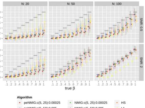
Figure 9 shows the median and the inter-quartile ranges of the posterior means of the estimated coefficients over the 100 replications for each combina-tion of the different numbers of observacombina-tionsn and the signal-to-noise ratios SNR. We compare models with (peNMIG) and without (NMIG) the redun-dant multiplicative parameter expansion with(aτ,bτ,v0) = (5, 25, 0.00025)or (5, 50, 0.005).

Note that the frequentist LASSO (L1, in yellow) performs about the same amount of regularization in all of the settings – all six approaches overshrink the larger coefficients for N=20 andN =50, SNR=0.5; LASSO less so than

the Bayesian approaches. However, as more information from the data be-comes available with increasingNand SNR, the Bayesian approaches (NMIG, peNMIG, HS) perform less regularization, since the likelihood contribution of the posterior increasingly dominates the prior contribution to the poste-rior. This is visible especially for the bottom right panel with N = 100 and

SNR=2.

Adaptive shrinkage in the sense of strong regularization of smaller coeffi-cients (i.e. β≤ 0.5) and simultaneously weak shrinkage for large coefficients

true β β ^ 0.0 0.2 0.4 0.6 0.8 1.0 0.0 0.2 0.4 0.6 0.8 1.0 N: 20 ●●●●●●●●●●● ●●●●●●●● ●_●●● ●● ● ●●●●●●●●●●● ● ●● ● ● ●●●● ● ● ● ● ●●● ● ● ● ●● ● ● ●●●●● ●●●●●● ●● ● ●● ● ●● ● ●● ● ●● ● ●● ● ● ● ● ● ●● ● ● ● ● ● ● ● ● ● ● ● ● ● ● ● ●● ● ● ● ● ● ● ● ● .1 .2 .3 .4 .5 .6 .7 .8 .9 1 N: 50 ●●●●●_●●●●●●_●● ● ●● ● ●● ● ● ●● ●● ● ●● ●● ● ● ● ●●● ● ● ● ● ● ● ● ● ●● ● ● ● ● ●● ● ●● ● ● ● ● ● ●●●●● ●● ● ● ●● ● ● ● ● ●● ● ● ● ● ●● ● ● ● ●● ● ● ● ● ●_●● ● ●●● ● ● ● ●●● ● ● ● ●●● ● ● ● ●●● ● ● ● .1 .2 .3 .4 .5 .6 .7 .8 .9 1 N: 100 ●●●●●_●● ● ●●● ●● ● ● ●● ●● ● ● ●● ●● ● ●● ● ●● ● ●● ● ●● ● ● ● ● ● ● ● ● ● ● ● ●●● ● ● ● ●●● ● ● ● ●●● ●● ●● ● ● ●● ● ● ● ● ●● ● ●●●●● ● ●●● ●● ● ●●● ●● ● ●●● ●● ● ●●● ●● ● ●●● ●● ● ●●●_●● ● .1 .2 .3 .4 .5 .6 .7 .8 .9 1 SNR: 0.5 SNR: 2 Algorithm ● _{peNMIG:c(5, 25):0.00025} ● _{peNMIG:c(5, 50):0.005} ● _HS ● _L1 ● _{NMIG:c(5, 25):0.00025} ● _{NMIG:c(5, 50):0.005}

Figure 9: Estimated coefficients (median & inter-quartile range) for differ-ent (pe)NMIG-prior settings, the horseshoe prior (HS) and the frequdiffer-entist LASSO (L1). Fat dark gray horizontal bars show values of the true coeffi-cients. true β P ( γ= 1 ) 0.0 0.2 0.4 0.6 0.8 1.0 0.0 0.2 0.4 0.6 0.8 1.0 N: 20 ● ● ● ● ● ● ● ●●● ● ● ● ● ● ● ● ● ● ● ●_●● ● ● ● ● ● ● ● ● ● ● ● ● ● ●_●● ● ● ● ● ● ● ● ● ● ● ● ● ● ● ● ● ● ● ● ● ● ● ● ● ● ● ● ● ● ● ● ● ● ● ● ● ● ● ● ● ● .1 .2 .3 .4 .5 .6 .7 .8 .9 1 N: 50 ● ● ● ● ● ● ● ● ● ● ● ● ● ● ● ● ● ● ● ● ● ●● ● ● ● ● ● ● ● ● ● ● ● ● ● ● ● ● ● ● ● ● ● ● ● ● ● ● ● ● ● ● ● ● ● ● ● ● ● ● ● ● ● ● ● ● ● ● ● ● ● ● ● ● ● ● ● ● ● .1 .2 .3 .4 .5 .6 .7 .8 .9 1 N: 100 ● ● ● ● ● ● ● ● ● ● ● ● ● ● ● ● ● ● ● ● ● ● ● ● ● ● ● ● ● ● ● ● ● ● ● ● ● ● ● ● ● ● ● ● ● ● ● ● ● ● ● ● ● ● ● ● ● ● ● ● ● ● ● ● ● ● ● ● ● ● ● ● ● ● ● ● ● ● ● ● .1 .2 .3 .4 .5 .6 .7 .8 .9 1 SNR: 0.5 SNR: 2 Algorithm ● _{peNMIG:c(5, 25):0.00025} ● _{peNMIG:c(5, 50):0.005} ● _{NMIG:c(5, 25):0.00025} ● _{NMIG:c(5, 50):0.005}

Figure 10:Posterior means ofP(γ= 1)(median & inter-quartile range) for different NMIG-prior settings.

(i.e. β≥0.8) is observable only forN =50, 100. For N=20, posterior means

for peNMIG with (aτ,bτ) = (5, 50) and v0 = 0.005 are closest to those

re-turned by the horseshoe-prior model. We observe no systematic differences between the shrinkage properties of NMIG and peNMIG for v0 = .005.

Es-timates and inclusion probabilities (see fig. 10) for the larger coefficients are much smaller for the NMIG model. We also note that inclusion probabilities for peNMIG seem to be somewhat less sensitive to the different hyperparame-ters than for NMIG. Shrinkage of the smaller coefficients is more pronounced for smaller v0 and τ2 (red and green symbols) without a corresponding

in-crease in estimation bias for the larger coefficients, at least for settings with enough data (i.e. n = 50, SNR= 2 and n = 100). For settings with n = 50,

SNR= 2 or n = 100, larger v0 and τ2 NMIG models without parameter

ex-pansion (in purple) perform much worse. This is due to lower inclusion probabilities (see fig. 10). In general, we find that thespikeSlabGAMestimates are similar to the HS estimates.

Across all settings, estimation times for spikeSlabGAMfor both NMIG and peNMIG were about one third to half of those formonomvn. In absolute terms, running 3000 iterations of the chains took between 0.16 and 0.36 seconds for

spikeSlabGAM depending on n and whether parameter expansion was used, whilemonomvn’s horseshoe implementation took between 0.58 and 0.64 sec-onds on a modern desktop PC (Intel Core2 Quad Q9550 CPU with 2.83GHz). Tail robustness and sparsity recovery

In order to compare the robustness of our approaches to large coefficient val-ues relative to that of the horseshoe prior, we replicate the simulation study in Sec