A system for crack pattern detection, characterization and diagnosis in concrete structures by means of image processing and machine learning techniques

(1)

A system for crack pattern

detection, characterization and

diagnosis in concrete structures

by means of image processing

and machine learning

techniques

Doctoral Thesis by:

Luis Alberto Sánchez Calderón

Supervisor:

Prof. Jesus Miguel Bairán García

Barcelona, October 2017

Universitat Politècnica de Catalunya, Barcelona Tech Departament d´Enginyeria de la Construcció

PHD

D

IS

SER

TAT

I

ON

(2)

Departament d’Enginyeria de la Construcció

Doctoral Thesis

A system for crack pattern detection,

characterization and diagnosis in concrete

structures by means of image processing and

machine learning techniques

Presented by

Luis Alberto Sánchez Calderón

Civil Engineer, Escuela Superior Politécnica del Litoral (ESPOL) (Ecuador)

M.Sc. Structural Eng., Escuela Técnica Superior de Ingenieros de Caminos, Canales y Puertos de Barcelona (Spain)

for the degree of Doctor

by the Universitat Politècnica de Catalunya, BarcelonaTech

Supervised by:

Prof. Jesus M. Bairán García

This PhD thesis was financed by the SENECYCT ( Secretaria de Educación Superior, Ciencia, Tecnología e Innovación), an institution part of the government of Ecuador; by the projects

BIA2012-36848 "Performance-Based Design of Partially Prestressed Concrete Structures" , BIA2015-64672-C4-1-R "Assessment of the shear and punching strength of concrete structures

using mechanical models to extend their service life" from the Spanish Ministry of Economics and Competitiveness and "European Regional Development Fund (ERFD)" from the European

(3)

i

First, I have to thank especially my supervisor Jesus as he is the mind behind the initial idea for this work, he pointed me in the right direction every time and he has been supportive in every step of this research work. The road behind an investigation is not always clear, and in that sense Jesus’ experience, expertise and great will has been key to take this investigation in a good direction. I have to thank also Antoni Mari that as my other supervisor head of the department has always been supportive with the work done. My department colleagues Eva, Noemi, Ulric, Ana and Montse have always been charming and congenial with me making me feel included and making it feel as a family department.

I have to include the emotional support from my parents Giselda and Luis whose love and concern in my thesis were always appreciated; this work is also yours and I am glad I have this chance to mention you. Te amo mami y te amo papi. My partner Lucile’s affection, interest and company were crucial for this thesis and she has played her role in the closing of this work, reminding me that research can go on forever but researchers do not. Je t’aime ma petite puce adorée. My cousin Aida’s permanent support during my first year in Barcelona by hosting me and making her apartment a new home and a piece of Ecuador will never be forgotten. I can only describe my aunt Enmita as my third mom, her presence and advice permanent reminder of my heritage; the moments spent at her home were always enjoyable for the family atmosphere set with my cousin Omar and uncle Tanveer. Of course, I must mention my aunt’s exceptional culinary skills that made me feel closer to my country even when far. No debo olvidar a mi ñaño chiquito Bilito que sé que está muy orgulloso y a pesar de estar lejos no perdemos el cariño.

Tengo que incluir también agradecimientos a mi abuelita Norma que me hace unas sopitas “bien buenas”, a mis tías maternas Denis, Rosita, Nitza, a mi prima Paolita, que desde Guayaquil están pendientes de mis estudios y me envían su cariño siempre. A mis tías paternas de Babahoyo Toya, Piedad, Julia. Hago especial mención para mis abuelos Gonzalo y Aida a cuyo cariño nunca le encontré límites y sé que están pendientes de mi desde el cielo; los sigo extrañando y espero vivir a su altura. Debo mencionar por último también a un gran amigo y colega que se nos adelantó a conocer al creador; Héctor, que de haber estado aún con nosotros hubiera seguido un camino similar al mío, pero pisando mucho más fuerte de seguro.

(4)

ii

A system that attempts to find cracks in a RGB picture of a concrete beam, measure the cracks angles and widths; and classify crack patterns in 3 pathologies has been designed and implemented in the MATLAB programming language. The system is divided in three parts: Crack Detection, Crack Clustering and Crack Pattern Classification.

The Crack Detection algorithm attempts to detect pixels depicting cracks in a region of interest (ROI) and measure the crack angles and widths. The input ROI is segmented several times: First with an artificial Neural Network (NN) that classifies image patches in “Crack” or “Not Crack”, then with the Canny Edge detector and finally with the local Mean and Standard deviation of the intensities. Then all neighborhoods in the mask are passed through special modified line kernels called “orientation kernels” designed to detect cracks and measure their angles; in order to obtain the width measurement, a line of pixels perpendicular to the crack is extracted and with an approximation of the intensity gradient of that line the width is measured. This algorithm outputs a mask the same size as the input picture with the measured angles and widths. The Crack Clustering algorithm groups up all the crack image patches recognized from the Crack Detection to approximate clusters that match the quantity of cracks in the image. To achieve this a special distance metric has been designed to group up aligned crack image patches; then with an algorithm based on the connectivity among the crack patches the clusters are obtained. The Crack Pattern Classification takes the mask outputs from the Crack Detection step as input for a Neural Network (NN) designed to classify crack patterns in concrete beams in 3 classes: Flexion, Shear and Corrosion-Bond cracks. The width and angles masks are first transformed into a Feature matrix to reduce the degrees of freedom of the input for the NN. To achieve a desirable classification in cases when more than 1 pathology is present, every angle and width mask is separated in as many Features matrices as clusters found with the Clustering algorithm; then separately classified with the NN designed.

Several photos depicting concrete surfaces are presented as examples to check the accuracy of the width and angle measurements from the Crack Detection step. Other photos showing concrete beams with crack patterns are used to check the classification prowess of the Crack Pattern Classification step.

The most important conclusion of this work is the transference of empirical knowledge from rehabilitation of structures to a machine learning model in order to diagnose the damage on an element. This opens possibilities for new lines of research to make a larger system with wider utilities, more pathologies and elements to classify.

(5)

iii

Se ha diseñado un sistema que a partir de una foto a color de una superficie de hormigón realiza las siguientes tareas: Detectar fisuras, medir su ángulo y ancho, clasificar los patrones de fisuración asociados a tres patologías del hormigón; el cual ha sido implementado en el lenguaje de programación MATLAB. El sistema se divide en tres partes: Detección y medición de fisuras; algoritmo de análisis de grupos de fisuras y clasificación de patrones de fisuración.

El algoritmo de detección de fisuras detecta los pixeles en donde hay fisuras dentro de una región de interés y mide el ancho y ángulos de dichas fisuras. La región de interés es segmentada varias veces: Primero con una red neuronal artificial que clasifica teselas de la imagen en dos categorías “Fisura” y “No fisura”; después se hace otra segmentación con un filtro Canny de detección de bordes y finalmente se segmenta con la media y desviaciones intensidades en teselas de la imagen. Entonces todas las localidades de la máscara de imagen obtenida con las segmentaciones anteriores se las pasa por varios filtros de detección de líneas diseñados para detectar y medir las fisuras. Este algoritmo resulta en dos máscaras de imagen con los anchos y ángulos de todas las fisuras encontradas en la región de interés.

El algoritmo de análisis de grupos de teselas reconocidas como fisuras se hace para intentar reconocer y contar cuantas fisuras aparecen en la región de interés. Para lograr esto se diseñó una función de distancia para que teselas de fisura alineadas se junten; después con un algoritmo basado en la conectividad entre estas teselas o vectores fisura se obtienen los grupos de fisura.

La clasificación de patrones de fisuración toma las máscaras de imagen del paso de detección de fisuras y lo toma como dato de entrada para una red neuronal diseñada para clasificar patrones de fisuración en tres categorías seleccionadas: Flexión, Cortante y Corrosión-Adherencia. Las máscaras de imagen de ancho y ángulo se transforman en una matriz de características para reducir los grados de libertad del problema, estandarizar un tamaño para la entrada al modelo de red neuronal. Para lograr clasificaciones correctas cuando más de 1 patología está presente en las vigas, cada máscara de imagen de ángulos y anchos de fisura se divide en cuantos cuantos grupos de teselas de fisuras haya en la imagen, y para cada uno se obtienen una matriz de características. Entonces se clasifican separadamente dichas matrices con la red neuronal artificial diseñada.

Varias fotos con superficies de hormigón se presentan como ejemplos para evaluar la precisión de las mediciones de ancho y ángulo del paso de detección de fisuras. Otras fotos mostrando patrones de fisuración en vigas de hormigón se muestran para revisar las capacidades de diagnóstico del paso de clasificación de patrones de fisuración.

La conclusión más importante de este trabajo es la transferencia del conocimiento empírico de la rehabilitación de estructuras hacia un modelo de inteligencia artificial para diagnosticar el daño en un elemento de la estructura. Esto abre un campo grande de líneas de investigación hacia el diseño e implementación de sistemas automatizados con más utilidades, más patologías y elementos para clasificar.

(6)

iv

𝜑𝜑 Rotation angle between the X axis in the object coordinate system and the _{x’ axis in the camera coordinate system} 𝜀𝜀 Rotation angle between the Y axis in the object coordinate system and the _{y’ axis in the camera coordinate system} 𝜔𝜔 Rotation angle between the Z axis in the object coordinate system and the _{z’ axis in the camera coordinate system}

𝜌𝜌 Radial length in polar coordinates

𝜃𝜃 Angle of the radius length (Section 2.2.2)

𝜃𝜃= [Ө0 Ө0… Ө𝑛𝑛] Parameter vector of the hypothesis function ℎ(𝑥𝑥) (Section 2.3.1)

𝜆𝜆 Regularization term factor

𝜕𝜕𝐽𝐽

𝜕𝜕𝜃𝜃 Partial derivative of the cost function

𝛼𝛼 Learning rate of the iterative process to minimize the cost function J 𝜇𝜇𝑘𝑘 Mean of pixel intensities in image patch 𝐼𝐼𝑘𝑘

𝜎𝜎𝑘𝑘 Standard deviation of pixel intensities in image patch 𝐼𝐼𝑘𝑘 𝜃𝜃 Angle of the crack patch (Section 3.3.3) (Section 4.1)

(12)

x

Figure 2.1: An airplane taking overlapping photos in an area to make a map through

photogrammetric methods ... 6

Figure 2.2: Detected displacement of subset m from time t to time t+1 (Blaber J 2015) ... 8

Figure 2.3 : Ray tracing of the light going from an object in the real world through the camera lenses and into the camera sensor. ... 10

Figure 2.4: Pixels coordinates of a digital image and its fiducial center (FC) ... 11

Figure 2.5: Projection of the camera coordinate system with its origin on the projection center ... 11

Figure 2.6: Relations between the Camera Coordinate system and the pixel coordinate system ... 12

Figure 2.7: Perspective view to feature the projection relations between the camera coordinate system and pixel coordinate system ... 13

Figure 2.8: Deformation of coordinates caused by barrel and pincushion type of distortion (Luhmann T 2006) ... 14

Figure 2.9: Visual representation of the misalignment between the camera sensor and the lenses causing tangential distortion (Mathworks, Camera Calibration 2016) ... 15

Figure 2.10 :Relation between object distance, principal distance and the camera and real coordinates (Luhmann T 2006) ... 16

Figure 2.11: Projection relations between the camera coordinate system and the object coordinate system ... 17

Figure 2.12: Example of the resulting matrix between a convolution operation done between an input matrix and a Sobel kernel (Sobel 1968) ... 19

Figure 2.13: Computation of element R(1,1) of the output matrix ... 20

Figure 2.14: A photo passed through the Canny edge detector ... 22

Figure 2.15: Defining a line in the 2D plane with 𝜌𝜌 and 𝜃𝜃 as parameters ... 23

Figure 2.16: Graphic attempting to explain the difference between the usage of a too small or too large learning rate ... 27

Figure 2.17: Sigmoid function in a domain subset of [-10,10] ... 28

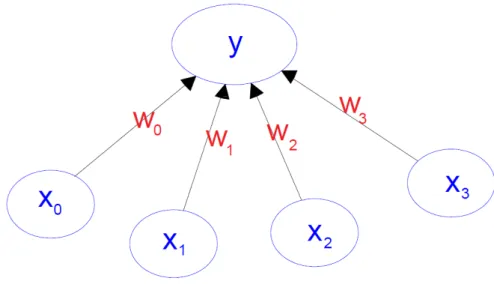
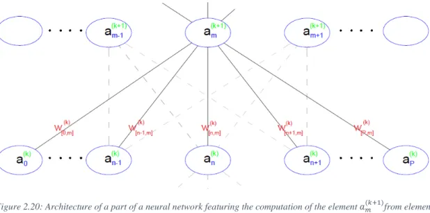
Figure 2.18: The generation of an output “y” in a simple neuron with 4 inputs ... 30

Figure 2.19: Architecture of a neural network with 1 hidden unit ... 31

Figure 2.20: Architecture of a part of a neural network featuring the computation of the element 𝑎𝑎𝑚𝑚(𝐿𝐿+ 1)from elements on layer k ... 32

Figure 2.21: Four different ways of forming clusters from a dataset (Tan, Steinback y Kumar 2006) ... 34

Figure 2.22:The dendrogram and clusters for example points p1 to p4 (Tan, Steinback y Kumar 2006) ... 35

Figure 2.23: Typical moment-curvature relation for a reinforced concrete section (Kwak Hyo 2002) ... 40

Figure 2.24: Flexion cracks that curve a little as they progress through the section of a short beam... 40

Figure 2.25: Flexion cracks in a simply supported concrete beam with a large span (Vidal 2007) ... 40

Figure 2.26: Flexion and shear crack patterns in double fixed beams (ce-ref.com s.f.) ... 41

Figure 2.27 Strut and ties model for a concrete beam (Schlaich y Shafer, Toward a consistent design of Structural Concrete 1987) ... 41

(13)

xi

Figure 2.30: Concrete beam with the bottom longitudinal reinforcement affected by corrosion

(Muñoz 1994) ... 44

Figure 2.31: Corrosion induced cracking in a beam (Du, Chan y Clark 2013) ... 44

Figure 2.32: Local bond stress-slip law (Task Group 2000) ... 45

Figure 2.33: Different viewpoint of the splitting cracks caused by the compression on the struts around reinforced bars (Task Group 2000) ... 46

Figure 2.34: Modes of bond failure: (a) pull-out failure, (b) splitting-induced pull out accompanied by crushing and shearing-off in the concrete below the ribs and (c) splitting accompanied by slip on the rib faces (Task Group 2000) ... 46

Figure 2.35:Hairlike splitting cracks along the bottom face of a beam-test specimen (Plizzari y Franchi 1996) ... 47

Figure 2.36: Crack pattern in a concreted partially prestressed beam presenting flexion, shear and bond cracks. (Duarte 2019) ... 47

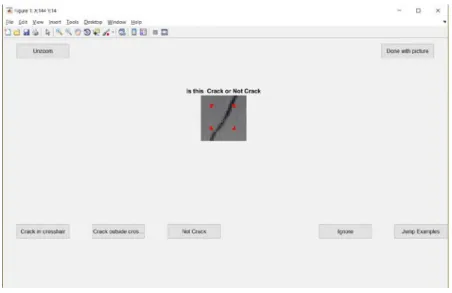
Figure 3.1: GUI panel used to classify an image patch as “Crack” or “Not Crack” to generate examples ... 51

Figure 3.2:Image patches labeled as “Crack” from the training set ... 51

Figure 3.3 Image patches labeled as “Not Crack” in the training set ... 52

Figure 3.4: Curve to determine ideal hidden layer size for the Neural Network for the Crack detection step ... 54

Figure 3.5: Architecture of the Neural Network for the Crack detection step ... 54

Figure 3.6:Learning curve for the Neural Network for the Crack detection step ... 55

Figure 3.7: Curve Error vs λ regularization term ... 56

Figure 3.8: Image patches from Test predicted as “Not Cracks” ... 57

Figure 3.9:Image patches from Test set predicted as “Crack” ... 57

Figure 3.10: Picture of a prestressed concrete beam during testing ... 58

Figure 3.11: Region of interest picked by user from picture in Figure 3-10 ... 59

Figure 3.12: Mask obtained by the NN segmentation of the picture in Figure 3-10 ... 59

Figure 3.13:Function to generate the orientation kernel ... 61

Figure 3.14: Orientation kernel for 60 degrees and a size of 25x25 pixels, viewpoint 1 ... 62

Figure 3.15: Orientation kernel for 60 degrees and a size of 25x25 pixels, viewpoint 2 ... 63

Figure 3.16: Neighborhood from an input picture and the same neighborhood segmented with the mean detection thresholding ... 63

Figure 3.17: Response of the neighborhood shown in Figure 3-16 to the orientation kernels of size m=15 ... 64

Figure 3.18: Theoretical color intensities in a line of pixels perpendicular to the crack width Where: BC is the color intensity of the background (concrete); CC is the color intensity of crack; C is the center of the line of pixels; w is the width of the crack ... 65

Figure 3.19: Color intensities in a line of pixels perpendicular to the crack width. Where: BC is the color intensity of the background (concrete); CC is the color intensity of crack ... 66

Figure 3.20: Gradient of the color intensities in a line of pixels perpendicular to the crack; Where: C is the center of the line of pixels; w is the width of the crack ... 66

Figure 3.21: Graphical resume of the transformations and processes ... 68

Figure 4.1: The projection and distances between data points 𝑃𝑃(𝑎𝑎) and 𝑃𝑃(𝑏𝑏)when the Euclidean vector 𝑉𝑉𝑉𝑉𝑉𝑉𝑐𝑐 is almost perpendicular to both crack direction vectors 𝑉𝑉(𝑎𝑎)and 𝑉𝑉(𝑏𝑏) ... 71

(14)

xii

Figure 4.3: Minimum distance “d” between a cluster “A” and a cluster “B” ... 73

Figure 4.4: Flowchart for making up the crack clusters ... 74

Figure 4.5: Artificial cracks and symbols drawn in AutoCAD to use as input for the Crack detection algorithm ... 75

Figure 4.6: Mask with the widths of the cracks after passing the image in Figure 4-5 through the Crack Detection algorithm ... 75

Figure 4.7: Mask with the angles of the cracks after passing the image in Figure 4-5 through the Crack Detection algorithm ... 76

Figure 4.8: Clusters found in the Mask presented in Figure 4-6 and Figure 4-7 ... 76

Figure 4.9: Concrete beam being tested in laboratory presenting a shear crack pattern in its web (Celada 2018)... 77

Figure 4.10: Angle Mask obtained from passing the image in Figure 4-9 through the crack detection described in chapter 3 ... 77

Figure 4.11: Result of the first step of the clustering algorithm explained in subsection 4.4.1 applied to the mask showed in Figure 4-10 ... 78

Figure 4.12: Flowchart with the steps for the cluster filtering ... 79

Figure 4.13: Clusters after merging all clusters whose endpoint crack points are close and have similar direction angles ... 79

Figure 4.14: Final clusters after removing those whose length is smaller than 30 mm ... 80

Figure 5.1: Flowchart with the inputs, model and outputs to solve the classification problem of assigning a crack pattern to a given pathology. ... 82

Figure 5.2: Crack pattern from a test beam failing in (Cladera 2003) ... 83

Figure 5.3: Photo from a test beam failing by shear (Walraven 1980) ... 83

Figure 5.4: Photo of a beam in a building with shear cracks along all its web (Muñoz 1994) .... 83

Figure 5.5: Shear Crack pattern from testing on beams with corroded shear reinforcement (Takahashi 2013) ... 83

Figure 5.6: Typical crack pattern generated by flexion and shear (Broto Xavier 2006) ... 84

Figure 5.7: A drawn crack pattern from a test in a concrete beam (Bairán, Mari y Cladera 2017) ... 84

Figure 5.8: Transformation of an example of a beam cracked by shear and flexion into a standardized image ... 84

Figure 5.9: Transformation of an example of a beam cracked by corrosion into a standardized image ... 85

Figure 5.10: Separating a standardized image example in exclusive examples (Flexion and Shear) ... 85

Figure 5.11: Transformation from the mask crack output with the angles and width into a feature matrix ... 86

Figure 5.12: Mapping of the crack pixels in the ROI inside the Angle Mask into the Feature Matrix ... 87

Figure 5.13: Mapping of the Angle mask into the depth of the Feature matrix, the depth represents the angle interval where ... 87

Figure 5.14: Transformation from the feature matrix into a feature vector ... 88

Figure 5.15: Error in Training and Test Sets vs Number of Training Examples ... 89

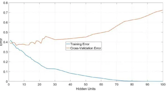
Figure 5.16: Error in Training and Test set vs Number of Hidden Units in the NN ... 90

Figure 5.17 Test and Training Error vs the regularization parameter λ ... 90

(15)

xiii

Figure 5.20: Generating a Feature matrix from each angle and width mask segmented by their

individual clusters... 93

Figure 5.21: Classification of each Feature matrix that belongs to each cluster crack with the NN designed ... 93

Figure 5.22: Final cluster classification for an example ... 94

Figure 6.1: Concrete beam I-181” loaded with 635 kN ... 95

Figure 6.2: Elevation viewpoint with the dimensions of beam I-181 ... 96

Figure 6.3: Cross-Section of beam “I-181” in the ROI focused ... 96

Figure 6.5: Region of interest (ROI) selected from the image presented in Figure 6-1 ... 96

Figure 6.6: Segmentation by means of a NN of the ROI in Figure 6-3 ... 97

Figure 6.7: Part of the Angle Mask obtained from the crack detection algorithm ... 97

Figure 6.8: Part of the Width Mask obtained from the crack detection algorithm ... 98

Figure 6.9: First part of the clustering algorithm applied on the width and angle masks from Figure 6-5 and Figure 6-6. ... 98

Figure 6.10: Second part of the clustering algorithm applied on the masks from Figure 6-5 and Figure 6-6. ... 99

Figure 6.11: Final classification mask of the example ... 99

Figure 6.12: Dimensions of the test beam “Biga 2” ... 100

Figure 6.13: Cross-section of test beam “Biga 2” ... 100

Figure 6.14: Concrete beam “Biga 2” loaded with 486 kN ... 101

Figure 6.15: Region of interest chosen from the picture presented in Figure 6-12 ... 101

Figure 6.16: Segmentation with a NN of the ROI presented in Figure 6-13 ... 102

Figure 6.17: Angle mask obtained from the crack detection algorithm ... 102

Figure 6.18: Width mask obtained from the crack detection algorithm ... 103

Figure 6.19: Clusters obtained with the first part of the clustering algorithm applied on the Width and Angle masks in Figure 6-15 and Figure 6-16 ... 103

Figure 6.20: Clusters obtained with the second part of the clustering algorithm applied on the Width and Angle masks in Figure 6-15 and Figure 6-16 ... 104

Figure 6.21: Final classification mask of the example ... 104

Figure 6.22: Beam geometry and reinforcement (Tetta, Koutas y Bournas 2015) ... 105

Figure 6.23: Cracked fiber reinforced beam (Tetta, Koutas y Bournas 2015) ... 105

Figure 6.24: ROI selected from the picture presented in Figure 6-21 ... 106

Figure 6.25: Segmentation with a NN of the ROI presented in Figure 6-22 ... 106

Figure 6.26: The Angle mask obtained for the ROI presented in Figure 6-22 ... 107

Figure 6.27: The Width mask obtained for the ROI presented in Figure 6-22 ... 107

Figure 6.28: The crack clusters obtained with the clustering algorithm from the width and angle masks presented in Figure 6-24 and Figure 6-25 ... 108

Figure 6.29: Final Classification of the Crack pattern ... 108

Figure 6.30: Concrete beam “Biga 3” loaded with 570 kN... 109

Figure 6.31: Elevation viewpoint of test beam “Biga 3” ... 109

Figure 6.32: Cross-section of “Biga 3” with its transversal and longitudinal reinforcement .... 110

Figure 6.33: Region of interest (ROI) selected from the image presented in Figure 6-28 ... 110

Figure 6.34: Mean detection segmentation of the ROI presented in Figure 6-31 ... 110

Figure 6.35: Angle mask of the photo presented in Figure 6-28 ... 111

(16)

xiv

Figure 6.38: The final classification of the crack pattern in the photo in Figure 6-28 ... 112 Figure 6.39: Photo of fiber reinforced concrete beam without transversal reinforcement after essay ... 113 Figure 6.40: Mean segmentation mask obtained from the input picture presented in Figure 6-37 ... 113 Figure 6.41: Angle mask obtained from the mean segmentation presented in Figure 6-38 .... 114 Figure 6.42: Width mask obtained from the mean segmentation presented in Figure 6-38 ... 114 Figure 6.43: Clustered crack patches obtained from the masks presented in Figure 6-39 and Figure 6-40 ... 115 Figure 6.44: Final classification of the crack pattern ... 115 Figure 6.45: Crack pattern on flange of concrete beam, the crack widths have been measured ... 116 Figure 6.46: Elevation viewpoint of test beam “I181” ... 116 Figure 6.47: Mean detection segmentation from applied on the photo presented in Figure 6-43 ... 117 Figure 6.48: Angle mask generated from the photograph presented in Figure 6-43 ... 117 Figure 6.49: Width mask generated from the photograph presented in Figure 6-43 ... 118 Figure 7.1: A general Flowchart with the steps in a complete diagnosis of concrete structures ... 123

(17)

xv

Table 2-1: The most common different dissimilarity or distance metric between data ... 35 Table 2-2: Most used linkage criteria for hierarchical clustering algorithms... 36 Table 2-3:An example with 8 data points, and each data points with 4 dimensions ... 36 Table 2-4: The cosine distances matrix between the data points presented in Error! Not a valid bookmark self-reference. ... 36 Table 3-1: Four outputs from the Neural Network for crack detection being classified with a Threshold of 0.5 ... 56 Table 3-2:Confusion matrix of the result of the NN in the Cross-Validation Set ... 58 Table 3-3: Confusion matrix of the results of the NN in the Test Set ... 58 Table 5-1: Comparison of the performance of different machine learning models for the crack pattern classification problem ... 88 Table 5-2: Confusion Matrix with the percentages of true positives, false-positives and false negatives for the predictions of the NN model in the Test set. ... 91 Table 6-1: Comparison of crack widths obtained with a measuring magnifier and ... 118

(18)

1.

Introduction

1.1.

Research relevance

Cracking of concrete elements is something expected in service conditions of reinforced (RC) and partially prestressed concrete (PPC) structures. However, it should be controlled with adequate design, in order to assure durability and serviceability. This is done to ensure the durability of the concrete structures, as wider cracks make concrete elements vulnerable to chemical attacks such as carbonation, chlorides, sulphates and alkali-silica reaction. Being able to measure with precision the width of the fissures may help improve existing models (Bazant 1979) (Ho y R 1987) to predict the advance of these attacks in existing structures as almost all of them include the crack width in the calculations.

On the other hand, existence of particular crack patterns characteristics may inadequate performance or even that a structure may be prone to failure. Many resisting models, such as the aggregate interlock (Taylor 1970) (Walraven 1980) (Zararis 1997), relate to crack width and orientation and may use them explicitly in their formulations.

Moreover, rehabilitation of structures has been a problem even before the appearance of civil engineering as a standalone field. Rehabilitation starts with the inspection, diagnosing and identification of the damage caused pathology affecting the concrete structures as most authors on works on classic rehabilitation and diagnosing have stated ((AENOR) 2009) (Elizalde Javier 1980) (Muñoz 1994) (Woodson 2009). Multiple research works have been done on rehabilitation of concrete structures featuring uses of new materials (Mikulica, Laba y Hela 2017) (Saadatmanesh 1997), improvement of known techniques (Chau-Khun, y otros 2017), new techniques (Ihekwaba, Hope y Hansson 1996). But there is certainly a lack of studies on the topic of the visual diagnosing techniques on existing structures given that this task has always been very dependent on the experience and empirical criteria rather than in mathematical models. Very recently some works on the tasks of crack detection and measurement with image processing and machine learning have made their way in the field (Gopalakrishnan y Khaitan 2017) (Davoudi, Miller y Kutz 2017) (Pauley, Peel y S. 2017) (Kim, y otros 2017) and it is the start of a new wave towards the widespread usage of these techniques.

1.2.

Motivation

Early identification of undesirable crack patterns is usually considered as an indicator of malfunctioning or the existence of pathological behavior. Identifying these patterns and analysis is essential in diagnosis and inspection. Systematic inspection of large infrastructures networks can be costly, especially in regions that are of difficult access. Moreover, recognition of patterns and their analysis requires expertise, especially experience. Therefore, automatization of this

(19)

process is relevant for cost reduction of maintenance, systematization and inspection of zones that are difficult to reach for man visual inspection. Therefore, an automatic identification and measurement system would be useful to combine with mechanical resisting models and identify need for repair a retrofit.

1.3.

Scope and objectives

1.3.1.

General objective

The general objective of this thesis is to develop a system that measures and detects cracks’ widths, lengths and able to identify the pathology that caused the given cracks. All this based on a digital color picture of a concrete surface or element.

1.3.2.

Specific objectives

The general objective can be divided and expanded with the following arguments:

•Identify and characterize cracking patterns in reinforced concrete elements from the pictures taken in bare concrete surface with a digital camera using digital image processing techniques.

•Measure the direction and width of all the cracks detected in a concrete surface.

•Develop a method to quantity the cracks in a picture and determine their separation and direction.

•Develop a method to diagnose a crack pattern on a concrete structure only from the picture of this element using Machine Learning models.

1.4.

Methodology

This Thesis uses different techniques to perform the tasks proposed in the objectives: Segmentation of the crack pixels, measuring of width and angle of cracks, Machine learning for classification and clustering of crack image patches.

The Machine Learning models for classification are validated by dividing the total training examples in Training, Cross-Validation and Test sets; training the model with the Training set and checking its performance in the unseen Cross-Validation and Tests sets.

The measurements of the crack widths and angles are validated with pictures focusing on single cracks whose widths has been measured manually with a measuring magnifier.

The results from the Segmentation of the crack pixels are evaluated subjectively by visual inspection as there is not a generally accepted way to measure in a quantitative way the performance of a segmentation algorithm.

The results from the crack clustering algorithm will be evaluated by visual inspection as they are linked to the segmentation results.

(20)

1.5.

Outline of the Thesis

This document has been divided in 7 chapters and 2 annexes being the current introduction the first of them in which the objectives, the relevance of the work and motivations are presented. In the second chapter is the description of the State of the Art, where the most important concepts, equations, criteria and methods from the different areas of knowledge involved in this document are reviewed. These range from the bases of Photogrammetry, Digital Image Processing, Diagnosis of pathologies in Concrete Structures and Machine learning. Within these sub-sections the scope are the visual diagnosing techniques for cracks, the spatial filtering, image segmentation techniques, Neural Networks (NN).

The third chapter presents the method developed to detect and measure cracks in images from concrete surfaces using Neural Networks, segmentation and spatial filtering. This method is implemented in a script from the computer program MATLAB to present its outputs. This chapter is divided in two parts: the first being a description and evaluation of the NN designed to obtain image patches which may contain cracks in the given Region of Interest (ROI). The second part of the chapter presents a proposed algorithm to detect pixels which belong to a crack and to measure the orientation and width of these cracks by means of image segmentation, spatial filtering and other digital image processing techniques.

Chapter 4 deals with a clustering a method that takes the output from the process described in chapter 3 and attempts to use a new clustering technique to group up the pixels that are labeled as cracks in clusters. This clustering method is also used to decrease the amount of false positives detection from the output of chapter 3.

In Chapter 5, the filtered output from the method described in Chapter 3 is taken as starting point to train a classifier of crack patterns for concrete beams. This classifier is used to recognize crack patterns separated with the clustering technique presented in Chapter 4 and separate cracks from different pathologies.

In Chapter 6 presents a set of case studies that allows demonstrating the capabilities of the system developed as well as validation set. Here, the methods described in chapter 3 to 5 are used on 6 images of concrete beams with cracks in their surfaces in order to show the potential and limitations of the methods proposed.

Finally, in Chapter 7 the conclusions of this work are presented together with a discussion of the potential of the methods designed and future lines of work. Recommendation for further research are also given, highlighting the possible improvements of presented methods and spark interest towards Machine Learning and Digital Image Processing for improving models, experimental techniques and methods in Civil Engineering.

Annexes A and B include the databases of the images used to train the Neural Network in chapter 3 and the Neural Network to classify crack patterns in chapter 5.

(21)

(22)

2.

State of the Art

In the following chapter, a review of the most relevant techniques of digital image analysis, Photogrammetry is presented in the context of the different application sectors in which they have been implemented. Further, the basis of machine learning is also discussed. Different applications of machine learning exist nowadays in different engineering sectors. These are analyzed with emphasis on applications to computer vision and diagnosis through images. Finally, process of inspection and assessment of a concrete structures is discussed, highlighting the phase of visual inspection and expert opinion analysis, including the previous research works carried out. The requirements of a machine learning system to this task are identified and discussed.

(23)

2.1.

Photogrammetry

The first half of this Chapter will make a brief review first on the definition of this area of knowledge, the applications in other fields, and some insight on its relation and applications on civil engineering. Then on the second half of the Chapter the theory and equations that compose the base for the photogrammetric measurements will be resumed and presented starting with the optics of thin lenses in cameras.

Definition

Photogrammetry is defined as the science of making measurements or reconstruct the object space from images. It involves a compendium of methods of image measurement and interpretation in order to measure something in one or a series of pictures. Usually, it is used to obtain coordinates of surfaces in real life units (meters, mm) and to obtain 3D reconstruction of objects. Although, Tough the spam range of applications is large and covers other fields.

2.1.2.

Types of Photogrammetry

Photogrammetry can be classified in a number of ways, but one standard approach is to divide the field based on the camera location during photography. On this basis, there are two types: “Aerial Photogrammetry”, (AP) and “Close-Range Photogrammetry” (CRP) (Walford 2010). In Aerial Photogrammetry (AP) the camera is mounted in an aircraft and is usually pointed vertically towards the ground. Multiple overlapping photos of the ground are taken as the aircraft flies along a flight path, as shown in Figure 2.1.

Figure 2.1: An airplane taking overlapping photos in an area to make a map through photogrammetric methods

In Close-range Photogrammetry (CRP) the camera is close to the subject and is typically hand-held or on a tripod. Usually the output from this process are 3D models, measurements and point clouds are used to measure buildings, engineering structures, forensic and accident scenes, mines, archaeological artifacts, film sets, etc.

2.1.3.

Applications of close-range Photogrammetry

Next, some other applications of CRP are presented: (Luhmann T 2006):

(24)

 _Engineering

 Medicine and physiology  Forensic, including police work

 _{Automotive, machine and shipbuilding industries}  _{Aerospace industry}

2.1.4.

Applications in Civil Engineering

Topography

The most widespread usage of Photogrammetry in Civil Engineering is its use in Topography, their relation goes way back to the invention of photography, as the first uses of Photogrammetry were as a tool to make-up maps, by Laussadat in 1849 (Polidori 2014), and that continues nowadays. Both fields (Topography and Photogrammetry) share the same concepts of perspective and projective geometry; and those methods are used for determining the positions of real life points.

Aerial Photogrammetry (AP) branched out from the relation Topography-Photogrammetry a while ago when the former developed its own devices (theodolites, total stations) specialized in achieving its main objective (measuring exact position of featured points in terrain in means of latitude, longitude and altitude or other local coordinate systems). Some books on aerial photogrammetry trace back to the beginning of the 20th_{century (Lüscher 1920) (Lassalle 1941)}

and the bases are still the same until the appearance of digital cameras that modified some processes to obtain the interior orientation (Luhmann T 2006) (Schenk 1999).

Generally speaking, AP is used to create topographical maps. Topographical maps are created so that both small and large geographical areas can be analyzed. In many cases, topographical maps are used in conjunction with geographic information systems (Sanders s.f.). Some other Topography-like applications works are on monitoring deformation in structures (Maas y Hampel 2006) (Albert, y otros 2002).

Digital Image Correlation

Commonly known in its short version as DIC, Digital Image Correlation is a sub-field of Photogrammetry that concerns all optical methods and formulation to obtain displacement and strain fields in 2D or 3D of objects depicted by a digital image within a region of interest (ROI) (Phillip 2012).

DIC uses image processing techniques in an attempt to solve this problem. The idea is to somehow obtain a one-to-one correspondence between object points in the reference (initial undeformed picture) and current (subsequent deformed pictures) configurations. DIC does this by taking small subsections of the reference image, called subsets, and determining their respective locations in the current configuration (block matching) (Blaber J 2015).

Algorithm Basis

There are several formulations for the task of matching a subset in an image taken in a time “𝑡𝑡” and in the next image on time “𝑡𝑡+ 1” and with this computing the displacement of that subset. The computation of the displacements starts by obtaining the correlation matrix 𝐶𝐶 between two subsets 𝑚𝑚(𝑡𝑡)_and_𝑚𝑚(𝑡𝑡+1)_{that are part of images}_𝐼𝐼(𝑡𝑡)_and_𝐼𝐼(𝑡𝑡+1)_{, one of the several expressions}

(25)

(Blaber J 2015) to obtain this is the cross-correlation equation for obtaining an element 𝑐𝑐[𝑖𝑖,𝑗𝑗] of the correlation matrix 𝐶𝐶 and presented on (2.1) :

Where [𝐿𝐿,𝑗𝑗] is the local indexing of the subset matrices 𝑚𝑚(𝑡𝑡)_,_𝑚𝑚(𝑡𝑡+1)_and_𝑚𝑚�(𝑡𝑡)_,_𝑚𝑚�(𝑡𝑡+1)_{are the} mean intensities of the subsets.

Figure 2.2: Detected displacement of subset m from time t to time t+1 (Blaber J 2015)

With the Correlation matrix, the displacement may be obtained by finding the minimum in that Correlation matrix (or maximum if (2.1) is 1− 𝑐𝑐[𝑖𝑖,𝑗𝑗]) and flagging that as the new position of subset 𝑚𝑚(𝑡𝑡)_{. In order to get a subpixel precision position, the correlation matrix can be} interpolated with an approximation to a linear, quadratic, gaussian curve or any other the user may want.

The displacement field is obtained by repeating this minimum search for all the subsets defined and interpolating it in the pixel positions that are not a subset centroid.

Strains are more difficult to resolve than the displacement fields because strains involve differentiation, which is sensitive to noise. This means any noise in the displacement field will magnify errors in the strain field. Some works involving DIC and Civil engineering have topics concerning testing of materials (Rodriguez, y otros 2012) , obtaining elastic properties (Hild y Roux 2006) (Criado, Llore y Ruiz 2013), for getting fluids particles velocity (Thielicke 2014).

2.1.5.

Mathematical Foundations

This subsection will include a resumed basis of the mathematical background behind the photogrammetric processes. Presenting a brief review on the classic physics model of thin converging lenses, an introduction on interior and exterior orientation for single camera systems

𝐜𝐜[𝐢𝐢,𝐣𝐣]= ∑ ∑ �𝐦𝐦

(𝐭𝐭)₍_𝐢𝐢_,_𝐣𝐣₎_{− 𝐦𝐦}_�(𝐭𝐭)_{��𝐦𝐦}(𝐭𝐭+𝟏𝟏)₍_𝐢𝐢_,_𝐣𝐣₎_{− 𝐦𝐦}_�(𝐭𝐭+𝟏𝟏)_�

𝐲𝐲 𝐱𝐱

(26)

including the most common optical errors (Radial Distortion and Tangential Distortion) in CRP processes.

2.1.6.

Thin Lenses

A lens with a thickness (distance along the optical axis between the two surfaces of the lens) that is negligible compared to the radius of curvature of its surface is known as a thin lens. The thin lens approximation ignores optical effects due to the thickness of lenses and simplifies ray tracing calculations. It is often combined with the paraxial approximation in techniques such as ray transfer matrix analysis. Light rays follow simple rules when passing through a thin lens, this set of assumptions is known as the paraxial ray approximation (Hecht 2002):

• Any ray that enters parallel to the axis on one side of the lens proceeds towards the focal point F on the other side.

• Any ray that arrives at the lens after passing through the focal point on the front side, comes out parallel to the axis on the other side.

• Any ray that passes through the center of the lens will not change its direction.

By tracing these rays, the relationship between the object distance ℎ and the image distance 𝑐𝑐′ is described by Eq. (2.2).

Thin lenses are one of the main components in a digital camera, as they determine how the image will be formed inside a camera. The trajectory of light rays from an object in space through thin converging lenses towards the camera sensor based on the paraxial approximation is illustrated in Figure 2.3. It is assumed that the camera uses some type of digital sensor and is not a film based camera (Luhmann T 2006).

1 ℎ+ 1 𝑓𝑓′ = 1 𝑐𝑐 (2.2)

(27)

Figure 2.3 : Ray tracing of the light going from an object in the real world through the camera lenses and into the camera sensor.

The variables presented on Figure 2.3 are: ℎ: object distance, 𝑐𝑐: principal distance, z: focal object distance, 𝑧𝑧’: focal image distance, 𝐻𝐻1 and 𝐻𝐻2: external and internal principal planes, 𝑂𝑂’:

origin of the camera coordinate system and perspective center.

2.1.7.

Interior Orientation

The first step towards reconstructing the object space from images is obtaining the interior orientation defined as the transformation between the pixel coordinate system to the camera coordinate system that are presented in the next subsection (Schenk 1999).

Pixel Coordinates

The reference system for all digital images is the pixel coordinate system. It is a coordinate system defined in 2 dimensions and measured in the pixel space, this system has the same structure as a matrix coordinate system with the rows and columns starting on the top left of the plane; this system uses only positives and integer values. This system is presented in Figure 2.6. The Fiducial center (FC) is the geometric center of the rectangle representing the digital image and is presented on Figure 2.4 together with the pixel coordinate system. 𝑃𝑃𝑟𝑟 and 𝑃𝑃𝑐𝑐 are

the height and length of a single pixel in real life length units (mm, inches).

One way to quantify the detail that the camera can capture is called the resolution (in non-Photogrammetry argot (Luhmann T 2006) ), and it is measured in pixels. The more pixels a camera has, the more detail it can capture and the larger pictures can be without becoming blurry or "grainy."

When the pixel counts are referred to as resolution, the convention is to describe the pixel resolution with the set of two positive integer numbers, where the first number is the number of pixel columns (width) and the second is the number of pixel rows (height), for example as 7680 by 6876. Another popular convention is to cite resolution as the total number of pixels in

(28)

the image, typically given as number of megapixels, which can be calculated by multiplying pixel columns by pixel rows and dividing by one million. Other conventions include describing pixels per length unit or pixels per area unit, such as pixels per inch or per square inch. None of these pixel resolutions are true resolutions, but they are widely referred to as such; they serve as upper bounds on image resolution (Kiening 2008) (Koren 1999).

Figure 2.4: Pixels coordinates of a digital image and its fiducial center (FC)

Camera Coordinates

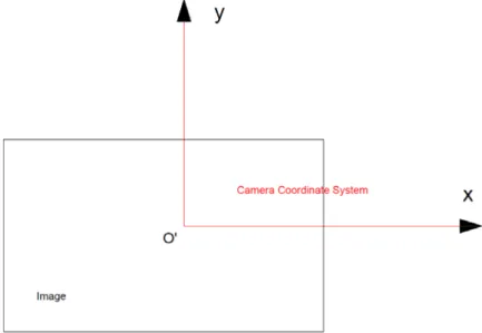
Camera coordinates are defined as the coordinates of the picture formed inside the camera by the light passing through the aperture and lenses of the camera; the origin of the camera coordinate system is placed in the Projection Center (𝑂𝑂’) and at a distance of 𝑐𝑐 (principal distance) from the plane of the sensor camera. A projection of the 2 dimensions of the parallel to the image plane is featured in Figure 2.5.

(29)

Pixel to Camera Coordinates

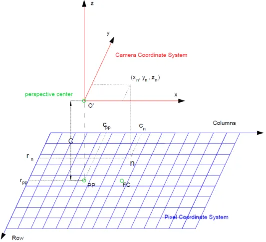
Figure 2.6 and Figure 2.7 shows in two perspectives how an arbitrary point 𝐿𝐿 in the pixel coordinate can be mapped into the camera coordinates. The point 𝐿𝐿 on the sensor can be expressed in the Pixel coordinates as [𝑟𝑟𝑛𝑛,𝑐𝑐𝑛𝑛] and then in the camera coordinates as [𝑥𝑥𝑛𝑛,𝑦𝑦𝑛𝑛,𝑧𝑧𝑛𝑛].

The projection center point projected on the sensor plane is labeled as 𝑃𝑃𝑃𝑃. 𝑃𝑃𝑟𝑟 and 𝑃𝑃𝑐𝑐 are the

dimensions of each pixel in real life units, which can be obtained by dividing the dimensions of the sensor by the number of pixels in each direction.

(30)

Figure 2.7: Perspective view to feature the projection relations between the camera coordinate system and pixel coordinate system

From the relations shown in Figure 2.7 the Eq. (2.3) can be obtained and also used to

transform a point 𝐿𝐿 in pixel coordinates [𝑟𝑟𝑛𝑛,𝑐𝑐𝑛𝑛] to camera coordinates[𝑥𝑥𝑛𝑛,𝑦𝑦𝑛𝑛,𝑧𝑧𝑛𝑛]: �𝑥𝑥𝑦𝑦𝑛𝑛𝑛𝑛 𝑧𝑧𝑛𝑛 �=��𝑐𝑐₋𝑛𝑛₍_𝑟𝑟− 𝑐𝑐_𝑛𝑛_{− 𝑟𝑟}𝑝𝑝𝑝𝑝_{𝑝𝑝𝑝𝑝}�+₎_𝑃𝑃𝑃𝑃_𝑟𝑟𝑐𝑐 −𝑐𝑐 � (2.3) Correction functions

The camera coordinates are subject to deviations from the ideal central perspective model. These are derived from the imperfections of the optical elements of cameras. In order to compensate such deviations, a correction function is defined. The expression for the corrected coordinates takes the form described in (2.4) (Luhmann T 2006).

�𝑦𝑦′𝑥𝑥′𝑐𝑐𝑐𝑐𝑟𝑟𝑐𝑐𝑐𝑐𝑟𝑟 𝑧𝑧′𝑐𝑐𝑐𝑐𝑟𝑟 �=�𝑥𝑥 ′₊_𝑥𝑥 𝑝𝑝+∆x′ 𝑦𝑦′₊_𝑦𝑦 𝑝𝑝+∆𝑦𝑦′ −𝑐𝑐 � (2.4)

The distance 𝑐𝑐 was presented before on Figure 2.3 and Figure 2.7 . The origin of the camera coordinates lies on the projection center(PP) and it usually does not coincide with the perfect center of the plane rectangle where the picture lies (Fiducial Center, FC). The offset from the center of the rectangle in camera coordinates is labeled as (𝑥𝑥𝑝𝑝,𝑦𝑦𝑝𝑝) and is obtained through the

camera calibration to measure the radial and tangential distortion which will be presented below.

(31)

Radial Distortion

Radial distortion constitutes the main source of imaging error for most camera systems. It is attributable to variations in refraction at each individual component lens within the objective. It is a function of the lens design, chosen focal length, object distance. Visually, it looks as going from a perfectly aligned grid with parallel grid lines, to a barrel-like distortion or pincushion deformation, as illustrated in Figure 2.8.

Figure 2.8: Deformation of coordinates caused by barrel and pincushion type of distortion (Luhmann T 2006)

One of the better-known models for radial distortion is the one developed with polynomial series by Brown in 1971 (Brown 1966). In Brown’s model, the radial distortion takes the form of Eq. (2.5).

∆𝑟𝑟′

𝑟𝑟𝑟𝑟𝑟𝑟=𝐾𝐾1𝑟𝑟+𝐾𝐾2𝑟𝑟3+𝐾𝐾3𝑟𝑟5+𝐾𝐾4𝑟𝑟7… (2.5)

Where 𝑟𝑟 is the radial distance of each point with respect to the origin of the camera coordinates system, computed as in (2.6). In this equation, 𝑥𝑥′_,_𝑦𝑦′_,_𝑦𝑦

𝑝𝑝,𝑥𝑥𝑝𝑝 are in camera coordinates. Then,

the radial distortion correction terms, for 𝑥𝑥 and 𝑦𝑦 directions, are computed as in Eq. (2.7). 𝑟𝑟2₌_{�𝑥𝑥′ − 𝑥𝑥} 𝑝𝑝�2+�𝑦𝑦′ − 𝑦𝑦𝑝𝑝�2 (2.6) ∆𝑥𝑥′𝑟𝑟𝑟𝑟𝑟𝑟=𝑥𝑥′∆𝑟𝑟 ′_{𝑟𝑟𝑟𝑟𝑟𝑟} 𝑟𝑟′ ∆𝑦𝑦′𝑟𝑟𝑟𝑟𝑟𝑟=𝑦𝑦′ ∆𝑟𝑟′_{𝑟𝑟𝑟𝑟𝑟𝑟} 𝑟𝑟′ (2.7) Tangential Distortion

Another source of deviation is the tangential distortion, also called Radial-asymmetric distortion. This error is caused by decentering and misalignment of individual lens elements within the objective, as shown in Figure 2.9. This error can be measured with Eq. (2.8), proposed by Brown (Brown 1966).

∆𝑥𝑥′

(32)

The order of magnitude of the tangential distortion is typically smaller than radial distortion; hence, this correction is only used if high accuracy is needed.

Figure 2.9: Visual representation of the misalignment between the camera sensor and the lenses causing tangential distortion (Mathworks, Camera Calibration 2016)

The total correction for the camera coordinates due to distortion would have the form: ∆𝑥𝑥′ ₌_{∆𝑥𝑥′}

𝑟𝑟𝑟𝑟𝑟𝑟+∆𝑥𝑥′𝑡𝑡𝑟𝑟𝑛𝑛 ∆𝑦𝑦′ =∆𝑦𝑦′𝑟𝑟𝑟𝑟𝑟𝑟+∆𝑦𝑦′𝑡𝑡𝑟𝑟𝑛𝑛 (2.9)

2.1.8.

External Orientation

This subsection will review the bases for obtaining the exterior orientation parameters for single camera systems. The exterior orientation can be defined as the set of steps to transform points in the camera coordinates to the real-life coordinates or object coordinate system.

Image Scale

The distances used for obtaining the image scale (relation between distances in object coordinates and distances in camera coordinates) are shown in Figure 2.10.

(33)

Figure 2.10 :Relation between object distance, principal distance and the camera and real coordinates (Luhmann T 2006)

The image scale value (𝑚𝑚 or 𝑀𝑀) can be obtained with the relation between measurement of a distance 𝑋𝑋 on the object space and its equivalent in the camera space𝑥𝑥’ another way would be from the ratio of object distance ℎ to the principal distance 𝑐𝑐 and. The equation describing this relation is (2.10): 𝑚𝑚=ℎ 𝑐𝑐= 𝑋𝑋 𝑥𝑥′= 1 𝑀𝑀 (2.10)

Camera to Object Coordinate system

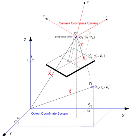
The object coordinate system is the one defined around the real-life objects depicted in the images. The transformation from the camera coordinates to the object coordinate system will depend in the type of camera used, the number of cameras and the number of points with known coordinates. All of them based on the projective geometry shown in Figure 2.11 and thin lens model presented before in Figure 2.3. The transformation from a point 𝐿𝐿’ in the camera coordinates to point 𝐿𝐿 in the object coordinate system is described in Figure 2.11 and Eq. (2.11) and (2.12) (Luhmann T 2006).

(34)

Figure 2.11: Projection relations between the camera coordinate system and the object coordinate system

𝑋𝑋⃗ is the 3 components vector that defines the position in space of a generic point 𝐿𝐿in the object coordinate system. 𝑋𝑋⃗0 is a 3 components vector that defines the position in space of the

perspective center (O’). Finally, 𝑥𝑥′��⃗ is the 3 components vector that defines the point 𝐿𝐿’ in camera coordinates

On the other hand, 𝜑𝜑,𝜔𝜔,𝜀𝜀 are the rotation angles between the object coordinate system axes X, Y, Z and the camera coordinate system axes 𝑥𝑥’,𝑦𝑦’,𝑧𝑧’. From these quantities, the rotation matrix can be obtained, Eq. (2.11):

𝑅𝑅=�𝑐𝑐𝑐𝑐𝑀𝑀𝜔𝜔𝑀𝑀𝐿𝐿𝐿𝐿𝜀𝜀𝑐𝑐𝑐𝑐𝑀𝑀𝜑𝜑+𝑀𝑀𝐿𝐿𝐿𝐿𝜔𝜔𝑐𝑐𝑐𝑐𝑀𝑀𝜀𝜀𝑀𝑀𝐿𝐿𝐿𝐿𝜑𝜑𝑐𝑐𝑐𝑐𝑀𝑀𝜀𝜀 𝑐𝑐𝑐𝑐𝑀𝑀𝜔𝜔𝑐𝑐𝑐𝑐𝑀𝑀𝜀𝜀 − 𝑀𝑀𝐿𝐿𝐿𝐿𝜔𝜔𝑐𝑐𝑐𝑐𝑀𝑀𝜑𝜑𝑐𝑐𝑐𝑐𝑀𝑀𝜀𝜀𝑀𝑀𝐿𝐿𝐿𝐿𝜑𝜑𝑀𝑀𝐿𝐿𝐿𝐿𝜀𝜀 𝑀𝑀𝐿𝐿𝐿𝐿𝜔𝜔𝑀𝑀𝑉𝑉𝐿𝐿𝜑𝜑𝑐𝑐𝑐𝑐𝑀𝑀𝜑𝜑

𝑀𝑀𝐿𝐿𝐿𝐿𝜔𝜔𝑀𝑀𝐿𝐿𝐿𝐿𝜀𝜀 − 𝑐𝑐𝑐𝑐𝑀𝑀𝜔𝜔𝑀𝑀𝐿𝐿𝐿𝐿𝜑𝜑𝑐𝑐𝑐𝑐𝑀𝑀𝜀𝜀 𝑀𝑀𝐿𝐿𝐿𝐿𝜔𝜔𝑐𝑐𝑐𝑐𝑀𝑀𝜀𝜀 +𝑐𝑐𝑐𝑐𝑀𝑀𝜔𝜔𝑀𝑀𝐿𝐿𝐿𝐿𝜑𝜑𝑀𝑀𝐿𝐿𝐿𝐿𝜀𝜀 𝑐𝑐𝑐𝑐𝑀𝑀𝜔𝜔𝑐𝑐𝑐𝑐𝑀𝑀𝜑𝜑� (2.11)

Then the transformation from an image point in camera coordinates to object coordinates is set by the collinearity Eq. (2.12), based from the relations shown in Figure 2.11.

(35)

2.2.

Digital Image Processing

Image processing and Photogrammetry has been increasingly used the last decades as the applications spread to all science. Researchers and engineers realize these techniques enable measurements and detection with low cost and with little or no affectation to the system performance.

A digital image may be defined as a two-dimensional function, 𝐼𝐼(𝑥𝑥,𝑦𝑦), where x and y are spatial coordinates, and the amplitude of 𝐼𝐼 at any pair of coordinates (𝑥𝑥,𝑦𝑦) is called the intensity or gray level of the image at that point. When 𝑥𝑥, 𝑦𝑦 and the amplitude of 𝐼𝐼 are all finite, discrete quantities, the image can be called a digital image. The field of digital image processing refers to managing information in digital images by means of a digital computer.

There are no clear boundaries in the continuum from image processing at one end to the field of computer vision at the other. However, attempts of categorizing the processes can be done as follows:

Low-level imaging processes

These processes involve primitive operation such as: Intensity Transformations, Spatial Filtering, Frequency Domain Filtering, Logarithmic and Contrast-Stretching Transformations; Histogram transformations.

Mid-level processes

These processes involve tasks such as: segmentation (partitioning an image into regions or objects), Edge detection, Corner detection, Image Sharpening, Hough Transform, Morphological operations,

High-level processes

High-level processes involve “making sense” of an ensemble of recognized objects, as in image analysis, and at the far end of the continuum, performing the cognitive functions normally associated with human vision such as: neural networks for object recognition, convolutional neural networks, pattern matching, etc. (Gonzalez, Woods y Eddins 2010).

In the following subsections, a brief review will be made on the topics within digital image processing that are used with this work.

2.2.1.

Spatial Filtering

Spatial filtering or neighborhood processing is an image operation where each pixel value 𝑓𝑓(𝑥𝑥,𝑦𝑦) is changed by a function of the intensities of pixels in a neighborhood around pixel (𝑥𝑥,𝑦𝑦). It consists of mainly 4 steps (Gonzalez, Woods y Eddins 2010):

• Selecting a center point (𝑥𝑥,𝑦𝑦) in the image

• Performing a number operation that involves only the pixels in a predefined neighborhood about (𝑥𝑥,𝑦𝑦).

• Letting the result of that operation be the response of the process at that point, it may replace previous point or fabricate a new matrix with only the response values

• Repeating the process for all the pixels in the image.

If the operations performed on the pixels of the neighborhoods are linear, the operation is called linear spatial filtering; otherwise, the filtering is referred as non-linear.

Most of the operations performed in spatial filtering fall in the category of linear spatial filtering. Most linear operation usually used imply the multiplication of each element in the neighborhood

(36)

matrix 𝑼𝑼(𝑥𝑥,𝑦𝑦) sized 𝑁𝑁 x 𝑁𝑁 pixels by another matrix 𝐻𝐻 with the same size and then sum all the elements from the resulting matrix to obtain the response 𝑅𝑅(𝑥𝑥,𝑦𝑦)) in the given point, this operation is called “correlation”, when one the operators (𝑈𝑈,𝐻𝐻) is flipped in both directions the operation is called “convolution”.

In the previous type of operations, the matrix H is commonly known as “filter”, “filter mask”, “mask”,” kernel”, template” and its elements will have special characteristics depending on the transformation that is wanted for the input picture. In many implementations, the fastest way to do correlation between a kernel and 2D matrix is by using the Convolution theorem (Arfken 1985) which transforms the regular correlation or convolution operation into a pointwise multiplication between the Fourier Transform of each argument and the result should be transformed back with the Inverse Fourier Transform. The convolution between functions 𝑓𝑓 and 𝑔𝑔 is shown in Eq. (2.14).

𝑓𝑓 ∗ 𝑔𝑔=𝐹𝐹−1_�𝐹𝐹_{_𝑓𝑓_{} .} _𝐹𝐹_{_𝑔𝑔_}_� _(2.13)

For images in the 2D discrete space, the convolution between an image function 𝑓𝑓(𝑥𝑥,𝑦𝑦) and a kernel 𝐻𝐻(𝑥𝑥,𝑦𝑦) can be defined as:

𝑅𝑅(𝑥𝑥,𝑦𝑦) =𝑓𝑓(𝑥𝑥,𝑦𝑦) ∗ 𝐻𝐻(𝑥𝑥,𝑦𝑦) = � � 𝑓𝑓(𝐿𝐿,𝑗𝑗) .𝐻𝐻(𝑥𝑥 − 𝐿𝐿,𝑦𝑦 − 𝑗𝑗) ∞ 𝑖𝑖=−∞ ∞ 𝑗𝑗=−∞ (2.14)

Following the strict mathematical definition this operation is defined in an infinite 2D space (Arfken 1985); so, in the discrete space needs to be limited to the size of the input image. An example of the output function from the convolution between a small 3x3 pixels input matrix and a 3x3 kernel matrix is presented in Figure 2.12. The way to compute every element 𝑅𝑅(𝑥𝑥,𝑦𝑦)

is done by flipping the kernel matrix in the horizontal and vertical direction and sliding it through the input 𝑓𝑓, then if the kernel is centered (aligned) exactly at the element 𝑅𝑅(𝑥𝑥,𝑦𝑦) being computed, the next step is to multiply the kernel cells by the overlapped input cells. It should be noted that the resulting matrix 𝑅𝑅 domain is usually limited to have same size as the input matrix.

Figure 2.12: Example of the resulting matrix between a convolution operation done between an input matrix and a Sobel kernel (Sobel 1968)

For further explanation, the Figure 2.13 shows the computation of the element 𝑅𝑅(1,1) in the upper left corner of the output convolution matrix:

(37)

Figure 2.13: Computation of element R(1,1) of the output matrix

Then the result would be obtained with the following summations:

𝑅𝑅(1,1) = 0∗1 + 0∗2 + 0∗1 + 1∗0 + 2∗0 + 0∗(−1) + 4∗(−2) + 5∗(−1) =−13

2.2.2.

Feature detection

Feature detection is the process of finding any aspect of interest, referred as features, that exists in digital photographs. There is no universal or exact definition of what constitutes a feature, and the exact definition often depends on the problem or the type of application. A feature can be defined as an "interesting" part of an image, and features are used as a starting point for many computer vision algorithms. Since features are used as the starting point and main primitives for subsequent algorithms, the overall algorithm will often only be as good as its feature detector. Consequently,