Open Access Dissertations Theses and Dissertations
8-2016
The design and statistical analysis of single-cell
RNA-sequencing experiments
Faye H. Zheng
Purdue UniversityFollow this and additional works at:https://docs.lib.purdue.edu/open_access_dissertations Part of theStatistics and Probability Commons
This document has been made available through Purdue e-Pubs, a service of the Purdue University Libraries. Please contact [email protected] for additional information.
Recommended Citation
Zheng, Faye H., "The design and statistical analysis of single-cell RNA-sequencing experiments" (2016).Open Access Dissertations. 897.
PURDUE UNIVERSITY GRADUATE SCHOOL Thesis/Dissertation Acceptance
This is to certify that the thesis/dissertation prepared By Faye H. Zheng
Entitled
The Design and Statistical Analysis of Single-Cell RNA-Sequencing Experiments
For the degree of Ph.D.
Is approved by the final examining committee:
To the best of my knowledge and as understood by the student in the Thesis/Dissertation Agreement, Publication Delay, and Certification Disclaimer (Graduate School Form 32), this thesis/dissertation adheres to the provisions of Purdue University’s “Policy of Integrity in Research” and the use of copyright material.
Approved by Major Professor(s): Rebecca W. Doerge
Approved by: Hao Zhang 7/7/2016
SINGLE-CELL RNA-SEQUENCING EXPERIMENTS
A Dissertation Submitted to the Faculty
of
Purdue University by
Faye H. Zheng
In Partial Fulfillment of the Requirements for the Degree
of
Doctor of Philosophy
August 2016 Purdue University West Lafayette, Indiana
ACKNOWLEDGMENTS
On the academic front, I can only begin by thanking my advisor, Rebecca W. Doerge, for being a guiding presence right from the beginning, when I entered as a doe-eyed first-year with everything to learn. Throughout the graduate school pro-cess, Rebecca has been an essential source of advice, trust, and friendship. I am also grateful to my committee members - Bruce Craig, Hyonho Chunh, Gayla Olbricht, and Tim Ratliff - for their helpful suggestions which provided direction for this work. The data which Dr. Ratliff graciously allowed me to use played an integral role in my research. I would also like to recognize professor James Eberwine and the dozen students I met at the 2014 Single Cell Analysis course at Cold Spring Harbor Labo-ratory. These were a formative few weeks in my understanding and engagement with the field; I could hardly believe how fun it was to wield a pipette and talk endlessly about biology.
I have benefited greatly from interactions among the RWD research group. Those who graduated before me - Jeremiah Rounds, Sanvesh Srivastava, Chee Chen, Doug Baumann, Tilman Achberger - set high standards in how to ask good questions, give spotless talks, and engage in academic citizenship. Present members - Patrick Medina, Emery Goossens, Ji Hwan Oh, Nadia Atallah, Yumin Zhang - always bring something interesting to the discussion table, and must be commended for sitting through endless practice talks. The graduate school experience would be nothing without good company. April, Kelly-Ann, Xiaosu, Kylie - my friends and my cohort, with whom I shared the long road of classes to quals to research. Nithin, Ana, Jeff, and Shaili my fellow running, climbing, and 14er enthusiasts. Ruth and Brittany -fellow Women in Science Program members who met my worries with empathy and shared my successes with glee.
To my parents, who have always given me full independence to occupy my life with my own choices, even the offbeat ones all taken in stride. I have been greatly affected by your boundless confidence, no matter where I go or what I do. To my brother Shawn, whom I’ve had the distinct pleasure of watching develop into an exceptionally mature and hardworking young man. That we share the same genes I consider a wonder and something of a bragging right. To my chosen sisters - Robin, Anqi, and Rochelle - for our longstanding friendships that keep getting richer despite great distances. And finally to Benjamin, for bringing to my life such humor, steadiness, and perspective - I appreciate you every day.
TABLE OF CONTENTS
Page
LIST OF TABLES . . . vii
LIST OF FIGURES . . . viii
ABBREVIATIONS . . . xi
ABSTRACT . . . xii
1 Introduction . . . 1
1.1 History of Sequencing Technologies . . . 2
1.2 Next-Generation Sequencing: From Tissues to Cells . . . 2
1.3 RNA-Sequencing . . . 4
1.3.1 Basics of RNA . . . 4
1.3.2 The Process of RNA-Seq . . . 6
1.3.3 Bulk Tissue vs. Single Cell Protocols . . . 9
2 Experimental Design of scRNA-Seq Experiments . . . 11
2.1 Sequencing Depth and Replication . . . 11
2.2 Procedure for Simulating scRNA-seq Data . . . 15
2.3 Simulations . . . 18
2.4 Guiding the Choice of Optimal Experimental Design . . . 22
2.4.1 Statistical Power Calculation . . . 25
2.4.2 Cost Function . . . 32
2.4.3 Pilot Data . . . 34
3 Modeling Differential Gene Expression from scRNA-Seq Data . . . 41
3.1 The Stochastic Nature of Gene Expression . . . 42
3.2 Existing Methods for Bulk RNA-Seq Data . . . 45
3.3 Accounting for Bimodality . . . 47
3.4 Accounting for Unmeasured Cell Cycle Effects . . . 51
3.4.1 Methods Employing Control Genes . . . 52
3.4.2 Surrogate Variable Analysis . . . 54
3.5 Simulations . . . 56
3.5.1 Simulation Results . . . 57
3.6 Experimental Data . . . 62
3.6.1 Dataset Descriptions . . . 62
3.6.2 Data Analysis . . . 63
3.6.3 Sasagawa et al. (2013) Results. . . 64
Page
3.7 Discussion . . . 69
4 Summary . . . 71
4.1 Summary of Work . . . 71
4.1.1 Design of scRNA-Seq Experiments . . . 71
4.1.2 Modeling Differential Gene Expression from scRNA-Seq Data 73 4.2 Future Work . . . 74
LIST OF REFERENCES . . . 77
LIST OF TABLES
Table Page
1.1 RNA-seq data are typically represented as a matrix of the following form.
The values yig represent the expression of gene g in samplei. The library
sizes, Li =
G
g=1yig, are the total number of reads aligned to sample i
across all genes. . . 9
2.1 Simulated datasets are generated from the real prostate dataset, by
ran-domly selecting N replicates per experimental group in the real data, and
resampling counts to the desired depth D. 50 datasets are simulated for
each combination of D×N, and edgeR is applied to obtain lists of
differ-entially expressed genes detected in each setting. . . 19
2.2 Table of outcomes when testing G simultaneous hypotheses, π0 of which
are true nulls. . . 27
2.3 Some typical costs associated with various stages of the scRNA-seq
work-flow, from cell capture to sequencing; these numbers are based on the
LIST OF FIGURES
Figure Page
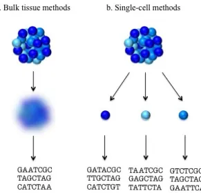
1.1 Bulk tissue sample (left) is used to obtain sequence information on an
aggregate of the entire population of thousands to millions of cells within a tissue. A single-sampled cell (right) allows for genetic heterogeneity to be dissected by obtaining sequence information on each cell within the
population of cells. . . 3
1.2 The Central Dogma of Biology [Crick et al., 1970] depicts the flow of
genetic information. DNA is the genetic code; RNA (specifically, mRNA) are transcribed copies of genes located on the DNA; these mRNA are
translated into proteins that carry out function. . . 5
1.3 NGS workflow featuring the Illumina sequencing by synthesis (SBS)
tech-nology [Illumina, Inc., 2015b]. A.cDNA is randomly fragmented into
mil-lions of pieces and adaptors are ligated to the ends. B.The fragments are
attached to the surface of the sequencing flow cell, then copied thousands of times, creating distinct clusters containing identical copies of the same
fragment. C. SBS proceeds by washing fluorescently labeled nucleotides
onto the flow cell, and using digital imaging to identify the bases as they are incorporated; this cycle is repeated one-by-one for each consecutive
base until the desired lenth of sequenced reads is achieved. D. Reads are
aligned to a reference genome using computational tools. . . 8
2.1 In the context of RNA-seq, sequencing depth most commonly refers to the
total number of reads that are mapped to the genome and subsequently
quantified as gene expression measurements. . . 12
2.2 Saturation curves of randomly chosen samples from a real scRNA-seq data
set on human prostate cancer cell lines. Each curve plots the number of detected genes, defined as genes with counts greater than 3, against against sequencing depth for a cell sample. For a full description of how this plot was generated, see Tarazona et al. [2011]. As the number of reads increase, the number of genes detected also increases, but begins to taper off. This
pattern is typical of both bulk and single-cell RNA-seq data. . . 13
2.3 Count data from a real scRNA-seq experiment (left) provide the
param-eters that are used to generate simulated gene counts (right). Mean-variance plots of the simulated gene expression data suitably mimic that
Figure Page
2.4 Results from datasets subsampled from the real prostate data, to
vary-ing sequencvary-ing depths and replicates per group. Plots depicted show the statistical power to detect DE genes (top) and the number of differen-tially expressed (DE) genes detected (bottom). Lines represent
replica-tion levels and x-axis depicts sequencing depths. The width of the gray
line corresponds to the 95% confidence interval of the mean over multiple
simulations. . . 20
2.5 Results from datasets subsampled from the real prostate data, to
vary-ing sequencvary-ing depths and replicates per group. A separate ROC curve is depicted for each of the considered replication levels per group, and
individual lines represent sequencing depths. . . 21
2.6 Statistical power to detect DE genes (top) and number of differentially
expressed (DE) genes detected (bottom), for varying combinations of se-quencing depths (in millions of reads) and replicates per group. The width of the gray line corresponds to the 95% confidence interval of the mean number of DE genes over simulation replicates at each setting. Plots were generated from synthetic data simulated using distributional parameters
extracted from the human prostate scRNA-seq dataset. . . 23
2.7 ROC curves for each of the considered replicate numbers per group. Lines
in each curve represent the sequencing depth. Plots were generated from simulated data generated using distributional parameters extracted from
the human prostate scRNA-seq dataset. . . 24
2.8 At a given depth of two million reads, the theoretical and empirical
es-timates of statistical power are similar, with empirical calculations being
slightly more conservative. . . 32
2.9 Extrapolations made from pilot prostate data of various sizes exhibit
variance-mean plots that look reasonably similar to the original full dataset
of 200 replicates and depth of 2 million (lower right). . . 36
2.10 ROC plots, one for each replication level with lines representing sequencing depth, show how accurately extrapolations from pilot datasets of each size
recover the true DE genes simulated in the full dataset. . . 37
2.11 Concordance plots depict the fraction of matching genes in a list of top
k ranking genes, identified in the extrapolated datasets as compared to
the full dataset. Each plot shows results for one depth setting, with lines
Figure Page
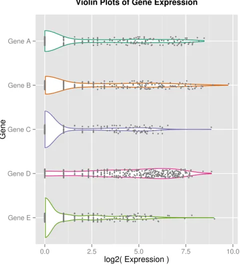
3.1 Violin plots of log counts for five randomly selected genes across 399 human
prostate cells demonstrate the bimodality, or ‘dropout events’, commonly seen in scRNA-seq data. This bimodality may arise from both biological as well as technical sources. Each point represents a cell’s expression value for a given gene, with a vertical jitter added for visual clarity. The lines display a smoothed kernel density for visualizing the overall distribution
of expression values. . . 44
3.2 The cell cycle is a series of steps that define the life span of the cell, and
are divided into the following phases: the first and longest growth phase (G1) when cells grow larger and increase their production of proteins and ribosomes in preparation for DNA synthesis; the synthesis phase (S) when cells replicate a complete copy of their DNA; the second growth phase (G2) when cells continue to prepare metabolically for mitosis; and finally,
mitosis (M) during which active cell division occurs. . . 45
3.3 SVA estimates of cell cycle across correlation settings, for selected
replica-tion levels of 25 and 200 replicates per group. Each point represents the
SVA estimate of a cell, and is colored by the true cell cycle. . . 58
3.4 ROC curves that compare ZINB and edgeR, both with and without SVA
adjustment, for each combination of replicates per group and level of
cor-relation between the group and cell cycle variable. . . 60
3.5 Concordance plots depicting the similarity in gene rankings between each
method (ZINB and edgeR, both and without SVA adjustment), for each
combination of replicates per group and level of correlation between the
group and cell cycle variable. . . 61
3.6 SVA estimates for each cell in the Sasagawa et al. (2013) data, colored by
true cell cycle. See Figure 3.2 for cell cycle descriptions. . . 65
3.7 Sasagawa et al.(2013) results. ROC plot for detecting differential
expres-sion between experimental conditions. . . 66
3.8 Sasagawa et al. (2013) results. Concordance plot depicting the similarity
in gene rankings between each method and the true gene ranks. . . 66
3.9 SVA estimates for each cell in the Buettner et al. (2015) data, colored by
true cell cycle. . . 67
3.10 Buettner et al. (2015) results. ROC plot for detecting differential
expres-sion between experimental conditions. . . 68
3.11 Buettner et al. (2015) results. Concordance plot depicting the similarity
ABBREVIATIONS
BFGS Broyden-Fletcher-Goldfarb-Shanno (algorithm)
BH Benjamini-Hochberg
cDNA complementary DNA
CML conditional maximum likelihood
DE differential expression, differentially expressed
DNA deoxyribonucleic acid
FACS fluorescence-activated cell sorting
FDR false discovery rate
FPR false positive rate
GLM generalized linear model
mESC mouse embryonic stem cell
mRNA messenger RNA
NB negative binomial
NGS next-generation sequencing
PCA principal component analysis
PrE primitive endoderm (cell)
RNA ribonucleic acid
RNA-seq RNA-sequencing
ROC receiver operating characteristic (curve)
SBS sequencing by synthesis
scRNA-seq single-cell RNA-seq
SVA surrogate variable analysis
UMI unique molecular identifiers
TPR true positive rate
ABSTRACT
Zheng, Faye H. Ph.D., Purdue University, August 2016. The Design and
Statisti-cal Analysis of Single-Cell RNA-Sequencing Experiments. Major Professor: R.W.
Doerge.
Next-generation DNA- and RNA-sequencing (RNA-seq) technologies have ex-panded rapidly in both throughput and accuracy within the last decade. The mo-mentum continues as emerging techniques become increasingly capable of profiling molecular content at the level of individual cells. One goal of this research is to put forward best practices in the design of single-cell RNA-sequencing (scRNA-seq) exper-iments, specifically as it relates to choices regarding the trade-off between sequencing depth and sample size. In addition to general guidelines, an interactive tool is pre-sented to aid researchers in making experiment-specific decisions that are informed by real data and practical constraints. Further, a new approach to the modeling and testing of differential gene expression in scRNA-seq data is proposed, which notably
incorporates salient features (e.g. highly zero-inflated expression values) of single-cell
transcription that are otherwise obscured at the tissue level. As single-cell technolo-gies offer an unprecedented window into cell-to-cell heterogeneity and its biological consequences, it is essential that suitable approaches are adopted for both the design and analysis of these experiments.
1. INTRODUCTION
Next-generation DNA- and RNA-sequencing technologies have expanded rapidly in both throughput and accuracy within the last decade. The momentum continues as emerging techniques become increasingly capable of profiling molecular content at the level of individual cells. Cell-to-cell heterogeneity and its biological consequences are now the focus of many unprecedented studies capable of illuminating the dynamic nature of single cells. Recent investigations have pushed the boundaries of under-standing structural changes in cancer genomes, varying paths of cell differentiation, and finer mechanisms of cell regulation. Like many emerging technologies, the sta-tistical analysis of single-cell data currently remains in the exploratory stage, but is poised to shift towards informative tests of specific hypotheses. Moving forward, thoughtful decisions regarding experimental design are essential if these experiments are to be maximally efficient, reproducible, and informative. One of the overarching goals of this research is to put forward best practices in the design of single-cell RNA-sequencing (scRNA-seq) experiments, specifically as it relates to choices regarding the trade-off between sequencing depth and sample size.
Aside from experimental design, the statistical analysis of scRNA-seq data itself invites a critical revisitation of standard RNA-seq methods. In particular, the model-ing and testmodel-ing of differential gene expression is currently addressed by implementmodel-ing a variety of standard and available methods which incorporate salient features of tissue-level RNA-seq data. Because these current methods do not adequately extend to RNA-seq data from single cells, another goal of this work is the development of a novel approach for the detection of differential gene expression signatures between subpopulations of single cells; this is essential, given the great interest in understand-ing cell-to-cell heterogeneity.
1.1 History of Sequencing Technologies
The aim of DNA sequencing technologies is to decipher the order of nucleotides
(i.e., the adenine, thymine, cytosine, and guanine units, collectively called bases) in a
DNA molecule, which constitutes the genetic code of an organism. Sanger sequencing marked the inception of these technologies, and culminated in the completion of the landmark Human Genome Project in 2001 [Lander et al., 2001]; this feat ushered in the age of genomics. The second wave of sequencing methods, beginning in 2004 and widely used today, brought with it substantial increases in speed and throughput. The parallel, automated nature of the process, commonly dubbed “next-generation sequencing” (NGS), produces millions of sequences concurrently, increasing through-put by many orders of magnitude [Metzker, 2010]. In addition, these high-throughthrough-put sequencing technologies have significantly decreased the cost of sequencing, which is now less than ten cents per megabase [National Human Genome Research Institute, 2015].
1.2 Next-Generation Sequencing: From Tissues to Cells
NGS procedures have become more affordable, ubiquitous, even routine, and yet the ceiling of optimization is being pushed still further. Capitalizing on well-established NGS platforms, recent technological advances have enabled a dramatic scaling down in the amount of genomic starting material required to produce se-quence information. Indeed, it is now possible to sese-quence at the level of individual cells. In the past, genomic data generated by NGS procedures typically came from aggregating the entire population of thousands to millions of cells within a tissue (Figure 1.1), even though it is increasingly understood that genetic heterogeneity is the norm rather than the exception [Eberwine et al., 2014]. The bulk pooling of cell populations averages out differences between the behaviors of individual cells, blends together the patchwork composition of cells within certain tissues, and obscures the dynamic nature of cellular function. Sequencing at the single cell level allows for
the dissection of genetic heterogeneity with the intent of obtaining a much higher resolution of information.
Figure 1.1. Bulk tissue sample (left) is used to obtain sequence informa-tion on an aggregate of the entire populainforma-tion of thousands to millions of cells within a tissue. A single-sampled cell (right) allows for genetic het-erogeneity to be dissected by obtaining sequence information on each cell within the population of cells.
The ability to ask questions of individual cells has motivated a flood of research in pursuit of insights into both new and longstanding questions that previously could not be answered from bulk tissue analysis [Shapiro et al., 2013]. Living tissues are often comprised of a multitude of cell types with different lineages, stages of development, and function within the tissue. Cell lineage is particularly important in the study of in-tratumor heterogeneity; several single-cell sequencing studies have shown that tumor development occurs through a series of somatic mutations that drive groups of cells into distinct clonal subpopulations, each with its own mutational signatures and even drug response [Navin et al., 2011, Alexandrov and Stratton, 2014, Yates and Camp-bell, 2012]. Single-cell technologies have also made it possible to detect the presence
of cancer by way of rare circulating tumor cells in blood specimens [Ramsk¨old et al.,
sequencing allows for the isolation and characterization of complex microbes in the environment, offering a way to detect low-abundance and sometimes unculturable species [Yilmaz and Singh, 2012, Blainey, 2013]. The prevalence of somatic mosaic mutations in individual neurons of the human brain has recently been highlighted [McConnell et al., 2013], setting the stage for studying the roles of this mosaicism for neurodevelopmental diseases [Poduri et al., 2013]. Applications of NGS have even reached the realm of reproductive health, where single-cell sequencing has
demon-strated its utility in diagnosing potential problems with in-vitro fertilized embryos
prior to implantation, and in offering a viable non-invasive alternative for prenatal testing [Yan et al., 2013, Chandrasekharan et al., 2014]. Promising ventures have also been made into single-cell epigenomics [Lorthongpanich et al., 2013], proteomics [Willison and Klug, 2013], and metabolomics [Rubakhin et al., 2013], thus rounding out the astounding range of possibilities for single-cell NGS technologies.
1.3 RNA-Sequencing
1.3.1 Basics of RNA
RNA-sequencing (or RNA-seq) is one application of NGS high-throughput tech-nologies, and is the primary focus of this work. RNA-seq is used to measure gene expression by sequencing and quantifying a sample’s mRNA content. To fully under-stand the context of RNA-seq and what its measurements represent, it is instructive to review how genetic information flows from DNA to biological function, as explained by the classic Central Dogma of Biology (Figure 1.2) [Crick et al., 1970]. DNA, lo-cated in the nucleus of every cell, consists of a sequence of nucleotides that comprise the organism’s genetic code. Genes are specific sections of DNA that encode for a particular protein or function. Through the process of transcription, the genetic in-formation in DNA becomes copied into complementary strands of messenger RNA (mRNA). These aptly named mRNA deliver the copied genetic information to the
1.3.2 The Process of RNA-Seq
The RNA-seq process begins with the extraction of mRNA from the given biolog-ical starting material. In original applications involving the analysis of bulk tissue, whole tissues are simply obtained by sampling, dissecting, or biopsying the organism of interest. For single-cell investigations, this primary tissue is first disassociated into its constituent cells, which must be isolated intact; cells that pass screening proce-dures for viability are finally submitted for further processing.
Single cell isolation does not yet have a single standard procedure and remains an active area of development and refinement [Saliba et al., 2014]. At the most rudi-mentary level, cells may be isolated by micromanipulation under a microscope using a patch pipette or nanotube. Despite the obvious limitations of low throughput, high risk of disruption, and the potential for experimental bias towards certain morpholo-gies, manual handling is still employed for targeted applications, such as for rare cells [Shapiro et al., 2013].
The single cell gene expression applications considered here rely on the far more prevalent automated methods for isolating cells at high volume. For example, the technique known as fluorescence-activated cell sorting (FACS), which involves flow-sorting cells that are labeled with fluorescent antibodies [Shapiro, 2005], has achieved popularity due to its wide availability on commercial platforms [Saliba et al., 2014]. Another rapidly expanding and highly efficient approach is the use of automated microfluidic devices that compartmentalize cells into low-volume chambers and si-multaneously screen them for viability. Current iterations of this technology offer standard plates with 96-well capacity for the parallel isolation of cells. However, 800-well plates are on the near horizon [Fluidigm, Inc., 2015], signaling the imminent need for statistical and computational tools that can accommodate this rapidly expanding scale of data.
Once the initial biological material has been obtained, whether from a tissue or individual cell, the mRNA that is extracted must be reverse-transcribed into
comple-mentary strands of cDNA. This step is required due to the fact that DNA molecules are much more biologically stable and resistant to degradation; in fact, for this rea-son all NGS technologies are solely designed for sequencing DNA, rather than RNA directly. This cDNA acts as input to the remaining RNA-seq protocol.
While there are several NGS sequencing platforms available that are capable of
performing RNA-seq (e.g., SOLiD, Roche 454, Pacific Biosciences, Ion Torrent), by far
the most successful and widely adopted is the Illumina platform, whose “sequencing by synthesis” (SBS) chemistry has produced approximately 90% of global sequencing data, by the company’s own accounts [Illumina, Inc., 2015a]. The general workflow, specific to the Illumina platform, can be broken into four basic steps: library prepa-ration, cluster amplification, sequencing, and read alignment (Figure 1.3) [Illumina, Inc., 2015b].
Following reverse-transcription of the extracted mRNA, the resulting cDNA un-dergoes preparation for sequencing (Figure 1.3A). Specifically, the cDNA is randomly fragmented into millions of pieces, and specialized adapters are ligated to the ends of each piece. The resulting collection of fragments comprise the units which will get sequenced, and hence is termed the ‘sequencing library’. The adapters on each fragment help attach them onto the surface of the flow cell within the sequencing ma-chine (Figure 1.3B). Each fragment is copied thousands of times through many cycles of ‘bridge amplification’, creating distinct clusters containing identical copies of the same fragment. Sequencing by synthesis, specific to the Illumina platform, proceeds in the following manner (Figure 1.3C): fluorescently labeled nucleotides are washed onto the surface of the flow cell; as each nucleotide binds to a complementary base on a fragment cluster, its fluorescent signal is emitted and read as a digital image to identify the base; this wash-and-scan cycle is repeated one-by-one for each consecu-tive base, for all fragment clusters in parallel, to generate milions of sequenced reads of about 125 to 300 bases each in length. From this point in the workflow, compu-tational tools are used to map each read to its appropriate location on a reference
genome, a process called sequence alignment. If no reference genome is available, the
reads can also be assembled de novo (Figure 1.3D).
Gene expression is finally quantified by counting the number of reads that map to
the genomic feature of interest, e.g., genes [Wang et al., 2009, Oshlack et al., 2010,
Mortazavi et al., 2008]. The data are typically represented as a matrix, in which genes constitute row labels, samples constitute column labels, and values within the matrix are read counts representing the expression of a particular gene in a particular sample (Table 1.1). Samples can represent either bulk tissue samples or single-cell samples; in either case, the matrix representation is the same.
Table 1.1
RNA-seq data are typically represented as a matrix of the following form.
The values yig represent the expression of gene g in sample i. The library
sizes, Li =
G
g=1yig, are the total number of reads aligned to sample i
across all genes.
Sample 1 Sample 2 ... Sample N
Gene 1 y11 y21 ... yN1
Gene 2 y12 y22 ... yN2
... ... ... ... ...
Gene G y1G y2G ... yN G
L1 L2 ... LN
1.3.3 Bulk Tissue vs. Single Cell Protocols
The workflow described in Figure 1.3 is shared between the RNA-sequencing of bulk tissues and that of individual cells. However, the single-cell procedure requires one important extra step: additional amplification of the cDNA during library
prepa-ration. Specifically, this amplification is applied to the fragments of genomic cDNA prior to adapter ligation (Figure 1.3A), and is done repeatedly until the DNA concen-tration matches the requirements of the sequencing technology. The amount of ampli-fication required can often be around one million-fold, substantially more magnitudes beyond what is necessary for bulk tissue sequencing. This is a direct consequence of the scant amount of biological material that single cells provide.
Amplification comes with the unfortunate cost of biases that compromise quan-titative accuracy, most often in the form of nonlinear distortions of transcript abun-dance and preferential amplification of certain sequence patterns. Amplification bi-ases have previously been noted with traditional bulk RNA-seq, and a number of methods exist to correct the resulting data. The additional cDNA amplification of single-cell quantities exacerbates this already-existing problem and has required this issue to be revisted. Recently, Islam et al. [2014] developed an inventive technique in which unique labels are attached to each single-cell cDNA molecule prior to amplifica-tion. These labels, called unique molecular identifiers (UMIs), mark as distinct each molecule originally present in the sample. Following amplification, one can quantify gene expression by counting only the number of distinct UMIs aligned to each ge-nomic feature, rather than counting all the amplified reads that are aligned. Since this method effectively counts only the original, unamplified molecules, amplification noise may be avoided altogether.
Amplification biases, combined with the delicate process of isolating single cells and the technical difficulty of sequencing a miniscule pool of transcripts, contribute substantially to the high levels of technical noise seen in scRNA-seq data. While not addressed directly in this work, these challenges that set single-cell sequencing apart are important considerations in other aspects of the design and statistical analysis of single-cell experimental data.
2. EXPERIMENTAL DESIGN OF SCRNA-SEQ EXPERIMENTS
Two leading questions are central to the design of a scRNA-seq experiment: the depth at which to sequence each cell, and how many cells to sequence. These decisions are affected by the biological question being considered, and by the tradeoffs imposed by practical financial constraints.
2.1 Sequencing Depth and Replication
The currently accepted definition of sequencing coverage originated from Lander
and Waterman [1988]. This work first defined theoretical coverage asLN/G, whereL
is the length of each sequencing read, N is the number of high-quality reads aligned
to the genome, and G is the total number of bases in the genome. In other words,
this is the expected number of times that a given base is covered by a read. It is often
reported as a technical specification of a sequencing experiment (e.g., samples were
sequenced at 1×or 30×coverage). The terms coverage, depth, and depth of coverage,
all referring to this definition, are used interchangeably in the literature. In practice, particularly in RNA-seq, is often thought of as simply the total number of reads that are mapped to the genome and then counted as gene expression measurements (Figure 2.1). This will be the usage of the term subsequently adopted here.
The higher the sequencing depth, the more accurate the quantification of gene expression. This stems from the imperfect nature of the sequencing technology, in which reads are short and contain errors. At higher sequencing depths, alignment tools are better able to distinguish a base that is sequenced in error to a base that is a true variant from the reference genome. For example, a base that is covered by twenty reads, of which the base call consistently varies from the reference genome in a majority of those reads, is much more likely to be a true genetic variant than
Figure 2.1. In the context of RNA-seq, sequencing depth most commonly refers to the total number of reads that are mapped to the genome and subsequently quantified as gene expression measurements.
a sequencing error. At lower depths, this distinction is harder to make [Sims et al., 2014]. In addition, there exist genes with low expression levels that are hence repre-sented by fewer mRNA transcripts in the biological pool. Higher sequencing depths increase the likelihood that even these rare transcripts are sequenced. To illustrate, in Figure 2.1, a reduction to the pool of reads could lead to gene B being missed completely, whereas the remaining sequencing real estate becomes concentrated in the more highly expressed genes A and C.
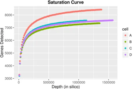
Despite the clear benefits of sequencing at sufficiently high depths, researchers would be remiss to simply sequence as much as possible. Higher sequencing depths are accompanied by higher costs, as sequencing machines can accommodate only a limited number of reads per expensive run. Moreover, it has been shown that there exists a point of diminishing returns at which continuing to increase the sequencing depth fails to yield substantially more genomic information. This is demonstrated in so-called ‘saturation curves’, which plot the number of genes detected in a given sample against an increasing number of reads. The saturation curves in Figure 2.2, generated
from the R package NOISeq [Tarazona et al., 2011], demonstrate this property using
randomly chosen samples from a real scRNA-seq data set on human prostate cell lines (described in Section 2.2).
3000 4000 5000 6000 7000 8000 0 500000 1000000 1500000
Depth (in silico)
Genes Detected cell A B C D Saturation Curve
Figure 2.2. Saturation curves of randomly chosen samples from a real scRNA-seq data set on human prostate cancer cell lines. Each curve plots the number of detected genes, defined as genes with counts greater than 3, against against sequencing depth for a cell sample. For a full description of how this plot was generated, see Tarazona et al. [2011]. As the number of reads increase, the number of genes detected also increases, but begins to taper off. This pattern is typical of both bulk and single-cell RNA-seq data.
Sequencing depth is but one piece of the puzzle when designing a scRNA-seq experiment. A second consideration of great practical interest to a researcher is the optimal number of cells to sequence. The pricing structure of the sequencing technology links these two choices of depth and replicates. As mentioned previously, the sequencing reaction occurs on the surface of a flow cell within the machine. In practice, these flow cells are composed of multiple independent lanes, with a limit to the number of reads that can be sequenced per lane. For example, the various Illumina systems can accommodate between 80 to 200 million reads per lane, depending on the choice of read length. Importantly, the largest cost of a sequencing experiment is in the price per lane. Therefore, given the financial constraints of an experiment, there exists a tradeoff between sequencing fewer cells with more reads each or more
cells each at lower depths. The optimal balance point is the question of interest, specifically in the context of detecting differential expression.
The question of optimizing the trade-off between sequencing depth and biologi-cal replicates has been asked previously of bulk RNA-seq tissues [Liu et al., 2014]. However, here the focus has changed, in keeping with the shift in context going from designing experiments for bulk samples as opposed to single cells. While bulk RNA-seq studies often limit themselves to around a dozen samples (sometimes more but often less) over two or more treatments, single-cell studies are seen to involve hun-dreds to occasionally thousands of cells that are considered biological replicates. This is partially due to the enormous reduction of labor and cost involved in isolating single cells as opposed to collecting tissue samples from whole organisms. It is also partially a necessity; a large number of cells is needed to characterize cell populations and to counter the variability of each individual cell. Hence, while in bulk RNA-seq the popular recommendation is to always obtain as many biological replicates as possible, for single-cell applications, the question remains whether there may be a saturation point beyond which more replicates is not necessary. With respect to sequencing depth, the standard is to use around 30 million reads per sample for bulk RNA-seq differential expression studies. By contrast, the number of reads per single cell, though markedly less than what is used for bulk samples, still varies substantially between studies [Stegle et al., 2015]. For example, Jaitin et al. [2014] used around
20,000 reads per cell for over 1,500 cells, while Mahata et al. [2014] sequenced an
average of 16 million reads per cell for each of around 90 cells.
There is currently no accepted rule of thumb or guide that either empirically or the-oretically instructs researchers about the optimal choice of sequencing depth and/or replicate number. Certainly, understanding this relationship has great value when designing a scRNA-seq experiment. Here, a simulation study attempts to provide guidance by investigating the effect of different combinations of sequencing depths and numbers of replicates on the detection of differential gene expression.
2.2 Procedure for Simulating scRNA-seq Data
The starting point of any simulation study is the choice of how to generate simu-lated data in a way that adequately mimics real data. Throughout this work, count data are all simulated from a zero-inflated negative binomial (ZINB) distribution, with gene-wise parameters extracted from a real scRNA-seq dataset. Specifically,
for each gene g, take ¯yg to be the mean of the non-zero counts; λg = ¯yg/
gy¯g is
then the proportion of all read counts originating from gene g, and can be
consid-ered the baseline rate of expression from gene g. The NB dispersion is calculated as
φg = (s2g−y¯g)/y¯2g, where s2g is the variance of the non-zero counts. Also recorded are
the gene-wise proportions of zero counts, pg. Parameters are sampled in gene-wise
triplets of {λg, φg, pg} to be used to generate simulated gene counts.
To introduce differential expression on a select proportion of genes, coefficients
βg reflecting the group effect are drawn as βg ∼ logNormal(2,1) for differentially
expressed genes, while coefficients for non-DE genes are set to 0. The log-linear
model for the expected count μgi of gene g in sample i is
log(μgi) =λg +xiβg+ log(mi) (2.1)
where xi indicates the group membership of the ith sample and mi is the sample i
library size included as an offset. Finally, counts are simulated as ygi ∼NB(μgi, φg),
with a proportion of counts for each gene set to zero with probability pg to mimic
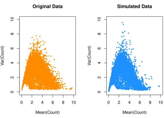
the zero-inflation prevalent in real scRNA-seq data. Figure 2.3 visually demonstrates that the mean-variance plot of the simulated data suitably mimics that of the original data from which the simulation parameters were sampled.
Real scRNA-Seq Prostate Dataset
All simulated datasets in this work are based on a real scRNA-seq dataset from an experiment involving human prostate cancer cell lines, henceforth referred to simply as the “prostate” dataset. The dataset is comprised of a treatment group containing
0 2 4 6 8 10 02468 1 0 Original Data Mean(Count) V ar(Count) 0 2 4 6 8 10 02468 1 0 Simulated Data Mean(Count) V ar(Count)
Figure 2.3. Count data from a real scRNA-seq experiment (left) provide the parameters that are used to generate simulated gene counts (right). Mean-variance plots of the simulated gene expression data suitably mimic that of the original data from which the simulation parameters were sam-pled.
65 cells in which a gene implicated in prostate cancer was knocked out, and the negative control group consisting of 76 cells to which no treatment was applied. Each cell underwent the standard process of cell capture, viability screening, and reverse-transcription. Paired-end libraries were prepared and sequenced on an Illumina HiSeq 2500 machine at an average depth of 1 million reads per cell. Following quality control, alignment, and expression quantification, the resulting count data exhibited a middle-50% of library sizes ranging from 0.85 to 1.3 million read counts. The original data comprised 36,135 sequenced genes, many of which exhibit very low expression levels.
Adopting a standard practice in the literature, only the genes that have average counts of at least 5 across all cells are considered, resulting in 10,854 remaining genes.
Sequencing Depth Resampling
In simulations that follow, sequencing depth is treated as an experimental feature whose effect on the outcome of interest is to be studied. To this end, it is necessary to vary this parameter between otherwise comparable datasets. This process is re-ferred to as “resampling” in general; specifically, “downsampling” or “subsampling” describes the process of generating datasets to lower depths.
Sequencing depth generally refers to the number of reads that are sequenced in an experiment. Recall that the library size is the total number of sequencing reads that are successfully mapped to a sample. The observed difference between raw sequencing depth and the final library size is due to a number of factors that cause a proportion of reads to be discarded. These factors include quality-control filtering, removal of
non-mRNA reads (e.g., ribosomal RNA or other artifacts), and reads that fail to map
unambiguously to the reference genome. Library sizes are therefore not equivalent to sequencing depth; however, they can reasonably act as a proportionate proxy. It has been argued by Robinson and Storey [2014] that in simulation applications that require subsampling reads in order to perform identical analyses on each subsample, it is functionally identical and substantially more computationally efficient to directly subsample the read count matrix (Table 1.1) as opposed to the raw unaligned reads. Hence, in subsequent simulations, the term ‘sequencing depth’ is used to refer to the ‘library size’ as opposed to the ‘number of raw sequencing reads’.
Mulitnomial sampling in the following manner is used to obtain samples of desired
depths D based on a set of original samples. Let yi ={yig}Gg=1 be counts for the G
genes from sample i of the original dataset, with corresponding library size Li =
gyig. Let xi = {xig}Gg=1 be the sample generated from yi with desired depth
and probabilities {yig/Li}Gg=1. This results in simulated samples xi with the same
probability distribution of gene counts as the originatingyi, but with the new depth
of Di.
2.3 Simulations
In order to study the relationship between sequencing depth and replicate number and their combined effect on detecting differential expression, datasets of varying depths and replication levels were generated from the original prostate dataset. The
depths considered for the simulation areD={0.1,0.2,0.4,0.6,0.8,1,1.2,1.4,1.6,1.8}
million reads. The number of replicates per treatment group considered are N =
{10,20,30,40,50,60}; that is, N replicates were randomly chosen from each of the
treatment and control groups. 50 datasets were generated for each combination of
D× N (Table 2.1). The R package edgeR was applied to each simulated dataset
to test for differentially expressed genes. The genes considered ‘truly’ DE are those
testing significant in the most ‘robust’ simulation scenario, i.e., the dataset with the
highest sequencing depth (D= 1.8 million reads) and replicates per group (N = 60),
at a false discovery rate (FDR) cutoff of 0.001. Using these ‘true’ DE genes as the gold standard for comparison, the statistical power of each experimental design may be calculated as the number of true DE genes that are also detected as DE (true positives), divided by the total number of true DE genes (positives).
Figure 2.4 (top) shows the statistical power to detect DE genes as a function of depth and replicates. Increasing the number of replicates substantially and consis-tently increases statistical power. By contrast, increasing the sequencing depth has a much smaller effect on power, and plateaus off after a point. Figure 2.4 (bottom) depicts the number of differentially expressed (DE) genes detected for the various combinations of sequencing depths and replicates per group. Consistently more DE genes are called as the number of replicates increases, particularly at higher sequenc-ing depths. Increassequenc-ing the sequencsequenc-ing depth has little to no effect on callsequenc-ing DE genes
Table 2.1
Simulated datasets are generated from the real prostate dataset, by
ran-domly selecting N replicates per experimental group in the real data,
and resampling counts to the desired depth D. 50 datasets are simulated
for each combination of D×N, and edgeR is applied to obtain lists of
differentially expressed genes detected in each setting.
Depths (D)
0.1M 0.2M ... 1.8M
Reps per Group (N)
10
20 ×50
... 60
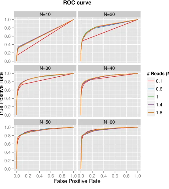
at lower replication levels, but has increasing effects at higher replication levels. The ROC curves in Figure 2.5 depict the effect of sequencing depth on the accuracy of DE testing for each level of replication. At lower replication levels, increasing the number of reads has some effect on accuracy, most notably moving away from the very lowest depths. However, as replication levels increase, more reads hardly contributes at all to increasing the accuracy of the test. In general, the area under the ROC curve improves as more replicates are included.
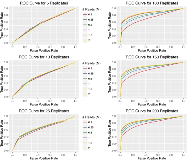
The results depicted in Figures 2.4 and 2.5 are limited in the maximum num-ber of replicates per group that they are able to show, as they are based on direct subsampling of a real prostate dataset consisting of only 64 replicates for its smaller experimental group. The effects of greater sample sizes may be observed through gen-erating synthetic data containing higher replicate numbers. This was accomplished by simulating datasets based on parameters extracted from the same human prostate scRNA-seq data (as described in Section 2.2). The intended effect was to mimic the real data in distributional parameters, but with group replicate numbers ranging from
N=10 N=20 N=30 N=40 N=50 N=60 0.0 0.2 0.4 0.6 0.8 1.0 0.0 0.2 0.4 0.6 0.8 1.0 0.0 0.2 0.4 0.6 0.8 1.0 0.0 0.2 0.4 0.6 0.8 1.0 0.0 0.2 0.4 0.6 0.8 1.0 False Positive Rate
T rue P ositiv e Rate # Reads (M) 0.1 0.6 1 1.4 1.8 ROC curve
Figure 2.5. Results from datasets subsampled from the real prostate data, to varying sequencing depths and replicates per group. A separate ROC curve is depicted for each of the considered replication levels per group, and individual lines represent sequencing depths.
20 to 200. As expected, as the number of replicates per group continue to increase, diminishing returns are observed in both the number of DE genes detected as well as the statistical power to call true DE genes (Figure 2.6), particularly as the number of replicates per group reaches into the hundreds. ROC curves for the synthetic data
(Figure 2.7) demonstrate similar patterns to those in Figure 2.5, in that higher repli-cates consistently lead to higher areas under the curve, and increasing sequencing depth has little positive effect beyond the lowest depths.
Observations made here are consistent with what has been suggested previously with Liu et al. [2014] in bulk RNA-seq studies; that is, the number of biological replicates has a markedly more positive effect than sequencing more deeply. This said, for both variables, more is always better, but only up to a point.
2.4 Guiding the Choice of Optimal Experimental Design
Recommendations as to the choice of sequencing depth and replicate number may offer general guidelines in the way of experimental design. However, the real practi-cal interest for researchers is in the ability to make experiment-specific decisions that are informed by the real or expected variability in their data, as well as constraints such as desired statistical power and budgetary limits. As part of this investigation,
an interactive tool was implemented in a Shiny web application called scDesignApp,
which may be accessed at https://fayezor.shinyapps.io/scDesignApp/. It is
accompanied by an associated R package called scDesign, which may be installed
from GitHub at https://github.com/fayezor/scDesign. Given pilot data,
typi-cally based on real data, this tool calculates statistical power and estimates costs for each of a user-specified range of experimental designs.
The general workflow for the implementation of the scDesign tool is as follows.
First, the user provides a pilot dataset from which parameters will be estimated in subsequent calculations. These pilot data may be either a small-scale portion of the planned experiment or related prototype data from similar previous experiments. Recommendations for pilot data best practices are proposed in Section 2.4.3. To compare a variety of hypothetical experimental designs, users must specify a range of sequencing depths and a range of replication levels to be considered. Each com-bination of depth and replication level constitutes an experimental design. Other
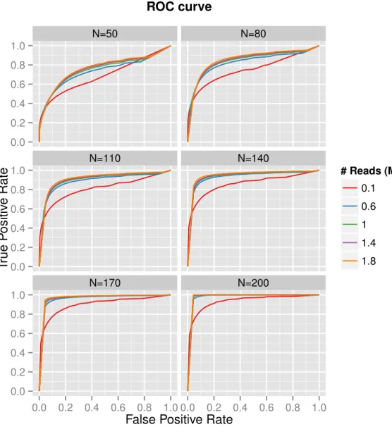
N=50 N=80 N=110 N=140 N=170 N=200 0.0 0.2 0.4 0.6 0.8 1.0 0.0 0.2 0.4 0.6 0.8 1.0 0.0 0.2 0.4 0.6 0.8 1.0 0.0 0.2 0.4 0.6 0.8 1.0 0.0 0.2 0.4 0.6 0.8 1.0 False Positive Rate
T rue P ositiv e Rate # Reads (M) 0.1 0.6 1 1.4 1.8 ROC curve
Figure 2.7. ROC curves for each of the considered replicate numbers per group. Lines in each curve represent the sequencing depth. Plots were generated from simulated data generated using distributional parameters extracted from the human prostate scRNA-seq dataset.
inputs from the user may include the desired statistical power, budget constraint, false-discovery rate (FDR) to be controlled, and anticipated cost parameters.
Gene-specific parameters are estimated from the user-provided pilot data, and statistical power is calculated for each experimental design. Statistical power is
ad-dressed in two ways. First, an empirical power calculation is performed by simulating datasets for each design and recording the observed levels of statistical power ob-tained. Second, a theoretical method implements the power-estimation procedure of Bi and Liu [2016]. Both statistical power calculation methods are described in Section 2.4.1 in greater detail. Finally, the cost of each experimental design is also projected, based on the formula and default cost assumptions provided in Section 2.4.2.
2.4.1 Statistical Power Calculation
The utility of the interactive tool comes from employing a dataset that is either a subset of or representative of a full experiment, and obtaining estimates of what the statistical power might be to detect differential expression if the researcher were to carry out a full experiment of a specified size. It is therefore important to choose with care the method of experiment-wide statistical power estimation.
Several methods exist for RNA-seq statistical power calculations that are per-formed on a gene-by-gene basis, with varying assumptions about the distribution of the true underlying expression values. For example, Fang and Cui [2011] propose a formula based on the Wald test for single-gene differential expression analysis, while treating the data as Poisson. Hart et al. [2013] treat the data as negative binomial and derive a formula based on a score test, highlighting the relationship between technical and biological variability, and using empirical justifications for how to choose certain
parameters of the formula. Busby et al. [2013] uses a non-central t-distribution to
approximate the statistical power of an experiment, arguing that a normal approxi-mation is reasonable for RNA-seq data; however, such justifications are generally not accepted in the general literature, as RNA-seq count data are often known to have distributions too skewed to be modeled as normal.
What is of most interest, however, is not merely the statistical power of a single gene, but of experiment-wide power over the tens of thousands of genes measured in an RNA-seq experiment. Single gene statistical power calculations are often accompanied
by suggestions for how to pool per-gene powers over an experiment; typically this involves taking the average, with or without allowing parameters to vary between genes. However, in situations involving many simultaneous tests as with RNA-seq, it is necessary to account for this multiple testing using error criterion such as the false discovery rate (FDR) [Benjamini and Hochberg, 1995].
One procedure for calculating experiment-wide statistical power while controlling for FDR is proposed in Li et al. [2013a], consisting of a single gene formula for com-puting statistical power based on several test statistics, and an extension of that formula to incorporate FDR control. However, the procedure is based on a Poisson distribution, which is inappropriate for the overdispersion present in RNA-seq exper-iments involving many biological replicates. The authors try to address this in Li et al. [2013b] by assuming a negative binomial distribution for the expression counts,
and using a statistical power calculation based on the exact test as used in edgeR
for testing differential expression between two groups. However, several features of the procedure render it extremely conservative; for example, statistical power is com-puted by setting the fold change parameter to be the minimum fold change observed across all genes deemed differentially expressed, and similarly setting the dispersion to the maximum observed. This likely limits the practicality of the procedure.
It is evident that experiment-wide statistical power considerations for RNA-seq data while controlling FDR is underdeveloped. Reflecting on the microarray litera-ture, Liu and Hwang [2007] calculate statistical power at a specified FDR level by
finding the rejection region for the test procedure. The authors use t-tests to model
microarray data. The recent Bi and Liu [2016] takes the machinery of Liu and Hwang
[2007] and makes it applicable to RNA-seq data by applying the voommethod of the
limma package to first transform the count data into normalized log-counts. This circumvents the direct use of the negative binomial distribution, for which there exist no analytical relationships between statistical power and sample size, as there are no closed-form solutions for the maximum likelihood estimate of the NB dispersion. Due to the applicability of Bi and Liu [2016] to RNA-seq data, its control of FDR to
account for multiple testing, and its avoidance of computationally-heavy simulations, this procedure is implemented for the theoretical statistical power calculation in our experimental design tool. The details of the procedure are as follows, as originally described in Liu and Hwang [2007] and Bi and Liu [2016].
Theoretical Calculation of Statistical Power
Let H0 and H1 be indicators that the null or the alternative hypothesis is true,
respectively; let Γ be the rejection region of a given test statistic T; and let π0 be
the assumed proportion of true nulls. Table 2.2, originally shown in Benjamini and
Hochberg [1995], is popularly used to categorize the different outcomes of testing G
hypotheses.
Table 2.2
Table of outcomes when testing G simultaneous hypotheses, π0 of which
are true nulls.
Declared non-significant Declared significant Total
H0 is true U V π0·G
H1 is true T S (1−π0)·G
Total G−R R G
The false discovery rate (FDR) is defined as the expected proportion of false positives among the rejected hypotheses Benjamini and Hochberg [1995]. That is,
F DR=E V R R >0 P(R >0). (2.2)
Storey [2003] offered a slight modification of this to the positive false discovery rate,
defined as pF DR=E V R R >0 . (2.3)
Since it may safely be assumed in genomic studies that there will be at least one
rejection, i.e. that R > 0, pFDR and FDR will be used interchangeably here. By
Bayes rule, (2.3) can be written1as
P(H0|T ∈Γ) = P(T ∈Γ|H0)·π0
P(T ∈Γ|H0)·π0+P(T ∈Γ|H1)·(1−π0) (2.4)
In order to control FDR at a given level α, setting equation (2.4) to be less than or
equal to α yields the following relationship with some simple algebra.
α 1−α 1−π0 π0 ≥ P(T ∈Γ|H0) P(T ∈Γ|H1) (2.5)
On the right-hand side, Type I error is in the numerator and statistical power is in the denominator. The task is to find the rejection region Γ so that equation (2.5) is
satisfied, hence controlling FDR at level α; statistical power may be computed once
the rejection region is known.
The original application of Liu and Hwang [2007] was intended for microarrays,
in which the data were appropriately assumed to be normal and t-tests could be
applied for two-sample comparisons. However, the method is not directly applicable to commonly applied tests for RNA-seq data involving a negative binomial distribution,
as there are no closed-form solutions for calculating P(T ∈ Γ|H0) and P(T ∈Γ|H1).
As mentioned earlier, Bi and Liu [2016] extended the method to be used for RNA-seq data by first transforming the data to a normalized log-counts per million (log-cpm)
value, as part of the method calledvoomimplemented in theRpackage limma(Linear
1The Bayesian interpretation of the pFDR (2.3) is detailed and proven in Theorem 1 of Storey [2003]. Briefly, givenGidentical tests of the null hypothesisH0 with accompanying test statisticsT1, ...TG
and a given rejection region Γ,pF DRmay be rewritten as
pF DR=E V(Γ) R(Γ) R(Γ) ,
whereV(Γ) = #{null Ti|Ti∈Γ}andR(Γ) = #{Ti|Ti ∈Γ}. P(H0|T ∈Γ) represents the probability
of a false positive, given a significant test statistic. For the case when G= 1, V(Γ)/R(Γ) must be either 0 or 1, so it easily follows thatpF DR=P(H0|T ∈Γ). Storey [2003] show, with proof, that this result is the same for whenG >1.
Models for Microarray Data). This approach allows for the derivation of a t-test based test statistic formula that can subsequently be used in the application of the original method as before.
In a two-sample comparison, where the interest is to find differentially expressed
genes between two experimental groups, the hypothesis to test for each gene g is
H0g :μg1 =μg2 (2.6)
H1g :μg1 =μg2, (2.7)
where μg1 and μg2 are means of the normalized counts in each group. The t-test
statistic for geneg is
Tg = Δg sg 1 n1 + 1 n2 , (2.8)
where Δg is the scaled effect size, defined as the weighted mean difference of log-cpm
values between groups, and sg is the pooled standard deviation. To accommodate
the practical situation where genes may exhibit different parameters, assume that the
effect size Δg for each gene follows a normal distribution
Δg ∼N(μΔ, σΔ2), denoted by π1(Δg), (2.9)
and the variance of log-cpm values follows an inverse gamma distribution
σ2g ∼InvGamma(a, b), denoted by π2(σg). (2.10)
The average statistical power across all genes may be written as an integral over these distributions,
P(T ∈Γ|H1) =
P(T ∈Γ|H1,Δg, σg)π1(Δg)π2(σg)dΔgdσg. (2.11)
α 1−α 1−π0 π0 ≥ P(T ∈Γ|H0) P(T ∈Γ|H1) = P(T ∈Γ|H0) P(T ∈Γ|H1,Δg, σg)π1(Δg)π2(σg)dΔgdσg = P(|Tg|> c|H0) P(|Tg|> c|H1,Δg, σg)π1(Δg)π2(σg)dΔgdσg (2.12)
Using the knowledge that Tg is distributed as a central t-distribution under the null
and a non-central t-distribution under H1, the denominator in (2.12) is
1− Tn1+n2−2(c|θg)π1(Δg)π2(σg)dΔgdσg + Tn1+n2−2(−c|θg)π1(Δg)π2(σg)dΔgdσg, (2.13)
where θg is the non-centrality parameter defined as
θg = Δg σg 1 n1 + 1 n2 , (2.14)
and the numerator in (2.12) equals
P(T ∈Γ|H0) =P(|Tg|> c|H0) = 2·Tn1+n2−2(−c). (2.15)
Once the critical value c has been obtained which satisfies the relationship in (2.12)
for a given level α and proportion of nulls π0, statistical power may be calculated
from equation (2.13) for a specific sample size.
The practical implementation of this method based on pilot data is achieved by first simulating a scRNA-seq count dataset as described in Section 2.2, with simula-tion parameters drawn empirically from the user-submitted pilot data. These counts
are normalized to log-cpm by applying voom/limma as previously described, and are
used to estimate the hyperparametersμΔ, σΔ, a, and bwhich characterizeπ1(Δg) and
π2(σg). These characterized distributions can finally be used to solve the integrals
Empirical Calculation of Statistical Power
In order to double-check how reasonable the theoretical statistical power
calcu-lation is, scDesign also implements an empirical power calculation based fully on
simulations. This is done by first extrapolating the given pilot data to each desired experimental design setting. That is, parameters drawn from the pilot data are used to simulate a new dataset with the desired sequencing depth and number of repli-cates per group and containing a known set of differentially expressed genes. The
R package edgeR is then applied to test for differential expression, and the resulting
adjusted p-values are used to obtain the statistical power. Specifically, statistical power is calculated as the number of genes determined significant at a specified FDR that are truly DE (true positives), divided by the total number of truly DE genes in the simulated dataset (positives). This is repeated a number of times, and the average of statistical powers in each iteration is taken to be the empirical calculation of statistical power for the given experimental design. Figure 2.8 shows that for a given depth, the theoretical and empirical estimates of statistical power are similar, with empirical calculations being slightly more conservative. While a statistical power of 0.8 is a typical standard target for experiments, such levels of power are harder to achieve for scRNA-seq data, which are often zero-inflated with higher variability among replicates even of the same treatment group.
A few remarks bear noting. First, the empirical statistical power calculation in-evitably reflects the power of the method chosen to test differential expression, in
this case edgeR. Other methods, for example DESeq2, SCDE, or limma, among others,
will likely yield different power estimates. edgeR was chosen for its useability on
data simulated to mimic scRNA-seq data; other attempted methods either yielded substantially lower statistical power or were computationally intractable for large numbers of replicates. Second, the empirical power calculation is significantly more computationally intensive than the theoretical power calculation, as it involves
tiplexing, and equipment. Attolini et al. [2015] incorporate read-specific costs in the following equation:
cost = (c0×N) + (c1×2rDN), (2.17)
where N is the number of samples, each associated with a fixed cost c0. 2r denotes
the read length for paired-end experiments, D the number of reads per sample, and
c1 the cost per read.
Building on (2.17) to incorporate costs specific to single-cell experimental designs,
the following cost function is proposed. Let N, as before, denote the number of
samples, in this case individual cells, with a per-cell cost of ccell. These cells are
captured onto plates which hold a default 96 cells at a time, at a per-plate cost of
cplate. This may be adjusted to a higher number of cells per plate, which may soon
increase to as many as 800 cells per plate, as high-throughput cell capture protocols become more widely available. In addition to cell and plate costs, there are also
per-lane costs clane, where each lane can accommodate a maximum number of reads,
max. Finally, there may be other miscellaneous costs to be captured in cf ixed.
cost = (ccell×N) + (cplate× N/96) + (clane× N D/max) +cf ixed (2.18)
A practical adjustment to the cost function is to account for inefficiencies in the capturing of cells and the sequencing of reads. That is, there may be some proportion of cells on the 96-well capture plates that are captured incorrectly or do not pass a
viability screen. Ifpcapturedenotes the capture efficiency, an input ofN cells will result
in N ×pcapture cells being used in the analysis. In addition, there is typically some
proportion of sequenced reads that do not get aligned and are hence not quantified; reasons for this include the filtering of reads that do not pass quality control, am-biguously mapping reads, or reads from artifacts such as rRNA rather than genomic
amount of sequenced reads that align successfully and thus quantified. The following cost function incorporates these adjustments.
cost = (ccell×N) + (cplate× N/96×pcapture) (2.19)
+ (clane × N D/max×psample×pseq+cf ixed
The costs of cell, plate, and lane may be chosen with real experiments as a guide. Table 2.3 presents some typical costs associated with various stages of the scRNA-seq workflow, from cell capture to sequencing; these numbers are based on the actual costs of the prostate data described in Section 2.2. Per-cell costs may include kits for cDNA dilution and library prep; per-plate costs may cover plate reagents as well as the plate itself; per-lane costs comprise the costs of the sequencing itself, depending on read length and paired- or single-end sequencing; and fixed costs may include
items such as assay tubes, viability kits, and labor. The scDesign tool allows for
the specification of the following default parameters: costs per cell, plate, and lane are respectively $1200, $20, and $2000; fixed costs per experiment are $1200; and the maximum number of reads per lane is 96 million. Again, these values are based on the observed costs of the prostate dataset in particular, but may vary widely across different cell types, experimental platforms, and sample preparation protocols.
2.4.3 Pilot Data
Researchers often elect to first sequence a handful of replicates at a lower depth to get a sense of their data before committing to an expensive full experiment. The utility of our tool is that it requires only the pilot data to estimate what the statistical power would be in a full imagined experiment; it does so by taking parameters learned from the pilot dataset to extrapolate the data to “full” size, and using the full data as a basis for calculations. A natural question might be what is the effect of the size of the pilot data on the ability of the extrapolations to accurately recover properties of the full dataset.
Table 2.3
Some typical costs associated with various stages of the scRNA-seq work-flow, from cell capture to sequencing; these numbers are based on the actual costs of the prostate data described in Section 2.2.
Item Cost
Cell Isolation
96-well plates $700/ea
Instrument reagents $440/plate
Viability kit $400
Library Prep Library prep kit $12.50/cell
Other (reagents, tubes) $305
Sequencing HiSeq Rapid PE 100bp $1990/lane
Multiplexing $300/two lanes
To investigate this, a full-size dataset was simulated with the approach described in Section 2.2, and relying on parameters taken from the prostate scRNA-seq data. The experimental design of these full data consist of two hundred replicates per group at depths of two million. There are ten thousand genes, one thousand of which
exhibit true differential expression. edgeR was applied to detect DE genes, with
results serving as a baseline for comparison in later analyses of pilot datasets; 647 genes were detected as DE, with a true positive rate (TPR) of 0.625 and false positive rate (FPR) of 0.002.
Pilot datasets were obtained from the full-sized dataset, by down-sampling to a range of smaller experimental designs in a similar fashion as Section 2.2. Specifically,
the number of replicates per treatment group considered areN ={5,10,25,50,10,150,
200}, and the depths considered are D = {0.1,0.25,0.5,1,1.5,2} million reads. 20
datasets were generated for each combination of N ×D. To extrapolate each pilot
dataset back to full size while keeping any original differential expression patterns, the simulation procedure of Section 2.2 was adapted to allow the estimation of