Robust variable selection in partially varying coefficient
single-index model
Huiming Zhua, Zhike Lva,∗, Keming Yub, Chao Denga
aCollege of Business Administration, Hunan University, Changsha, 410082, PR China bDepartment of Mathematical Sciences, Brunel University, London UB8 3PH, UK
Abstract
By combining basis function approximations and smoothly clipped absolute deviation (SCAD) penalty, this paper proposes a robust variable selection procedure for partially varying coefficient single-index model based on modal regression. The proposed procedure simultaneously selects significant variables in the parametric components and the nonparametric components. With appropriate selection of the tuning parameters, we establish the theoretical properties of our procedure, including consistency in variable selection and the oracle property in estimation. Furthermore, we also discuss the bandwidth selection and propose a modified expectation-maximisation (EM)-type algorithm for the proposed estimation procedure. The finite sample properties of the proposed estimators are illustrated by some simulation examples. Keywords: Variable selection; Spline approximation; Modal regression; SCAD; Oracle property
1. Introduction
Partially varying coefficient single-index model (PVCSIM) combines naturally the advantages of both the single-index models and the varying coefficient models. Ever since Wong, Ip, and Zhang (2008) proposed the PVCSIM, studies in this class of model have raised the great interest of research in Statistics field. We formulate a PVCSIM as
Y =ZTθ(U) +g(XTβ) +ε, (1.1) where Y is a response variable, X and Z are of dimensions p×1 vectors and q×1 vectors, θ(·) = (θ1(·), ..., θq(·))T is a vector of unknown function,β = (β1, ..., βp)T is a vector of unknown parameters,g(·)
is an unknown link function, and εis random error with mean zero. Due to the curse of dimensionality, we assume, for simplicity, that U is univariate. And we also assume that kβk = 1 and sigh(β1) = 1 to
ensure identifiability, wherek · kdenotes the Euclidean metric.
Model (1.1) is quite flexible enough to cover a variety of existing statistical models. For example, if g(·) = 0, it reduces to the standard varying-coefficient model. When θ(·) is an unknown constant
parameter, then model (1.1) is a partially linear single-index model (Wang, Xue & Chong, 2010; Wang & Wu, 2013). In addition, model (1.1) becomes the standard single-index model whenZ= 0 orθ(·) = 0 (Wu, Yu & Yu, 2010). Due to its flexibility and generality, model (1.1) has gained much attention in recent years. Wang and Xue (2011) developed a stepwise approach to obtain asymptotic normality estimators of the varying-coefficient vector and the parametric vector. Huang and Zhang (2010) constructed the confidence region for the parameter β in model (1.1) based on the empirical likelihood technique. While Huang (2011) used the empirical likelihood method to study the confidence regions of the varying-coefficient parts. Huang, Lin, Feng and Pang (2013) proposed a class of efficient penalized estimating equations to estimate the index parametric components in the PVCSIM. Feng and Xue (2013) also considered the problem of variable selection in the PVCSIM. However, the aforementioned existing researches were mainly built on either the least-square or empirical likelihood method, which are expected to be very sensitive to the outliers and its efficiency may be significantly decreased for many commonly used non-normal errors. Recently, Yao, Lindsay and Li (2012) proposed a new estimation approach based on a local modal regression for the nonparametric model. Then, Zhang, Zhao and Liu (2013) and Zhao, Zhang, Liu and Lv (2014) investigated the partially linear varying coefficient model based on modal regression, respectively. And Liu, Zhang, Zhao and Lv (2013) developed a new robust and efficient estimation procedure based on local modal regression for single index models. A distinguishing characteristic of their method is that it introduces an additional tuning parameter which is automatically selected using the observed data to achieve both robustness and efficiency of the resulting estimate. Namely, their method is not only robust when there are outliers or the error distribution is heavy-tail, but as asymptotically efficient as the ordinary least-square-based estimator when the data include no outliers and the error distribution is a Gaussian distribution. Due to its nice property, it has attracted increasing attention. Here, we extend the modal regression approach to the model (1.1).
Variable selection is a crucial issue in regression analysis. In practice, a number of variables are available for inclusion in an initial analysis, but many of them may not be significant and should be excluded from the final model to increase the accuracy of prediction. Traditional variable selection methods such as stepwise regression and best subset selection are computationally infeasible when the number of predictors is large. Therefore, various shrinkage methods such as the LASSO (Tibshirani 1996), the adaptive LASSO (Zou 2006) and the SCAD (Fan & Li 2001) have gained much attention in recent years. However, the LASSO is known to be near mini-max optimal as well as consistent under certain regularity conditions, Zou (2006) showed that it falls short of attaining the oracle property. By this property, an estimator estimates a zero coefficient exactly as zero with probability approaching one, while still being asymptotically normal for the non-zero coefficients in large samples. In this respect, the LASSO is inferior to the SCAD estimator which possesses the oracle property. So in the present paper, we prefer the SCAD of Fan and Li (2001) since it simultaneously satisfies the mathematical conditions for unbiasedness, sparsity, and continuity. More detail can be found in Fan and Li (2001). Since the SCAD was proposed, there has been a large number of literature focused on its applications in many important nonparametric and semiparametric models.
In this paper, we investigated the variable selection for the varying coefficient function θ(·) and the unknown parametric index β in model (1.1) based on modal regression. By combining the basis func-tion approximate and the SCAD penalty, we develop a variable selecfunc-tion procedure for PVCSIM. More specifically, we first use the B-spline functions to approximate the unknown coefficient functions and link function in model (1.1). And then combine with the restraintkβk= 1 to construct the penalized estima-tion funcestima-tion for PVCSIM based on modal regression. Under certain regularity condiestima-tions, we are able to establish this variable selection procedure is consistent, and the estimators have oracle property. More-over, a modified version of a modal expectation-maximisation (MEM) algorithm is proposed to obtain the solutions for the object function. Some simulation studies show that, when data is contaminated by outliers, the proposed variable selection procedure can perform well in finite samples.
The layout of the remainder of the paper is as follows. In Section 2, following the idea of the modal regression approach, we propose the regularized estimation produce using basis expansion and the SCAD penalty function. Then, Under some regularity conditions, we establish some theoretical properties of the proposed variable selection procedure. We describe the detail of bandwidth selection and propose a modified MEM algorithm. In addition, we give the method of choosing the tuning parameters in Section 3. In Section 4, we conduct some simulation studies to examine the finite sample performance of the proposed procedures. Finally, in section 5 we conclude the paper. All the regularity conditions and the technical proofs are relegated to Appendix.
2. Estimation and variable selection procedure
As a measure of centre, the median and mode have the common advantage of robustness, when there exist outliers. Furthermore, since the modal regression focuses on the relationship between the majority data points and summaries the “most likely”conditional values, it can provide more meaningful point prediction than the mean regression when the error density is skewed. Suppose that{(Yi, Xi, Zi, Ui), i=
1, ..., n} is an i.i.d. sample from model (1.1). Then following the method of Yao, Lindsay and Li (2012), the robust modal estimate of the PVCSIM is to maximize
1 n n X i=1 φh Yi−ZiTθ(Ui)−g(XiTβ) , (2.1)
where φh(t) = h−1φ(t/h), φ(t) is a kernel density function, and the choice ofφ(·) is not very important. his a bandwidth. For ease of computation, we use the standard normal density for φ(t) throughout the present article.
Remark 1. The choice of kernel is not very important because it is possible to obtain estimators with somewhat improved asymptotic properties by using different kernels (see, e.g., Eddy, 1980; Romano, 1988). For the simplicity of the calculation, we use the Gaussian density forφ(t).
2.1. Spline-based estimation
Since θ(·) and g(·) are unknown functions in (2.1), here, we use polynomial splines to approximate it. More specifically, let B1(u) = (B11(u), ..., B1L1(u))
T and B
2(t) = (B21(t), ..., B1L2(t))
B-spline basis functions with the order of M1+ 1 and M2 + 1, respectively, where L1 = K1 +M1 + 1
and L2 =K2+M2+ 1, with K1 andK2 are the number of interior knots, Thenθj(u) and g(t) can be
approximated by
θj(u)≈B1(u)Tγj, j= 1, ..., q. and g(t)≈B2(t)Tη.
Then, we can obtain ˆγ, ˆη and ˆβ by maximizing 1 n n X i=1 φh Yi−WiTγ−B2(XiTβ) Tη, (2.2)
whereWi=Iq⊗B1(Ui)·Zi withIq is aq×qidentity matrix, andγ= (γ1T, ..., γTq)T.
2.2. Variable selection for PVCSIM
In this subsection, our main goal is to find zero components (i.e., θj(·) = 0 andβs= 0) in PVCSIM.
Thus, we define the following semiparametric penalized estimation for PVCSIM based on modal regression as L(γ, η, β)≡ 1 n n X i=1 φh Yi−WiTγ−B2(XiTβ) T η− q X j=1 pλ1j(kγjkH)− p X s=1 pλ2s(|βs|), (2.3) where pλ1j and pλ2s are two penalized parameters for the jth varying coefficient function and the sth parameter component, respectively. kγjkH = (γjTHγj)1/2withH =
R
B1(u)B1(u)Tdu.
Remark 2. Formulation (2.3) includes many popular variable selection methods, for example, the Lasso (Tibshirani 1996) uses theL1penalty withpλ1(k · k) =λ1k · k. Bridge regression (Frank & Friedman 1993)
uses theLq penalty withpλ1(k · k) =λ1k · k
q. When 0< q <1 theL
q penalty is concave over (0,∞) and
nondifferentiable at zero. Fan and Li (2001) proposed the use of the SCAD penalty defined by its first derivative as p0λ(x) =λ n I(x≤λ) +(aλ−x)+ (a−λ) I(x > λ) o ,
for some a >2. The SCAD penalty is a spline function on an interval near zero and constant outside, so that it can shrink small value of an estimate to zero while having no impact on a large one. As illustrated in Fan and Li (2001), this penalty function satisfies three requirements for variable selection, namely, asymptotic unbiasedness, sparsity and continuity of the estimated parameters. Therefore, we only focus on the SCAD penalty function throughout of this paper.
Recalling that we assume that kβk = 1, this means that true value of β is a boundary point on the unit sphere, which causes some difficulty since g(XiTβ) does not have a derivative at the point β. To solve this problem, we suggest the popularly used “delete-one-component” method proposed by Yu and Rupper (2002). The detail is as follows, without loss of generality, we assume that the true parameterβ
has a positive componentβ1 (otherwise, consider -β1). Forβ = (β1, ..., βp)T, let β(1) = (β2, ..., βp)T be a
(p−1)-dimensional parameter vector after deleting the 1th componentβ1 in β. Then, we can rewrite
β =β(β(1)) = (1− kβ(1)k2)1/2, β 2, ..., βp
T
The true parameterβ(1)satisfies the constraintkβ(1)k<1. Thus,β is infinitely differential in a
neighbor-hood ofβ(1). Let e
α= (γT, ηT, βT)T andα= (γT, ηT, β(1)T)T, and the Jacobian matrix is
Jβ(1)=∂β/∂β(1)= (κ1, ..., κp)T, (2.4)
where κs (1 < s ≤ p) is a (p−1)-dimensional unit vector with sth component 1, and κ1 = −(1−
kβ(1)k2)1/2β(1).
By this reparametrization, and note that α is one dimension lower thatαe, so the objective function (2.3) is transformed to L(α)≡ 1 n n X i=1 φh Yi−WiTγ−B2(XiTβ(β (1)))Tη − q X j=1 pλ1j(kγjkH)− p−1 X s=1 pλ2s(|β (1) s |), (2.5)
In order to facilitate use, we note that maximizing the objective function (2.5) is equivalent to minimizing
e L(α)≡ −1 n n X i=1 φh Yi−WiTγ−B2(XiTβ(β (1)))Tη+ q X j=1 pλ1j(kγjkH) + p−1 X s=1 pλ2s(|β (1) s |), (2.6)
Let ˆγ, ˆη and ˆβ(1) be the solution by minimizing (2.6). Thus, the estimators ofβ,θ
j(u) and g(t) can be obtained by ˆ β= ( q 1− kβˆ(1)k2,βˆ(1)T)T, ˆg(t) =B 2(t)Tηˆ and ˆθj(u) =B1(u)Tˆγj, j= 1, ..., q. (2.7)
Next, we study the theoretical property of the proposed penalized estimators. We first introduce some notations. Let β0 and θ0(·) be the true values of β and θ(·), respectively. Without loss of generality,
we assume that β0s = 0 for s = d2+ 1, ..., p, and β0s 6= 0 for s = 1, ..., d2. Similarly, we assume that
θ0j(·) = 0 for j =d1+ 1, ..., q, and θ0j(·)6= 0 for j = 1, ..., d1. In addition, F(u, t, z, h) =E[φ00h(ε)|U = u, XTβ =t, Z =z] and G(u, t, z, h) =E[φ0
h(ε)2|U =u, XTβ=t, Z=z]. The following theorem gives the
consistency of the proposed penalized estimators.
Theorem 1Suppose that the regularity conditions C1∼C9 in the Appendix hold and the number of knots
K=Op(n1/(2r+1)), Then we have
(a) kβˆ−β0k=Op(K−r+an),
(b) kθˆj(·)−θ0j(·)k=Op(K−r+an), j= 1, ..., q,
wherean= maxj,s{|p0λ1j(|β0j|)|,|p 0
λ2s(kγ0skH)|:β0j 6= 0, γ0s6= 0}, andr is defined in the Appendix.
Remark 3. Theorem 1 implies that, the rates of convergence of the proposed penalized estimators depend on λ1j, λ2s and K. So the rates of convergence of the proposed penalized estimators can be
further improved to kβˆ−β0k = Op(K−r) and kθˆj(·)−θ0j(·)k = Op(K−r) if λmax → 0, then an = 0.
Furthermore, under some conditions, we show that such consistent estimators must possess the sparsity property, which is stated as follows.
andKrλ
min→ ∞asn→ ∞. Then with probability tending to 1, βˆ andθˆj(·)satisfy
(a) ˆβs= 0, s=d2+ 1, ..., p,
(b) ˆθj(·) = 0, j=d1+ 1, ..., q,
whereλmax= maxj,s(λ1j, λ2s)andλmin= minj,s(λ1j, λ2s).
Next, we show that the estimators for nonzero coefficients in the parametric components have the same asymptotic distribution as that based on the correct submodel. To demonstrate this, we require further notations in order to present the oracle properties of the resulting estimators. Defineγ0A= (γ01T, ..., γ0Td1)
T
and β0A = (β01, ..., β0d2)
T to be true values of γ
A and βA, respectively. Corresponding covariates are denoted by WiA and GiA = g0(XiTAβ(β (1) 0A))J T β0(1)AXiA. In addition, let Σ = E(G(U, T, Z, h)GeAGe T A) and Σ1 = E(F(U, T, Z, h)GeAGeTA) withGeA =GA−ΦTΛ−1WA, where Φ = E(F(U, T, Z, h)WAGTA) and Λ = E(F(U, T, Z, h)WAWAT).
Theorem 3Suppose that the regularity conditions C1∼C9 in the Appendix hold, √ n( ˆβA−β0A) D −→N(0, Jβ(1) 0A Σ−11ΣΣ−11JT β0(1)A), (2.8)
where “−→” represents the convergence in distribution.D
3. Bandwidth selection and estimation algorithm
The purpose of this section is twofold. we will first discuss the selection of bandwidth in theory. Then, we will discuss a modified MEM algorithm for the PVCSIM.
3.1. Optimal bandwidth
For the sake of simplicity, we assume that the error variable independent of U,X and Z, then based on (2.8) and the asymptotic variance of the least-square B-spline estimator(LSBS) given in Feng and Xue (2013), we can show that the ratio of the asymptotic variance of the modal regression (MR) estimator to that of the LSBS estimator is given by
R(h),G(h)F −2(h)
σ2 , (3.1)
where G(h) =E[φ0h(ε)]2, F(h) = E[φ00h(ε)]2 and σ2 =E(ε2). Obviously, the ratioR(h) only depends on
h, and it plays a key role in efficiency and robustness of estimators. So the ideal choice ofhis
hopt= arg min
h R(h) = arg minh G(h)F
−2(h). (3.2)
From above, we can see that hopt does not depend on n and only depends on the conditional error
3.2. Algorithm
In this subsection, we extend the local quadratic algorithm(LQA, Fan & Li 2001) and the MEM algorithm (Li, Ray, & Lindsay, 2007) to maximize (2.5) in Section 2.
Since the SCAD penalty is irregular at the origin, maximizing (2.5) directly may be difficult. Here, we use an iterative algorithm based on the local quadratic approximation of the penalty functionpλ(·) as in
Fan and Li (2001). More specifically, in a neighborhood of a given nonzero u0, an approximation of the
penalty function at valueu0can be given by
pλ(|u|)≈pλ(|u0|) + 1 2 p0λ(|u0|) |u0| (u2−u20).
Therefore, for the given initialφ(0)s (φs=β
(1)
s ) with|φ
(0)
s |>0 fors= 1, ..., d2−1, andγj0withkγj0kH>0
forj= 1, ..., d1−1, we get pλ1j(kγjkH)≈pλ1j(kγ (0) j kH) + 1 2 p0λ 1j(kγ (0) j kH) kγj(0)kH (kγjk2H− kγ (0) j k 2 H), pλ2s(|φs|)≈pλ2s(|φ (0) s |) + 1 2 p0λ 2s(|φ (0) s |) |φ(0)s | (|φs|2− |φ(0)s | 2 ).
With the aid of LQA and MEM algorithm, we propose a modified MEM algorithm as follows.
Step 0. Obtain the initial estimator ˆβ(0) by fitting the partially varying coefficient single-index model
based on Huang et al.(2013), or the unpenalized estimator obtained by minimizing (2.6) with pλ(·) =
0. Normalize ˆβ(0) satisfy kβˆ(0)k = 1 and impose the constraint that its first element is positive for
identifiability.
Step 1. For the index values{ti=XiTβˆ
(0), i= 1, ..., n}, obtain (ˆγ,ηˆ) by maximizing L(γ, η, λ1j)≡ 1 n n X i=1 φh Yi−WiTγ−B2(ti)Tη − q X j=1 pλ1j(kγjkH). (3.3)
In this step, we can use the modified MEM algorithm. First, let us define Γi = (WiT, B2T(ti))T and
Υ = (γT, ηT)T, and set Υ(0) be the initial value and start withm= 0: E-step: in this step, we update π1(j|Υ(m)) by
π1(j|Υ(m)) = φh(Yi−ΓTi Υ (m)) Pn i=1φh(Yi−ΓTiΥ(m)) , j= 1, ..., n.
M-step: Then we update Υ obtain ˆΥ(m+1)
ˆ Υ(m+1)= arg max Υ n X i=1 π1(j|Υ(m))logφh Yi−ΓTiΥ − q X j=1 pλ1j(kγjkH) ! = (ΓTWΓ + Σλ1) −1ΓTW Y,
where Γ = (Γ1, ...,Γn)T, Y = (Y1, ..., Yn)T, W is an n×n diagonal matrix with diagonal elements π1(j|Υ(m))s, and Σλ1 = diag ( p0 λ11(kγ (m) 1 kH) kγ1(m)kH H, ...,p 0 λ1q(kγ (m) q kH) kγq(m)kH H,0, ...,0 ) .
Step 2. Utilize the estimator ˆγ and ˆη obtained by Step 1, by maximizing
L(β(1), λ2s)≡ 1 n n X i=1 φh Yi−WiTˆγ−ˆg(X T i β( ˆφ))−ˆg0(X T i β( ˆφ))J T ˆ φXi(φ− ˆ φ)− p−1 X s=1 pλ2s(|β (1) s |). (3.4)
Letφ(0)= ˆφ(φ=β(1)) be the initial value and start withm= 0:
E-step: in this step, we update π2(j|φ(m)) by
π2(j|φ(m)) = φh Yi−WiTγˆ−ˆg(XiTβ( ˆφ))−gˆ0(XiTβ( ˆφ))JφTˆXi(φ(m)−φˆ) Pn i=1φh Yi−WiTγˆ−gˆ(XiTβ( ˆφ))−gˆ0(XiTβ( ˆφ))JφTˆXi(φ (m)−φˆ) , j= 1, ..., n.
M-step: Then we updateφobtain ˆφ(m+1)
ˆ φ(m+1)= arg max φ n X i=1 π2(j|φ(m))logφh Yi−WiTˆγ−gˆ(X T i β( ˆφ))−ˆg 0(XT i β( ˆφ))J T ˆ φXi(φ−φˆ) − p−1 X s=1 pλ2s(|β (1) s |) ! = (G∗TW Gf ∗+ Σλ2) −1(G∗T f WYe+G∗TfW G∗φˆ), where Ye = (Y1−W1Tγˆ −gˆ(X1Tβ( ˆφ)), ..., Yn −WnTγˆ −ˆg(XnTβ( ˆφ)))T, G∗ = (G∗1, ..., G∗n)T with G∗i = ˆ
g0(XiTβ( ˆφ))XiTJφˆ, fW is ann×ndiagonal matrix with diagonal elementsπ2(j|φ(m))s, and
Σλ2 = diag ( p0λ 21(|φ (m) 1 |) |φ(1m)| , ..., p0λ2p(|φ(pm−)1|) |φ(pm−)1| ) .
Step 3. Iterate Step 1 and Step 2 until convergence, and denote the final estimators ofφ,γ and η as ˆφ, ˆ
γ and ˆη, respectively, and then obtain ˆβ via the transformation.
To implement this method, the number of interior knots K1 and K2, and the tuning parameters a,
λ1j’s andλ2s’s in the penalty functions should be chosen. Fan and Li (2001) showed that the choice of a= 3.7 performs well in a variety of situations, therefore, we choosea= 3.7 throughout this paper. Since it is difficult to choose too many tuning parameters and knots simultaneously, therefore, we borrow the idea of Zhao and Xue (2009), and simplify the tuning parameters asλ1j =λ1/kˆγj∗kH andλ2s=λ2/|φˆ∗s|
with ˆγ∗
j and ˆφ∗s are the unpenalized estimators ofγj and φs, respectively. Moreover, we set the number
maximizing the following cross-validation score CV(λ1, K) = n X i=1 φh Yi−WiTˆγ[−i]−B2(XiTβ( ˆβ (1)))Tηˆ [−i] , (3.5) CV(λ2) = n X i=1 φh Yi−WiTˆγ−B2(XiTβ( ˆβ (1) [−i])) Tηˆ, (3.6) where ˆγ[−i], ˆη[−i] and ˆβ (1)
[−i] are the solutions based on Equations (3.3) and (3.4) after deleting the ith
subject.
4. Simulation study
In this section, we first consider how to select the bandwidth h in practice, and then assess the performance of the proposed procedure by some simulation studies.
4.1. Bandwidth selection in practice
In this subsection, we present the details of bandwidth selection in our simulation studies. We first need to estimateF(h) and G(h) defined in Eq.(3.1) to obtain the optimal bandwidthhopt based on Eq.(3.2).
AndF(h) andG(h) can be estimated by ˆ F(h) = 1 n n X i=1 φ00h(ˆε) and Gˆ(h) = 1 n n X i=1 [φ0h(ˆε)]2, (4.1)
where ˆε = Yi −ZiTθˆ(Ui)−ˆg(XiTβˆ) with ˆg(·), ˆθ(·) and ˆβ are estimated based on the pilot estimates.
Therefore, we can estimateR(h) by ˆR(h) = ˆG(h)/Fˆ2(h)ˆσ2, where ˆσis also estimated based on the pilot
estimate. However, since there is no explicit solution forh, thus, according to Yao et al. (2012), we use grid search method. As pointed out by Yao et al. (2012) and Zhang et al. (2013), the possible grids points forhcan beh= 0.5ˆσ×1.02j,j= 0, ..., kfor some fixedk. (such as k=120). Therefore, by the grid search
method, we can obtain the optimal bandwidthhopt based on Eq.(3.2).
4.2. Simulation study
In this subsection, we conduct simulation studies to assess the finite-sample performance of the proposed procedures. We generate data from the following partially varying coefficient single-index model
Yi=ZiTθ(Ui) + 3sin(πX
T
i β) +εi, (4.2)
whereβ = (0.5,√2,0.5,0,0,0,0,0,0),θ(u) = (θ1(u), θ2(u),0,0,0,0,0) withθ1(u) =sin(2πu) andθ2(u) =
7(u−1)2. U
i∼uniform (0,1),Xi = (Xi1, ..., Xi9)T are generated from uniform distribution on (0, 1) and
Zi = (Zi1, ..., Zi7)T are generated from a standard normal distribution. We considered the following four
different error distributions: Case (1): εi ∼N(0,1); Case (2): εi ∼ t(3); Case (3): εi ∼Laplace(0,2);
Case (4): εi ∼ 0.95N(0,1) + 0.05N(0,102). In the following simulations, we use the cubic B-splines,
In addition, the interior knots are taken equidistantly, the tuning parameter and the number of interior knots are obtained by (3.5) and (3.6) in Section 3, and we choose the optimal bandwidthhbased on the introduction in subsection 4.1.
We use the generalized mean square error (GMSE), as defined in Li and Liang (2008) GMSE = ( ˆβ−β)TE(XXT)( ˆβ−β),
to assess the performance of variable selection procedures for the parametric component. And the perfor-mance of estimator ˆθ(·) will be assessed by using the square root of average square errors (RASE)
RASE = ( Ngrid−1 Ngrid X j=1 kθˆ(uj)−θ(uj)k2 )1/2 ,
where uj, j= 1, ..., Ngrid are the regular grid points at which the function ˆθ(u) is evaluated. In our
simulation,Ngrid= 201 is used.
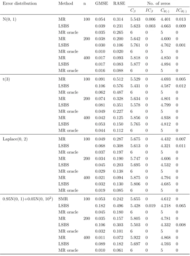
To examine the robustness of the proposed variable selection procedure, we compare the performance of the variable selection procedure based on modal regression (MR) proposed in this paper with that based on the least square B-spline (LSBS) estimator used in Feng and Xue (2013). The simulated results are reported in Table 1. The column labeled “Cβ” in Table 1 gives the average number of zero coefficients
correctly estimated to be zero for parametricβ. Column “ICβ” presents the average number of nonzero
coefficients incorrectly estimated to be zero. While “Cθ(·)” and “ICθ(·)” present the average number of
zero coefficients correctly estimated to be zero and the average number of nonzero coefficients incorrectly estimated to be zero for varying coefficient functionsθ(u), respectively. Furthermore, Table 1 also presents the median of GMSE for the parametric components and the median of RASE for the nonparametric components.
From Table 1, we can make the following observations: (a) For given n, the penalised MR estimate performs better than the penalised LSBS estimator method especially for the non-normal error distribution; (b) For given error distribution, we can see that the variable selection method based on MR and LSBS both become better and better as nincreases. In addition, the performance of the variable selection method based on MR becomes more and more closer to that based on the Oracle procedure asnincreases; (c) For the error distribution is 0.95N(0,1) + 0.05N(0,102), we can see that the superiority of MR becomes more
and more obvious as sample sizenincreases.
5. Conclusions
In this paper, we have proposed a robust variable selection procedure for PVCSIM based on modal regression. The main contributions of the present article can be summarized as follows: (a) our procedures are computationally efficient and theoretically reliable; (b) the variable selection procedure has the oracle property; (c) the estimators of the single-index parametric components, which are of primary interest, are still asymptotically normal.
There are several possible extensions that deserve further study. In our work, we are just concerned with the situation that the covariates are errors free, while it might be interesting to investigate the case where the covariates are subject to measurement errors. Furthermore, Our approach described in this paper can be easily extended to other models, such as partially linear single index model and partially linear additive model. On another direction, it would be interesting to consider the dimensions q go to infinity asn → ∞, the variable selection procedure proposed by this paper will not work any more, for such high-dimensional problems, it is the subject of ongoing research.
Acknowledgements
The authors are deeply grateful to Editor-in-Chief Byeong U. Park, the Associate Editor and two anonymous reviewers for their constructive comments that greatly improved the article. Special thanks go to professor Yao W. (Kansas State University) for his help. The research of Zhu is partially supported by National Natural Science Foundation of China (NNSFC) under Grants 71171075, 71221001 and 71031004. The research of Yu is supported by NNSFC under Grant 11261048.
Appendix: Proofs
For convenience and simplicity, let Cdenote a positive constant that may be different at each appear-ance throughout this paper. For any two sequences {an, bn, n= 1,2, ...}, we write an bn if there are
constants 0 < c1 < c2 <∞ such that c1 ≤ an/bn ≤c2 for all n sufficiently large. Before we prove our
main theorems, we list some regularity conditions that are used in this paper.
C1. The variableU has a bounded support U([a1, b2]) and its density functionfU(·) is positive and has
a continuous second derivative.
C2. The functionθj(u) is the r(r > 2)th continuously differentiable on [0,1], and the functiong(t) has
bounded and continuous derivatives up to orderron [a2, b2].
C3. Let the matrices E(ZZT|U =u) and E(ZXT|U =u) be continuous with respect to u. Furthermore,
for givenu, E(ZZT|U =u) and E(ZXT|U =u) are all positive definite matrix and their eigenvalues are bounded. In addition, we also assume that maxikXik/
√
n=op(1) and maxikZik/
√
n=op(1).
C4. K1K2K.
C5. F(u, t, z) andG(u, t, z) are continuous with respect to (u, t, z). Furthermore, F(u, t, z)<0 for any
h >0. C6. E(φ0h(ε)|U =u, XTβ=t, Z =z) = 0 and E(φ00 h(ε) 2|U =u, XTβ=t, Z =z), E(φ0 h(ε) 3|U =u, XTβ = t, Z=z) and E(φ000h(ε)|U =u, XTβ =t, Z =z) are continuous with respect tot at the pointt0.
C7. Let tj1, ..., tjKj be the interior knots of [aj, bj] for j = 1,2. Moreover, let tj0 = aj, tj,Kj+1 = bj,
hji=cji−cj,i−1and hj = max1≤i≤Kj+1{hji}, Then, there exist a constantC0j satisfy
hj
min1≤i≤Kj+1{hji}
C8. Letbn = maxj,s{|p00λ1j(kγ0jkH)|,|p 00 λ2s(|β (1) 0s|)|:γ0j 6= 0, β (1) 0s 6= 0}, thenbn →0 asn→ ∞.
C9. lim infn→∞lim infβ(1)
s →0+λ −1 2s|p0λ2s(|β
(1)
s |)| > 0 and lim infn→∞lim infkγjkH→0λ1−j1p0λ1j(kγjkH) > 0, wherej=d1+ 1, ..., q,s=d2, ..., p.
These assumptions, while look a bit lengthy, in fact, are quite mild and similar assumptions can be found in Zhao and Xue (2009), Zhao, Zhang, Liu and Lv (2013) and Feng and Xue (2013). The condition
E(φ0h(ε)|u, t, z) = 0 ensures that the proposed estimate is consistent and it is satisfied if the error density is symmetric about zero. More detail can be found in Yao, Lindsay and Li (2012).
Proof of Theorem 1. Letδ=K−r+a
n andv= (v1T, vT2, vT3)T. Define β(1)=β (1)
0 +δv1,η =η0+δv2
andγ=γ0+δv3. Let us first show that, for any given ξ >0, there exists a largeC such that
Pn inf
kvk=CL(e α0+δv)>L(e α0)
o
≥1−ξ. (A.1)
This implies that, with probability at least 1−ξ, there exists a local minimizer in the ball{α0+δv:
kvk ≤C}. Using the Taylor expansion, it follows that
Dn(v)≡nK−1{L(e α0+δv)−L(e α0)} =K−1 n X i=1 n −φh Yi−WiTγ−B2(XiTβ(β (1)))Tη+φ h Yi−WiTγ0−B2(XiTβ(β (1) 0 )) Tη 0 o +nK−1 q X j=1 {pλ1j(kγjkH)−pλ1j(kγ0jkH)}+nK −1 p−1 X s=1 {pλ2s(|β (1) s |)−pλ2s(|β (1) 0s|)} ≥K−1 n X i=1 n −φh Yi−WiTγ−B2(XiTβ(β (1)))Tη+φ h Yi−WiTγ0−B2(XiTβ(β (1) 0 )) Tη 0 o +nK−1 d1 X j=1 {pλ1j(kγjkH)−pλ1j(kγ0jkH)}+nK −1 d2−1 X s=1 {pλ2s(|β (1) s |)−pλ2s(|β (1) 0s|)} = δ K n X i=1 φ0hεi+ZiTR1(Ui) +R2(XiTβ(β (1) 0 )) Qi− δ2 2K n X i=1 φ00hεi+ZiTR1(Ui) +R2(XiTβ(β (1) 0 )) Q2i + δ 3 6K n X i=1 φ000h(ςi)Q3i + n K d2−1 X s=1 {pλ2s(|β (1) s |)−pλ2s(|β (1) 0s|)}+ n K d1 X j=1 {pλ1j(kγjkH)−pλ1j(kγ0jkH)} ≡:I1+I2+I3+I4+I5, (A.2) whereςi is betweenεi+ZiTR1(Ui) +R2(XiTβ(β (1) 0 )) andεi+ZiTR1(Ui) +R2(XiTβ(β (1) 0 ))−δQi,R2(t) = g(t)−B2(t)Tη, R1(u) = (R11(u), ..., R1q(u))T with R1j(u) = θj(u)−B1(u)Tγ0j, j = 1, ..., q and Qi = WiTv3+B2(XiTβ(β (1) 0 )) Tv 2+B02(X T i β(β (1) 0 )) Tη 0vT1J T β(1)Xi+δB 0 2(X T i β(β (1) 0 )) Tη 0v2v1TJ T β(1)Xi. Let us first
considerI1, using Taylor expansion, we obtain that
n X i=1 φ0h εi+ZiTR1(Ui) +R2(XiTβ(β (1) 0 )) Qi= n X i=1 n φ0h(εi) +φ00h(εi) ZiTR1(Ui) +R2(XiTβ(β (1) 0 )) +φ000h(i) ZiTR1(Ui) +R2(XiTβ(β (1) 0 )) 2o Qi,
wherei is betweenεi andεi+ZiTR1(Ui) +R2(XiTβ(β
(1)
0 )). By the condition C1, C2, C7 and Corollary
6.21 in Schumaker (1981), we have kR1j(u)k =O(K−r) and kR2(t)k = O(K−r), and |g0(XiTβ(β(1)))− B20(XT
i β(β(1)))η0| ≤CK−r+1, then we can prove
n X i=1 φ00h(εi)R1(Ui)TZiQi= n X i=1 φ00h(εi)R1(Ui)TZiB2(XiTβ(β (1) 0 )) Tv 2+δB02(X T i β(β (1) 0 )) Tη 0v2vT1J T β(1)Xi + B20(XiTβ(β0(1)))Tη0−g0(XiTβ(β (1) 0 )) v1TJβT(1)Xi+g0(XiTβ(β (1) 0 ))v T 1J T β(1)Xi +WiTv3 =Op(nK−rkvk), (A.3)
using an argument similar to the above, we have Pn
i=1φ
00
h(εi)R2(XiTβ(β
(1)
0 ))Qi = Op(nK−rkvk), then
invoking condition C6 and C7, and some simple calculations, we obtain
n X i=1 φ0hεi+ZiTR1(Ui) +R2(XiTβ(β (1) 0 )) Qi=Op(nK−rkvk).
Thus, we haveI1=Op(nδ2K−1kvk). Similarly, we can prove thatI2=F(U, T, Z, h)Op(nδ2K−1kvk2)
and I3 =Op(nδ3K−1kvk3). Hence, we can choose C large enough such thatI2 dominates bothI1 and
I3 uniformly inkvk =C by noting thatF(U, T, Z, h)<0. Furthermore, invokingpλ(0) = 0, and by the
standard argument of the Taylor expansion, we have
I4≤nK−1 d2−1 X s=1 δp0λ2s(kβ0(1)sk)sgn(β0(1)s)kv1sk+δ2p00λ2s(kβ (1) 0sk)kv1sk2(1 +op(1)) ≤npd2−1K−1δankvk+nK−1δbnkvk2.
Then, it is easy to show thatI4is dominated byI2uniformly inkvk=C. Using an argument similar toI4,
we can prove that I5 is also dominated byI2uniformly inkvk=C. Therefore, by choosing a sufficiently
largeC, A.1 holds. Namely, there exists a local minimizers ˆβ, ˆγ and ˆη such that
kβˆ−β0k=Op(δ), kˆγ−γ0k=Op(δ) and kˆη−η0k=Op(δ), (A.4)
which completes the proof of part (a). Next, we prove part (b).
kθˆj(u)−θ0j(u)k2= Z U {B1(u)Tγˆj−B1(u)Tγ0j+R1j(u)}2du ≤2 Z U {B1(u)Tγˆj−B1(u)Tγ0j}2du+ 2 Z U R1j(u)2du = 2(ˆγj−γ0j)TH(ˆγj−γ0j) + 2 Z U R1j(u)2du, where H = R
UB1(u)B1(u)Tdu. Then, invoking kHk = O(1) and kˆγ−γ0k = Op(δ), after a simple
calculation yields
Furthermore, it is easy to obtain that
Z
U
R1j(u)2du=Op(K−2r). (A.6)
Therefore, combing A.5 and A.6, the proof of part (b) is completed.
Proof of Theorem 2. We only show part (a) as an illustration and part (b) is similar. Fromλmax→0,
it is easy to show thatan = 0 for largen. Then by Theorem 1, it is sufficient to show that, for anyβ
(1)
s
which satisfieskβs(1)−β0(1)sk=Op(K−1) for s= 1, ..., d2−1, and some given smallζ=CK−1, asn→ ∞,
with probability approaching one, we have
∂eL(α) ∂βs(1) >0, 0< βs(1)< ζ, s= 1, ..., d2−1, ∂eL(α) ∂βs(1) <0, −ζ < βs(1)<0, s= 1, ..., d2−1. Note that n∂eL(α) ∂βs(1) = n X i=1 φ0hYi−WiTγ−B2(XiTβ(β (1)))TηB0 2(X T i β(β (1)))TηΓT β(1)s Xi+np0λ2s(|β (1) s |)sgn(β (1) s ) = n X i=1 φ0hεi+ZiTR1(Ui) +R2(XiTβ(β (1) 0 )) + Ωi B20(XiTβ(β(1)))TηΓT βs(1) Xi+np0λ2s(|β (1) s |)sgn(β (1) s ) = n X i=1 ( φ0hεi+ZiTR1(Ui) +R2(XiTβ(β (1) 0 )) +φ00hεi+ZiTR1(Ui) +R2(XiTβ(β (1) 0 )) Ωi +φ000h(ωi)Ω2i ) [g0(XiTβ(β(1)))−B20(XiTβ(β(1)))Tη0]−g0(XiTβ(β (1))) +B0 2(X T i β(β (1) 0 )) T(η 0−η) + [B20(XiTβ(β0(1)))−B20(XiTβ(β(1)))]TηπT βs(1) Xi+np0λ2s(|β (1) s |)sgn(β (1) s ), (A.7) where πβ(1) s = (−β (1) s / p
1− kβ(1)k2,0, ...,0,1,0, ...,0)T is ap×1 vector with the (s+ 1)th component 1, ωi is betweenεi+ZiTR1(Ui) +R2(XiTβ(β (1) 0 )) andεi+ZiTR1(Ui) +R2(XiTβ(β (1) 0 )) + Ωi, and Ωi=WiT(γ0−γ) +B2(XiTβ(β (1) 0 ))(η0−η) + [B2(XiTβ(β (1) 0 ))−B2(XiTβ(β (1)))]Tη.
Using an argument similar to A.3, and invoking A.4, it is easy to show that
n∂eL(α) ∂βs(1) =nλ2s λ−2s1p0λ2s(|β (1) s |)sgn(βs(1)) +Op(λ−2s1K −r) ,
since by the condition C9, limn→∞lim infβ(1)
s →0λ −1 2sp0λ2s(|β
(1)
s |)>0 andλ2sKr≥λminKr→ ∞, thus, the
sign of A.7 is completely determined by that ofβs(1). This completes the proof of part (a).
to 1,L(e α) attains the minimal vale at (ˆγAT,0)T, ( ˆβ (1)T A ,0)T and ˆη. Define ˆαA= (ˆγAT,0)T,η,ˆ ( ˆβ (1)T A ,0)T T , ∂L( ˆeαA) ∂βA(1) =−1 n n X i=1 φ0hYi−WiTAγˆA−ˆg(XiTAβ( ˆβ (1) A )) ˆ g0(XT iAβ( ˆβ (1) A ))J T ˆ β(1)A XiA +p0λ2(|β (1) A |)∗sgn(β (1) A ) = 0, ∂L( ˆeαA) ∂γA =−1 n n X i=1 φ0hYi−WiTAγˆA−ˆg(XiTAβ( ˆβ (1) A )) WiA+ ∆ = 0,
where “∗” denotes the Hadamard product and the sth component ofp0λ
2(|β (1) A |) is p0λ2s(|β (1) sA|) for s = 1, ..., d2−1, and ∆ = p0λ 11(kˆγ1kH) ˆ γT 1H kˆγ1kH , ..., p0λ 1d1(kˆγd1kH) ˆ γTd 1H kˆγd1kH !T .
Using the Taylor expansion top0λ
2s(| ˆ βs(1)|), we get that p0λ2s(|βˆ(1)s |) =p0λ2s(|βˆ0(1)s|) +{p00λ2s(|βˆ0(1)s|) +op(1)}( ˆβs(1)−β (1) 0s). By condition C8, we have p00λ 2s(| ˆ
β0(1)s|) = op(1), and note that p0λ2s(| ˆ
β(1)0s|) = 0 as λmax → 0. Then,
from Theorems 1∼2, we have p0λ
2s(| ˆ βs(1)|)sgn( ˆβ (1) s ) = op( ˆβ (1) s −β (1)
0s). Similarly, we can prove that p0
λ1j(kˆγjkH)(Hγˆj/kˆγjkH) = op(ˆγj−γ0j). Thus, invoking Lemma A.1 in Feng and Xue (2013), after a simple calculation yields
0 =−1 n n X i=1 φ0h εi+ZiTAR1A(Ui) +g(XiTAβ(β (1) 0A))−ˆg(X T iAβ( ˆβ (1) A ))−W T iA(ˆγA−γ0A) g0(XiTAβ(β(1)0A))JT β0(1)AXiA+op( ˆβ (1) A −β (1) 0A) +op(n−1/2), (A.8) 0 =−1 n n X i=1 φ0hεi+ZiTAR1A(Ui) +g(XiTAβ(β (1) 0A))−ˆg(X T iAβ( ˆβ (1) A ))−W T iA(ˆγA−γ0A) WiA+op(ˆγA−γ0A). (A.9)
To make our mathematical formula short, let Πi = ZiTAR1A(Ui) +g(XiTAβ(β
(1) 0A))−gˆ(XiTAβ( ˆβ (1) A ))− WT iA(ˆγA−γ0A) and GiA=g0(XiTAβ(β (1) 0A))JβT(1) 0A
XiA. Applying the Taylor expansion to A.8 and A.9, we obtain that 0 =− 1 n n X i=1 n φ0h(εi) +φ00h(εi)Πi+ 1 2φ 000 h(ε∗i)Π 2 i o GiA+op( ˆβ (1) A −β (1) 0A) +op(n−1/2), (A.10) 0 =− 1 n n X i=1 n φ0h(εi) +φ00h(εi)Πi+ 1 2φ 000 h(ε∗∗i )Π 2 i o WiA+op(ˆγA−γ0A), (A.11)
where bothε∗i andε∗∗i lie betweenεandε+ Πi.
Define Λn = n−1P n i=1φ 00 h(εi)WiAWiTA, Ξn = n−1P n i=1φ 00 h(εi)WiA[g(XiTAβ(β (1) 0A))−ˆg(XiTAβ( ˆβ (1) A ))], Φn=n−1P n i=1WiA[φ0h(εi) +φ00h(εi)ZiTAR1A(Ui)] and Ψn=n−1P n
conditions C5∼C6, and Theorem 1∼2, we have ˆ γA−γ0A= (Λn+op(1))−1(Φn+ Ξn). (A.12) Note that g(XiTAβ(β (1) 0A))−ˆg(X T iAβ( ˆβ (1) A )) =g(X T iAβ(β (1) 0A))−g(X T iAβ( ˆβ (1) A )) +g(X T iAβ( ˆβ (1) A ))−ˆg(X T iAβ( ˆβ (1) A )) =GTiA(β(1)0A−βˆA(1)) +op(β (1) 0A−βˆ (1) A ) +Op(K−r). (A.13)
Substituting A.12 into A.10, and a simple calculation yields
n n−1 n X i=1 φ00h(εi)GiAGeTiA+op(1) o√ n( ˆβ(1)A −β0(1)A) = √1 n n X i=1 n GiAφ0h(εi) +φ00h(εi)GiAZiTAR1A(Ui) +φ00h(εi)GiAWiTA(Λn+op(1))−1Φn o . (A.14) Note thatn−1Pn i=1Ψ T nΛ− 1 n WiAGeiA= 0 withGeiA=GTiA−WiTAΛ−n1Ψn, andn−1P n i=1Ψ T nΛ− 1 n WiA(φ0h(εi)+ φ00h(εi)ZiTAR1A(Ui)−φ00h(εi)WiTAΛ−n1Φn) = 0. Therefore, A.14 can be rewritten as follows
n n−1 n X i=1 φ00h(εi)GeiAGeTiA+op(1) o√ n( ˆβ(1)A −β0(1)A) = √1 n n X i=1 n e GiAφ0h(εi) +φ00h(εi)GeiAZiTAR1A(Ui) +φ00h(εi)GeiAWiTAΛ−n1Φn o +op(1). ≡:L1+L2+L3+op(1). (A.15)
It is easy to show thatn−1Pn
i=1φ
00
h(εi)GeiAWiTA= 0 and by the definition ofR1A(Ui), we can prove that
1 √ n Pn i=1φ 00
h(εi)GeiAZiTAR1A(Ui) =op(1). Now let us deal with the first termL1, By directly calculating its
expectation and variance, we have E(L1) = 0 and cov(L1) = E(G(U, T, Z, h)GeiAGeTiA), this follows easily
by checking Linderbergs condition. In addition, by the law of large numbers, we have
n−1 n X i=1 φ00h(εi)GeiAGeTiA p −→Σ1, (A.16)
and from the definition ofJβ(1) 0A of Eq.(2.4), it follows ( ˆβA−β0A) = Jβ(1) 0A ( ˆβA(1)−β(1)0A) +Op(n−1). Thus, we have √ n( ˆβA−β0A) =Jβ(1) 0A Σ−11√1 n n X i=1 e GiAφ0h(εi) +op(1). Therefore, we have √ n( ˆβA−β0A) D −→N(0, Jβ(1) 0A Σ−11ΣΣ−11JT β0(1)A), (A.17)
References
[1] Eddy, W. F. (1980). Optimum kernel estimators of the mode. The Annals of Statistics, 870-882. [2] Fan, J., & Li, R. (2001). Variable selection via nonconcave penalized likelihood and its oracle
prop-erties.Journal of the American Statistical Association, 96(456), 1348-1360.
[3] Feng, S., & Xue, L. (2013). Variable selection for partially varying coefficient single-index model. Journal of Applied Statistics, 2637-2652.
[4] Frank, L. E., & Friedman, J. H. (1993). A statistical view of some chemometrics regression tools. Technometrics, 35(2), 109-135.
[5] Huang, Z. (2011). Empirical likelihood-based inference in varying-coefficient single-index models. Journal of the Korean Statistical Society, 40(2), 205-215.
[6] Huang, Z., Lin, B., Feng, F., & Pang, Z. (2013). Efficient penalized estimating method in the partially varying-coefficient single-index model.Journal of Multivariate Analysis, 114, 189-200.
[7] Huang, Z., & Zhang R. (2010). Empirical likelihood for the varying-coefficient single-index model. The Canadian Journal of Statistics, 38, 434-452.
[8] Li, J., Ray, S., & Lindsay, B. G. (2007). A Nonparametric Statistical Approach to Clustering via Mode Identification.Journal of Machine Learning Research, 8(8), 1687-1723.
[9] Liu, J., Zhang, R., Zhao, W., & Lv, Y. (2013). A robust and efficient estimation method for single index models.Journal of Multivariate Analysis, 122, 226-238.
[10] Li, R., & Liang, H. (2008). Variable selection in semiparametric regression modeling. Annals of Statistics, 36(1), 261-286.
[11] Romano, J. P. (1988). On weak convergence and optimality of kernel density estimates of the mode. Annals of Statistics, 16, 629-647.
[12] Schumaker, L. L. (1981).Spline functions: basic theory. New York: Wiley.
[13] Tibshirani, R. (1996). Regression shrinkage and selection via the lasso.Journal of the Royal Statistical Society. Series B, 267-288.
[14] Wang, J. L., Xue, L., Zhu, L., & Chong, Y. S. (2010). Estimation for a partial-linear single-index model. The Annals of statistics, 38(1), 246-274.
[15] Wang, Q., & Wu, R. (2013). Shrinkage estimation of partially linear single-index models. Statistics and Probability Letters. 83(10), 2324-2331.
[16] Wang, Q., & Xue, L. (2011). Statistical inference in partially-varying-coefficient single-index model. Journal of Multivariate Analysis, 102(1), 1-19.
[17] Wong, H., Ip, W. C.,& Zhang, R. (2008). Varying-coefficient single-index model. Computational s-tatistics and data analysis, 52(3), 1458-1476.
[18] Wu, T. Z., Yu, K., & Yu, Y. (2010). Single-index quantile regression.Journal of Multivariate Analysis, 101(7), 1607-1621.
[19] Yao, W., Lindsay, B. G., & Li, R. (2012). Local modal regression.Journal of nonparametric statistics, 24(3), 647-663.
[20] Yu, Y., & Ruppert, D. (2002). Penalized spline estimation for partially linear single-index models. Journal of the American Statistical Association, 97(460), 1042-1054.
[21] Zhang, R., Zhao, W., & Liu, J. (2013). Robust estimation and variable selection for semiparamet-ric partially linear varying coefficient model based on modal regression. Journal of Nonparametric Statistics, 25(2), 523-544.
[22] Zhao, P., & Xue, L. (2009). Variable selection for semiparametric varying coefficient partially linear models.Statistics and Probability Letters, 79(20), 2148-2157.
[23] Zhao, W., Zhang, R., Liu, J., & Lv, Y. (2014). Robust and efficient variable selection for semipara-metric partially linear varying coefficient model based on modal regression.Annals of the Institute of Statistical Mathematics, 66(1), 165-191.
[24] Zou, H. (2006). The adaptive LASSO and its oracle properties.Journal of the American Statistical Association, 101, 1418-1429.
Table 1:Simulation results
Error distribution Method n GMSE RASE No. of zeros
Cβ ICβ Cθ(·) ICθ(·) N(0, 1) MR 100 0.054 0.314 5.543 0.006 4.401 0.013 LSBS 0.039 0.231 5.623 0.003 4.663 0.009 MR oracle 0.035 0.265 6 0 5 0 MR 200 0.038 0.200 5.642 0 4.600 0 LSBS 0.030 0.106 5.761 0 4.762 0.001 MR oracle 0.010 0.020 6 0 5 0 MR 400 0.017 0.093 5.818 0 4.850 0 LSBS 0.017 0.083 5.877 0 4.894 0 MR oracle 0.016 0.088 6 0 5 0 t(3) MR 100 0.091 0.512 5.529 0 4.693 0.005 LSBS 0.106 0.576 5.431 0 4.587 0.012 MR oracle 0.062 0.487 6 0 5 0 MR 200 0.074 0.328 5.634 0 4.801 0 LSBS 0.081 0.351 5.578 0 4.799 0 MR oracle 0.049 0.227 6 0 5 0 MR 400 0.042 0.125 5.856 0 4.938 0 LSBS 0.053 0.150 5.765 0 4.812 0 MR oracle 0.044 0.112 6 0 5 0 Laplace(0, 2) MR 100 0.049 0.287 5.675 0 4.432 0.007 LSBS 0.068 0.308 5.613 0 4.321 0.011 MR oracle 0.037 0.197 6 0 5 0 MR 200 0.034 0.190 5.747 0 4.606 0 LSBS 0.045 0.203 5.695 0 4.532 0 MR oracle 0.029 0.138 6 0 5 0 MR 400 0.021 0.094 5.875 0 4.794 0 LSBS 0.032 0.130 5.806 0 4.685 0 MR oracle 0.019 0.085 6 0 5 0 0.95N(0, 1)+0.05N(0, 102) SMR 100 0.053 0.242 5.655 0 4.612 0 LSBS 0.182 0.496 5.428 0.019 4.218 0.065 MR oracle 0.045 0.180 6 0 5 0 MR 200 0.035 0.157 5.805 0 4.781 0 LSBS 0.106 0.303 5.503 0 4.332 0.008 MR oracle 0.032 0.101 6 0 5 0 MR 400 0.011 0.072 5.922 0 4.868 0 LSBS 0.089 0.182 5.697 0 4.593 0 MR oracle 0.010 0.061 6 0 5 0