SWAN vs. DG-WAVE: A Comparison of Numerical Wave Prediction Models

(1)

SWAN vs. DG–WAVE

A Comparison of Numerical Wave Prediction Models

A Thesis

Presented in Partial Fulfillment of the Requirements for

Graduating with Research Distinction in the

Undergraduate School of The Ohio State University

By

Rachel A. Sebian,

Undergraduate Program in Civil Engineering

The Ohio State University

2013

Examination Committee:

Ethan J. Kubatko, Advisor

(2)

c

Copyright by

Rachel A. Sebian 2013

(3)

Acknowledgement

I would like to thank my research advisor, Professor Ethan Kubatko, for giving me the opportunity to complete this research project, as well as all of my colleagues in the C.H.I.L for supporting and assisting me during this process.

I would also like to thank my loving parents and grandfather who support me in everything I do and without whom I would not be where I am today.

(4)

LIST OF TABLES

Table Page

4.1 Computational times in minutes for the months of May through

(7)

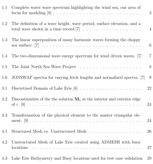
LIST OF FIGURES

Figure Page

1.1 Complete water wave spectrum highlighting the wind sea, our area of

focus for modeling [8] . . . 3

1.2 The definition of a wave height, wave period, surface elevation, and a

total wave shown in a time record.[7] . . . 4

1.3 The linear superposition of many harmonic waves forming the choppy

sea surface. [7] . . . 6

1.4 The two-dimensional wave energy spectrum for wind driven waves. [7] 7

1.5 The Joint North Sea Wave Project . . . 8

1.6 JONSWAP spectra for varying fetch lengths and normalized spectra. [7] 9

3.1 Discretized Domain of Lake Erie [8] . . . 22

3.2 Discontinuities of the the solutionMh at the interior and exterior edge

of i. [9] . . . 24

3.3 Transformation of the physical element to the master triangular

ele-ment. [9] . . . 24

4.1 Structured Mesh vs. Unstructured Mesh . . . 26

4.2 Unstructured Mesh of Lake Erie created using ADMESH with buoy

locations . . . 27

(8)

4.4 Significant Wave Heights Time Series Comparison for June 2011 at

Buoys 45005, 45132, and 45142 . . . 31

4.5 Significant Wave Heights Time Series Comparison for August 2011 at

Buoys 45005, 45132, and 45142 . . . 32

4.6 Significant Wave Heights Time Series Comparison for October 2011 at

Buoys 45005, 45132, and 45142 . . . 33

4.7 Computational time comparisons from simulations run with SWAN vs

(9)

CHAPTER 1

INTRODUCTION

In the sense of real world application, the largest motivation for developing wind-driven wave models such as SWAN and DG–WAVE is to predict the behavior of the ocean surface throughout different weather events over time. The behavior of the ocean surface is important for many reasons, some relevant from an engineering standpoint and others relevant from a personal standpoint. An individual might want to know future ocean wave behavior for safety purposes related to surfing or boating, while the engineer seeks to model the behavior of the water body in an effort to relate it to weather safety, shore infrastructure or other fluid related design.

Established wave models are frequently used by government organizations such as NOAA (National Oceanic and Atmospheric Administration), the U.S. Army Corps of Engineers, FEMA (Federal Emergency Management Agency), and the Louisiana State University Hurricane Center. These organizations often utilize wave models as a component of comprehensive ocean and lake modeling to simulate past or future events with extreme weather circumstances in order to better understand issues such as structural damage, flooding, pollution transport, or erosion. Examples of these situations are disasters such as hurricanes, tsunamis, or oil spills; all of which benefit from both forecast and hind cast simulations to increase scientific knowledge about

(10)

the event. In order to accurately simulate these events, wave models are coupled with other models that add additional detail to the simulation; for example, in practice SWAN is often utilized coupled with the ADvanced CIRCulation model (ADCIRC).

1.1

Motivations for Modeling Wind-Driven Waves

The dynamics of the surface of large, open bodies of water such as lakes and oceans is extremely complex. From a mathematical standpoint, the approach taken is determined largely by the constraints of the problem at hand. For example, the study of a shallow water body located directly on the coast with a domain on the order of meters would require a very different numerical approach than the study of a water body in the middle of the Atlantic Ocean with a domain on the order of kilometers. There are a variety of scientific motivations for creating a model to describe wind-driven waves, however, in the case of our applications we seek to resolve the solution over a relatively large domain typically on the order of hundreds of wave periods. For this reason our motivation need not be directed toward determining an exact solution over the entire domain, but rather focused on finding an approximate solution over the whole domain which gives an effective characterization of the sea state. There are several reasons an exact solution is unnecessary for this type of scale, the most important of which being that the problem is simply computationally unrealistic. Unique situations could arise in which such detail is necessary, however the problem we address in this study is not one of them nor are most typical cases.

(11)

1.2

Background

In large bodies of water, waves of many different types propagate with a wide range of periods and frequencies due to external forces both natural and man-made. The waves we are interested in modeling are surface gravity waves, short waves with periods on the order of seconds and wavelengths on the order of meters which develop after force is applied from local winds to the water surface. In the spectrum of all water waves this is characterized as the wind sea, as shown in Figure 1.1.

seconds minutes hours days months years

<1 sec TIDES CAPILLARY SWELL TSUNAMIS PLANETARY Wind Large-scale

disturbances (Earth & Moon)Gravitational shape & rotationEarth’s Force:

Period:

WIND SEA

Type: Generating

Figure 1.1: Complete water wave spectrum highlighting the wind sea, our area of focus for modeling [8]

Models simulating surface gravity waves produce a variety of output values, most often values which represent the average of a sea surface attribute rather than an exact measurement. The value of most relevance for typical users and for this study is significant wave height, which is typically defined as the mean of the highest one-third of waves in the wave record [7]. To fully understand this concept, let us go into some detail on the definition of waves and wave height. Wave height is commonly confused with surface elevation; surface elevation being defined as the instantaneous eleveation of the sea surface at any one moment relevant to a reference zero level within a time record. In the same time record, a wave would be defined as the profile

(12)

of the surface elevation between two successive downward or two successive upward zero-crossing on the elevation. This concept as well as wave height and wave period are illustrated in Figure 1.2.

Figure 1.2: The definition of a wave height, wave period, surface elevation, and a total wave shown in a time record.[7]

One wave only has one wave height, thus in a time record with Nwaves the mean

wave height H at a given point is defined as:

H= 1 N N X i=1 Hi (1.1)

where i is the sequence number of the wave in the record. Although the mean wave

(13)

well correlated with visually estimated wave height. Thus another wave height is introduced, the aforementioned significant wave height, defined mathematically as:

H1/3 = 1 N/3 N/3 X j=1 Hj (1.2)

wherej is not the sequence number but the rank number based on wave height (j = 1

is the highest wave, j = 2 is the second-highest wave, ect.).

Today there are several well-established wave prediction models available which are proficient in providing an accurate simulation of the sea state, namely SWAN, the WAM model, and WAVEWATCH III. These well-known models are utilized for the majority of wave-prediction modeling performed by federal and state organizations like the National Weather Service as well as private institutions. In particular, the SWAN model is widely used by a number of agencies and institutions, and will be one of the models considered in this study. The other model considered will be the DG– WAVE model, recently developed in the Computational Hydrodynamics Informatics Laboratory at the Ohio State University [8].

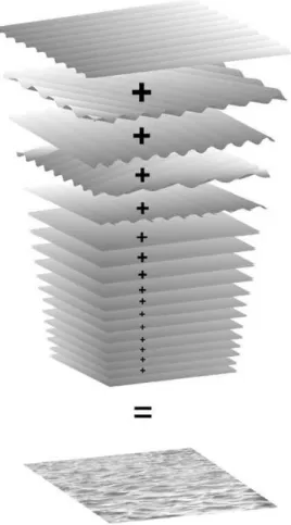
Since the origins of wind-driven wave modeling in the 1950s and 1960s, two ap-proaches have been developed for the purpose of characterizing short waves with pe-riods on the order of seconds: the phase-averaged approach and the phase-resolving approach. The phase-averaged approach regards the sea state as a stochastic process that can be depicted as a spectral decomposition, where wave energy is attributed to the superposition of many harmonic waves with distinct directions and periods, as shown in Figure 1.3.

(14)

Figure 1.3: The linear superposition of many harmonic waves forming the choppy sea surface. [7]

The phase-averaged approach seeks to characterize all possible sea states that could arise while conditions of the actual observation were occurring, i.e., describ-ing the average sea state durdescrib-ing that time period. Conversely, the phase-resolvdescrib-ing approach solves explicitly for sea state conditions in time thus requiring much more computational power if applied to anything other than a very small domain. For these reasons, the phase-averaged approach is considerably more effective when the application takes place on a large domain (such as our Lake Erie application).

(15)

Within the group of models which employ the phase-averaged approach are spec-tral models, so-called because they utilize the variance density spectrum to relate wave energy to the variance of the ocean’s free surface. Spectral models make the assumption that the wave field develops gradually in time and space over the scale of a single wavelength. In such a model, energy is split into spectral components with discrete frequencies traveling in different directions bands. The wave energy spectrum for wind-driven waves characterizes the distribution of the sea surface over directions and frequencies, as shown in Figure 1.4. SWAN is a spectral model in that it solves for wave energy directly.

Figure 1.4: The two-dimensional wave energy spectrum for wind driven waves. [7]

DG–WAVE is unique from other spectral models in that it is based on a parametric approach. Parametric models simplify the relationship between model parameters by making assumptions about spectral shape. In doing so, the model avoids solving over

(16)

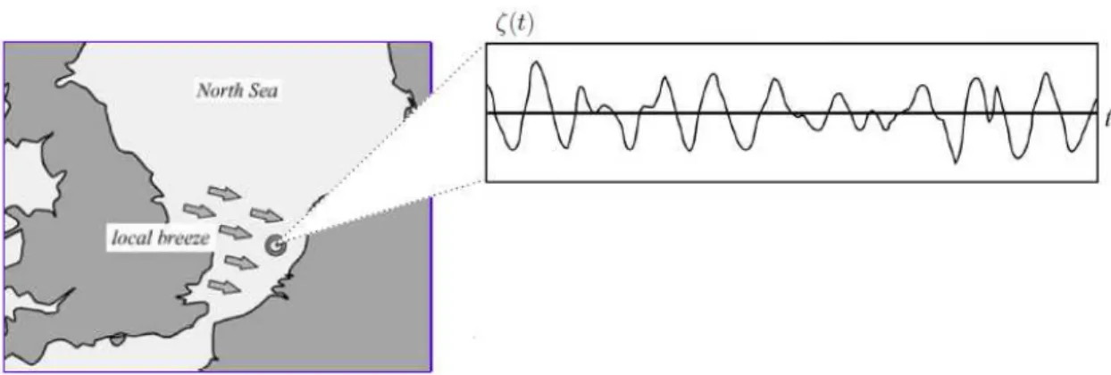
many discrete frequencies and directional bins like many existing spectral models, which can often be computationally inefficient. In the case of DG–WAVE, wave energy is parameterized using the JONSWAP design spectrum. The Joint North Sea WAve Project (JONSWAP) was an extensive wave experiment conducted in 1968 which measured wave spectra for various wind conditions in the North Sea region, as illustrated in Figure 1.5.

Figure 1.5: The Joint North Sea Wave Project

The data was used to compile energy spectra for differing fetch lengths, where the term ’fetch’ refers to the length of water over which the wind has blown to invigorate the waves. Thus, the design spectrum, as shown in Figure 1.6, is a fetch-limited spectra defining the distribution of energy with frequency in the ocean.

(17)

Figure 1.6: JONSWAP spectra for varying fetch lengths and normalized spectra. [7]

1.3

Objectives

When applying a numerical model computational time is one of the most impor-tant elements to take into consideration. All numerical wave prediction models arrive

(18)

at a solution by solving a set of governing equations which describe the dynamics occurring within the fluid body. The techniques used to reach these solutions differ among models. The SWAN model is a spectral wave model, using the two-dimensional

variance density spectrumE(f, θ) to solve the action balance equation in five

dimen-sions (t, x, y, σ, θ) (The mathematical basis of the SWAN model will be discussed

further in Chapter 2). SWAN then solves its governing equation, the action balance equation, iteratively at discrete frequency and direction bins until some break-off cri-teria are met. Though this method performs well in application, it is computationally expensive and thus inefficient. This noted inefficiency (which propagates in all spec-tral wave models, not just SWAN) leads to an interest in exploring the potential of a simpler wave model, the GLERL–Donelan wave model. This model utilizes differ-ent model equations to simplify the problem and reduce the number of dimensions as well as avoid performing iterative calculations (The mathematical basis of the Donelan model will be discussed further in Chapter 3). The model was also created with the intention of easy application through a computer system. A discontinu-ous Galerkin method was selected as the approach to implementation and was then developed into a computer interface for the model, a Discontinious Galerkin-based Wave Prediction Model (DG–WAVE). The study presented herein was motivated by the aforementioned work with DG–WAVE and a desire to further investigate a fair comparison of the model’s accuracy as well as computational efficiency with existing wave models (namely SWAN).

(19)

1.4

Thesis Organization

The thesis presented herein is organized as follows. Chapter 2 presents an intro-duction to the Simulating WAves Nearshore (SWAN) Model, it’s derivation from the action balance equation and an overview of how it is operated. Chapter 3 presents an introduction to a Discontinuous Galerkin-based Wave Prediction model (DG–WAVE) and its basis in the Donelan wave model. Chapter 4 presents the test problem rele-vant to this study, going on to provide results and discuss their significance. Chapter 5 ends with a conclusion and discussion of future work.

(20)

CHAPTER 2

A BRIEF OVERVIEW OF THE SWAN MODEL

This chapter provides an overview of the SWAN model including the model for-mulation as well as a brief discussion of input commands and their significance.

2.1

Relevant Model Background

SWAN is a wave model widely used by engineers and scientists for wave research and consultancy practice in industry. The model is third-generation, meaning it explicitly represents all relevant physics for the development of the sea state in two dimensions. Further detail on first, second, and third generation wave models can be found in [6]. The SWAN computer model is open source, freely accessible for use and available for download on line along with a variety of supporting resources. Using available input data (wind, current, water velocity), SWAN computes random, short-crested wind-generated waves in coastal regions and inland waters. There are a variety of available outputs including average wave direction, dissipation, and significant wave height. SWAN can be applied on any scale relevant for wind generated surface gravity waves, however it is specifically designed for coastal applications.

This chapter introduces some of the basic formulations and numerical techniques used to develop SWAN, most importantly its basis in the action balance equation.

(21)

For further background information, a comprehensive and detailed description of the SWAN Wave Model and its development can be found in [7]. The development and upkeep of the model is supported by the Office of Naval Research and Rijkswaterstaat (Ministry of Transport, Public Works and Water Management, The Netherlands). In practice, SWAN is often coupled with the coastal circulation model ADCIRC (Advanced Circulation Model), referred to as SWAN-ADCIRC.

When designing for operational use, the computational time of a numerical wave model is a very important consideration. The computing time of the model is largely impacted by the numerical schemes applied, particularly when representing the prop-agation of waves through geographic space. In the case of this model, an implicit finite-difference scheme is selected because it is both simple and robust as well as considered economical for large-scale applications. The model formulations in SWAN which represent wave invigoration by wind, quadruplet wave-wave interactions, white-capping, and bottom friction are consistent with those of the WAM model. SWAN supplements these formulations with representations of depth-induced breaking and triad wave-wave interactions. For the purpose of this study, the only process of rele-vance is generation by wind. [7]

2.1.1

The Action Balance Equation

Similar wave prediction models are typically based in the energy balance equation

in terms of absolute radian frequency ω. However, the SWAN model is based on the

spectral action balance equation in terms of relative radian frequencyσbecause unlike

(22)

of the action balance equation in Cartesian coordinates (applicable for small-scale computations) is given as ∂N(σ, θ;x, y, t) ∂t + ∂cg,xN(σ, θ;x, y, t) ∂x + ∂cg,yN(σ, θ;x, y, t) ∂y + ∂cθN(σ, θ;x, y, t) ∂θ + ∂cσN(σ, θ;x, y, t) ∂σ = S(σ, θ;x, y, t) σ , (2.1)

whereσ is relative radian frequency,θ is propogation direction (the direction normal

to the wave crest of each spectral component), t is time, cg is group velocity and

geographic space is described by x and y in Cartesian co-ordinates. N(σ, θ) is the

action density spectrum and S(σ, θ) is the source term in terms of energy density,

representing the effects of wave generation, non-linear wave-wave interactions, and dissipation. Equation 2.1 simplifies to the aforementioned energy balance equation when an ambient current is absent:

∂E(ω, θ;x, y, t) ∂t + ∂cg,xE(ω, θ;x, y, t) ∂x + ∂cg,yE(ω, θ;x, y, t) ∂y + ∂cθE(ω, θ;x, y, t) ∂θ =S(ω, θ;x, y, t), (2.2)

where ω is absolute radian frequency, E(ω, θ) is the energy density spectrum and

S(ω, θ) is the source term as described above. For large-scale computations such as

applications with oceanic waters or the Great Lakes, SWAN offers the spectral action balance equation formulated in terms of spherical coordinates. The spherical

formu-lation uses longitude λ and latitude ϕ rather than Cartesian coordinates and is the

formulation utilized in the tests performed in this study. SWAN is comprehensive in that it is capable of performing computations ranging from large-scale, time depen-dent cases with the two-dimensional action balance equation in spherical coordinates

(23)

to small-scale, stationary cases with the one-dimensional energy balance equation in Cartesian coordinates.

2.1.2

Generation by Wind

While SWAN is capable of taking multiple unique source terms into consideration, wind is the most important forcing term driving the model as well as the only term relevant for the purpose of our application. The wind speed fed into the model driving

the propagation of waves is the wind speed at 10 meter elevation,U10, however when

used in the computations it is converted to the friction velocity u∗ by the relation

u2

∗ = CDU

2

10 in which CD is the wind-drag coefficient. CD is determined by a set of

equations expressing wind drag as a function of wind speed. Wave generation by wind is described in the model using the Miles feedback mechanism, supplemented with an initial wave growth term calculated from the Cavaleri and Malanotte-Rizzoli [7] empirical expression using a cut-off to avoid growth at unrealistically low frequencies. With the calculation of other constants given as a function of wind speed, an equation

for total surface stressτwavecan then be solved iteratively. There are three alternative

up-wind schemes available within SWAN for propagation in geographic space, we utilize the BSBT (backward space backward time) scheme which is optimal for non-stationary cases. Change in time is dealt with through a simple backward finite-difference scheme and the subsequent discretization of Equation 2.2 for the BSBT scheme is again solved iteratively, allowing us to arrive at the source term in terms of energy density. For a highly detailed reference on these formulations and numerical methods please see Chapter 9 of [7].

(24)

2.2

Commands and Parameterization

SWAN user support provided by Delft University of Technology is distributed in four separate documents. These documents are the SWAN User Manual, Imple-mentation Manual, Programming rules and Scientific/Technical docuImple-mentation. The SWAN User Manual provides the majority of relevant information for a new user. When executing the SWAN model for the domain of Lake Erie, many months were simulated consistently using the same input commands and parameters. Spherical coordinates were utilized because of a larger domain. The solution was computed using an unstructured computational mesh, further described in Chapter 4. For

com-putation, SWAN utilizes two meshes: one describing the physical (x, y) space of the

domain (the unstructured mesh) and another describing spectral space in terms of

(ω, θ) and (σ, θ). The spectral mesh is parameterized by the frequency, lowest discrete

frequency, and number of bins which were selected after performing several sensitivity analyses to optimize their values. The physics is run in third-generation linear growth mode with a BSBT propagation scheme. The numerics are set at default values for unstructured meshes and maximum number of iterations before cut off is twenty. Sig-nificant wave height is output for three unique points at 10 minute intervals over the course of each month in the form of a DAT file.

(25)

CHAPTER 3

A BRIEF OVERVIEW OF DG–WAVE

This chapter provides an overview of the model background, formulation and implementation as well as a description of model parameters and execution.

3.1

Background

The model presented in this chapter was developed based on the parametric wave equations originally formulated by Mark A. Donelan for Canada’s National Water Resources Institute in 1977 [5]. When developing the model formulas, Donelan made use of the widely accepted Joint North Sea Wave Project (JONSWAP) empirical spectra to simplify the relationship between model parameters and avoid the com-plex process of solving for the evolution of the wave spectra necessary in other well established spectral models. Within the formulas, wind stress is the only forcing source term, meaning the sole input is overlake wind at each point. This approach is contrary to that taken by spectral models which account for each physical pro-cess individually with multiple unique sources terms. David Schwab, et al, was the first to publish results on the application of Donelan’s model equations using a finite difference scheme [2]. Schwab was also the first to make some modifications to the ex-isting model in the interest of conforming to the Great Lakes Environmental Research

(26)

Lab two-dimensional lake circulation modeling system, leading to the what is com-monly known today as the GLERL–Donelan wave model [3]. The results published by Schwab included two parts, verification testing the models consistency against em-pirical formulas for significant wave height in the case of fetch-limited waves (waves limited in height due to size of the wind-wave generation area), and validation of the model tested against data from two locations in Lake Erie for September and October of 1981. Lake Erie is an appropriate choice for this application due to its unique dy-namics, relatively shallow depth and exposure to strong winds such that wind forcing is the dominant mechanism affecting the wave propagation on the lake. After the formulation of DG–WAVE, Schwab’s approach was emulated by both verifying the model numerically using empirical equations and validating the model by application to Lake Erie. [8]

The output we are most interested in from this model is significant wave height, as described in Chapter 1. In order to solve Donelan’s equations, we utilize a discontinu-ous Galerkin finite element method applied on an unstructured mesh. Solving for wave

momentum, we can then find significant wave height using the relation Hs = 4×σ,

where σ is the square root of the variance of the sea surface elevation. The research

described here was motivated by an interest in testing the application of the model when employing the DG framework rather than an interest in validating Donelan’s model equations. Through previous research and publications it has been concluded that the main source of error in applying the model to a real forecast situation will be the quality of the wind data rather than model inadequacies [3].

(27)

3.2

The Numerical Model

As with all numerical models, DG–WAVE is able to describe the sea state of a given domain by finding a solution to some governing equation(s). The governing equation of DG–WAVE’s numerical model is a two-dimensional momentum balance equation based on linear wave theory, notably simpler than the action balance equation solved in the SWAN model. The basic model equations relate the time rate of change of total wave momentum (per unit surface area, per unit specific weight) to the divergence of wave momentum flux with momentum input due to wind stress as follows:

∂M

∂t +∇ ·T= τw

ρwg

(3.1)

where T is the momentum flux tensor, τw _{is the wind stress vector and} _ρ

w is the

density of water. Mis the total wave momentum vector where thexandymomentum

components are expressed as:

Mx = 2π Z 0 ∞ Z 0 E(f, θ) cp(f) cosθ df dθ (3.2) My = 2_π Z 0 ∞ Z 0 E(f, θ) cp(f) sinθ df dθ (3.3)

where cp is the wave phase speed, defined here as cp = g/2πfp with fp defined as

the peak frequency of the wave spectra. E(f, θ) represents the two-dimensional wave

(28)

Key assumptions with this model formulation are that wave energy and wave

momentum propagate at group velocity, thus the momentum flux tensor term T is

given by:

T=cgM (3.4)

The wind stressor terms on the right side of 3.1 are described by the momentum input formula which includes a drag coefficient representing the empirical fraction of the stress retained by the waves. This expression is an important component of the model formulation because the drag coefficient increases for higher waves and the momentum input is dependent on the difference between wind speed and wave group velocity. Addressing the left side of 3.1, by assuming that deep water linear theory applies here we are able to simplify the spectral parameterization to a function of the one-dimensional variance density spectra; making it a function of frequency alone.

E(f) is then parameterized using the JONSWAP design spectrum as described in

Chapter 1. The expressions for momentum flux terms Txx, Txy, and Tyy relate peak

energy frequency, variance, and momentum allowing us to solve 3.1, 3.2, and 3.3 for

Mx, My and σ.

Finally, using the calculated momentum components, we are able to find mean wave direction as

θ0 = tan

−1

(29)

and significant wave height usingHs = 4×σwhere variance is related the momentum

components by

σ2

=||M||cp (3.6)

Further detail on the formulation of the numerical model can be found in [8], [2], and [3].

3.3

Implementation with a Discontinuous Galerkin-based

Fi-nite Element Method

The Discontinuous Galerkin method is a variant of the finite element method using a weak formulation of the model problem. In mathematics, the finite element method is a technique used to find approximate numerical solutions to boundary value problems characterized by differential equations such as our model equations. Utilizing finite elements allows the use of unstructured meshes, the importance of which is discussed in Chapter 4. The DG method has been successfully applied to hyperbolic, parabolic, and elliptic problems and is considered advantageous when applied to fluid mechanic systems. The DG method makes use of piecewise continuous functions, which have been shown to work well when applied to non-linear hyperbolic systems such as our wave momentum balance equation 3.1. For these reasons the DG method is selected as the method of model implementation and is utilized to

numerically solve for the necessary momentum components ||M|| =p

M2

x +My2 for

the model [9]. The equations are solved over the lake’s domain Ω, discretized by a

finite element triangulationTh ={Ωe}where Ωe is elementeof Ω as shown in Figure

(30)

Ω

T

h = Ωe

Figure 3.1: Discretized Domain of Lake Erie [8]

The steps for the derviation of the weak for of the momentum balance equation are as follows:

1. Multiply by a sufficiently smooth test function v and integrate over all the

elements: Z Ωe ∂M ∂t v dΩ + Z Ωe ∇ ·Tv dΩ = Z Ωe τw ρwg v dΩ.

(31)

2. Integrate the divergence term by parts: Z Ωe ∂M ∂t v dΩ− Z Ωe T· ∇v dΩ + Z Γe T·nv dΓe = Z Ωe τw ρwg v dΩ M, v ∈W

where n is the unit outward normal of the boundary edge Γe.

3. Choose a test function within the appropriate subspace Wh

4. The discrete weak form is then given as:

Z Ωe ∂Mh ∂t vh dΩ− Z Ωe f(Mh)· ∇vh dΩ + Z Γe f(Mh)·nvh dΓe = Z Ωe τw ρwg vh dΩ

where we are applying the numerical solution M_h over a typical element

ex-panded in terms of a certain set of degrees of freedom {mi(t)} and basis

func-tions {φi}.

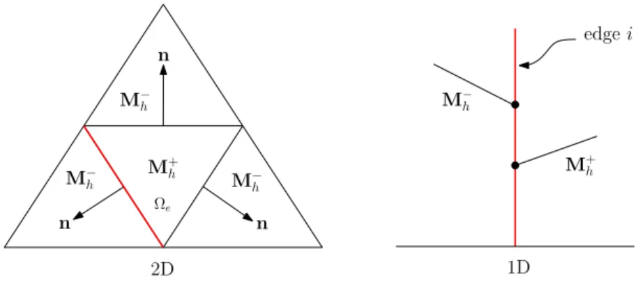
In application, the flux may not be uniquely defined along an edge since the DG method allows the numerical solution to be discontinuous along element edges, as shown in Figure 3.2. This issue is addressed by employing the concept of numerical

flux ˆf(Mh), evaluated using the local Lax-Friedrich flux.

Calculations are then performed over the master triangular element . This master

element ˆΩe represents a given physical element whose position in Cartesian

coordi-nates has been transformed to the local coordinate system ξ = (ξ1, ξ2), illustrated in

Figure 3.3. To integrate the terms of the discrete weak form of the model equation over the master triangular element we use numerical quadrature which allows us to integrate polynomials exactly. The full set of equations for all elements can then be expressed as a system of ordinary differential equations. We discretize these ordinary

(32)

M+ h M−h M−h M−h n n n M−h M+ h 2D 1D edgei Ωe

Figure 3.2: Discontinuities of the the solution M_h at the interior and exterior edge

of i. [9]

differential equations in time using explicit, strong-stability preserving Runge-Kutta schemes, which are a series of forward Euler steps in time.

Further detail on the implementation using a DG finite element method can be found in [8]. Ωe ˆ Ω ξ2 ξ1 y x (x1, y1) (x2, y2) (x3, y3) Te: (x, y)→(ξ1, ξ2) (1,−1) (−1,−1) (−1,1)

Figure 3.3: Transformation of the physical element to the master triangular element. [9]

(33)

CHAPTER 4

APPLICATIONS WITH A LAKE ERIE TEST CASE

This chapter presents the test case applied in this study on an unstructured mesh of Lake Erie. The process of application is described and results are presented. All tests were run on a 64-bit DELL Optiplex 990 machine with 16 GB RAM and dual quad-core 3.40 GHz Intel i7-2600 processors.

4.1

Model Execution

Both the SWAN model and the DG–WAVE model were run in hind cast for several months of 2010 and 2011. Key input files are described below, and significant wave height results for three months are presented. SWAN was run using an input file specifying commands and the freely available SWAN executable. DG–WAVE was run using a graphical user interface (GUI) constructed in the C.H.I.L. DG–WAVE’s

main parameters are directional spreading s and wave growth W which are set to

0.5 and 0.007 for these simulations, respectively. After performing several sensitivity analyses on the SWAN input parameters, the appropriate values and commands were determined to run SWAN as consistently to DG–WAVE as possible. SWAN was run with wind fields turned on as the only input grid. All hind casts were run on the same computational mesh with the same input commands, edited only for the individual

(34)

run times as altered by days within the month. The time step for both the windfields and output were ten minute intervals and the runtimes as determine by month are set to the exact beginning and end of each month plus an additional three day ramping period to account for the incorporation of a non-zero initial condition on the lake surface on the actual first day of the month. The ramping period thus provides a slow build up of dynamic conditions from a zero initial condition.

4.1.1

Unstructured Mesh

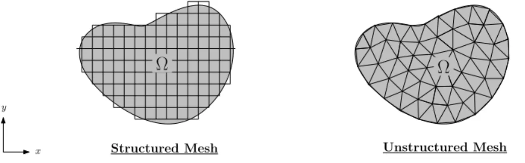
Applying a hydrodynamic model to any body of water requires the use of a mesh of the domain of the area, or a digital map of the the water body. The alignment of this mesh defines the horizontal and vertical geometry in terms of the coastline latitude and longitude as well as bathymetric depths. Two types of meshes exist for these purposes; structured meshes utilize equally-sized resolution, while unstructured meshes vary the resolution throughout the domain. Structured meshes can be ben-eficial for simplicity while unstructured meshes offer a much better ability to adapt and capture realistic boundaries, as shown in 4.1.

y

x

Ω

Structured Mesh Unstructured Mesh

Ω _Ω

Figure 4.1: Example of a structured mesh and an unstructured mesh fitting to a curving coast line.

(35)

An unstructured mesh was used for this application because of its advantageous qualities in more accurately capturing resolution along coastline areas, allowing results to be more accurate. The same mesh was used for both models. The unstructured mesh of Lake Erie utilized for both the SWAN and DG–WAVE simulations was cre-ated by ADMESH, an Advanced mesh generator for coastal ocean modeling [1], [10]. The mesh contains 2,433 elements and 1,335 nodes. The maximum element size is 5 kilometers and the minimum element size is 4 kilometers, as shown in Figure 4.2. [4]

NDBC 45005

EC 45132

EC 45142

Figure 4.2: Unstructured Mesh of Lake Erie created using ADMESH with buoy loca-tions

4.1.2

Wind Fields

An accurate wave simulation hinges significantly on the quality of the input forcing fields; most importantly, in this case, wind fields. The input wind speed that drives

(36)

SWAN isU10, the wind speed at 10 meter elevation from the surface, but is converted

to the friction velocityu∗ before being used in computations within the program. Both

SWAN and DG–WAVE utilized the same wind input files for their computations to ensure a balanced comparison of the two models. These wind input files were created using data gathered from twenty seven meteorological stations provided by the Nation Oceanic and Atmospheric Association (NOAA). These twenty seven stations were selected from the available forty seven in Lake Erie based on factors such as recording frequency and ease of data interpolation. The stations record a variety of data however the wind direction and wind speed are the only data sets that will be utilized. After data is gathered, an interpolation program transforms the raw data to a common

interval of time and interpolates the u and v (x and y) components, respectively, of

the wind field onto the mesh file for Lake Erie at ten-minute intervals. [8]

4.2

Results

DG WAVE and SWAN hindcast simulations were run over three seperate months: June 2011, August 2011, and October 2011. Significant wave height data was collected as well as a measurement of computation time for each simulation. Control data was acquired from three Lake Erie buoys for validation. Figures 4.4, 4.5, and 4.6 provide results for each of the three months where significant wave heights produced by SWAN and DG–WAVE are plotted together against buoy data. Each month’s data is shown broken down into 3 plots, one for each buoy location.

4.2.1

Buoy Data

The accuracy of the results produced by SWAN and DG–WAVE can be deter-mined by assessing their correlation to actual buoy data gathered from three unique

(37)

meteorological recording buoys in Lake Erie. The buoys utilized for this study are Buoy 45005, Buoy 45132, and Buoy 45142, which are owned and maintained by Na-tional Data Buoy Center and Environment Canada, respectively. These particular three buoys are the only meteorological recording buoys currently stationed in Lake Erie. The locations of the buoys are shown in Figure 4.3. Accelerometers aboard the buoys record the vertical displacement over time at intervals of typically 20 minutes and from this data significant wave height can be derived.

Buoys 45005

45132

45142

(38)

4.2.2

Significant Wave Height Results

The first set of hindcast results presented are for the month of June 2011. We can see from a time-series comparison with the buoy data that SWAN and DG–WAVE are very well correlated both with each other and with the actual significant wave height at each buoy. DG–WAVE very accurately captures the event on June 2, as well as the event on June 20. At some points, DG–WAVE slightly underestimates significant wave height after a large event. The second set of hindcast results presented are for the month of August 2011. Again the significant waves heights produced by SWAN and DG WAVE are well correlated with each other as well as with the control data. DG–WAVE captures the event on August 8 very nicely as well as the event on August 25, though overestimating slightly during the large event from August 28-30. During this month DG WAVE has very few underestimations of significant wave height and is fact better correlated to many of the low dips than SWAN. Lastly, October 2011 is presented in hindcast. The time-series comparisons show similar results to the previous two months, with both SWAN and DG–WAVE very accurately representing the events beginning on October 14 and ending on October 24 for all three locations.

4.2.3

Run Time Comparison

A main focal point of this study is the investigation of the computational efficiency of both SWAN and DG–WAVE. As previously mentioned, the computational time of a wave model has a huge impact on the model’s effectiveness and overall functionality. By decreasing the computational cost of a model, the model runs faster and is more available for application by a variety of users. In order to make this comparison the Lake Erie hindcasts, results from which were presented in the previous section,

(39)

6/1 6/2 6/3 6/4 6/5 6/6 6/7 6/8 6/9 6/10 6/11 6/12 6/13 6/14 6/15 6/16 6/17 6/18 6/19 6/20 6/21 6/22 6/23 6/24 6/25 6/26 6/27 6/28 6/29 6/30 7/1 0 0.2 0.4 0.6 0.8 1 1.2 1.4 Hs ( m ) 6/1 6/2 6/3 6/4 6/5 6/6 6/7 6/8 6/9 6/10 6/11 6/12 6/13 6/14 6/15 6/16 6/17 6/18 6/19 6/20 6/21 6/22 6/23 6/24 6/25 6/26 6/27 6/28 6/29 6/30 7/1 0 0.2 0.4 0.6 0.8 1 1.2 1.4 Hs ( m ) Buoy45005 DG wave model SW AN 6/1 6/2 6/3 6/4 6/5 6/6 6/7 6/8 6/9 6/10 6/11 6/12 6/13 6/14 6/15 6/16 6/17 6/18 6/19 6/20 6/21 6/22 6/23 6/24 6/25 6/26 6/27 6/28 6/29 6/30 7/1 0 0.2 0.4 0.6 0.8 1 1.2 1.4 1.6 Hs ( m ) 6/1 6/2 6/3 6/4 6/5 6/6 6/7 6/8 6/9 6/10 6/11 6/12 6/13 6/14 6/15 6/16 6/17 6/18 6/19 6/20 6/21 6/22 6/23 6/24 6/25 6/26 6/27 6/28 6/29 6/30 7/1 0 0.2 0.4 0.6 0.8 1 1.2 1.4 1.6 Hs ( m ) Buoy45132 DG wave model SW AN 6/1 6/2 6/3 6/4 6/5 6/6 6/7 6/8 6/9 6/10 6/11 6/12 6/13 6/14 6/15 6/16 6/17 6/18 6/19 6/20 6/21 6/22 6/23 6/24 6/25 6/26 6/27 6/28 6/29 6/30 7/1 0 0.2 0.4 0.6 0.8 1 1.2 1.4 1.6 1.8 2 2.2 H s ( m ) Buoy 45142 DG SWAN 6/1 6/2 6/3 6/4 6/5 6/6 6/7 6/8 6/9 6/10 6/11 6/12 6/13 6/14 6/15 6/16 6/17 6/18 6/19 6/20 6/21 6/22 6/23 6/24 6/25 6/26 6/27 6/28 6/29 6/30 7/1 0 0.2 0.4 0.6 0.8 1 1.2 1.4 1.6 1.8 2 2.2 H s ( m ) Buoy45142 DG wave model SW AN 31

(40)

8/1 8/2 8/3 8/4 8/5 8/6 8/7 8/8 8/9 8/10 8/11 8/12 8/13 8/14 8/15 8/16 8/17 8/18 8/19 8/20 8/21 8/22 8/23 8/24 8/25 8/26 8/27 8/28 8/29 8/30 8/31 9/1 0 0.2 0.4 0.6 0.8 1 1.2 1.4 1.6 1.8 H s ( m ) 8/1 8/2 8/3 8/4 8/5 8/6 8/7 8/8 8/9 8/10 8/11 8/12 8/13 8/14 8/15 8/16 8/17 8/18 8/19 8/20 8/21 8/22 8/23 8/24 8/25 8/26 8/27 8/28 8/29 8/30 8/31 9/1 0 0.2 0.4 0.6 0.8 1 1.2 1.4 1.6 1.8 H s ( m ) Buoy45005 DG wave model SW AN 8/1 8/2 8/3 8/4 8/5 8/6 8/7 8/8 8/9 8/10 8/11 8/12 8/13 8/14 8/15 8/16 8/17 8/18 8/19 8/20 8/21 8/22 8/23 8/24 8/25 8/26 8/27 8/28 8/29 8/30 8/31 9/1 0 0.4 0.8 1.2 1.6 2 2.4 2.8 H s ( m ) 8/1 8/2 8/3 8/4 8/5 8/6 8/7 8/8 8/9 8/10 8/11 8/12 8/13 8/14 8/15 8/16 8/17 8/18 8/19 8/20 8/21 8/22 8/23 8/24 8/25 8/26 8/27 8/28 8/29 8/30 8/31 9/1 0 0.4 0.8 1.2 1.6 2 2.4 2.8 H s ( m ) Buoy45132 DG wave model SW AN 8/1 8/2 8/3 8/4 8/5 8/6 8/7 8/8 8/9 8/10 8/11 8/12 8/13 8/14 8/15 8/16 8/17 8/18 8/19 8/20 8/21 8/22 8/23 8/24 8/25 8/26 8/27 8/28 8/29 8/30 8/31 9/1 0 0.2 0.4 0.6 0.8 1 1.2 1.4 1.6 1.8 2 Hs ( m ) 8/1 8/2 8/3 8/4 8/5 8/6 8/7 8/8 8/9 8/10 8/11 8/12 8/13 8/14 8/15 8/16 8/17 8/18 8/19 8/20 8/21 8/22 8/23 8/24 8/25 8/26 8/27 8/28 8/29 8/30 8/31 9/1 0 0.2 0.4 0.6 0.8 1 1.2 1.4 1.6 1.8 2 Hs ( m ) Buoy45142 DG wave model SW AN 32

(41)

10/10 10/2 10/3 10/4 10/5 10/6 10/7 10/8 10/9 10/10 10/11 10/12 10/13 10/14 10/15 10/16 10/17 10/18 10/19 10/20 10/21 10/22 10/23 10/24 10/25 10/26 10/27 10/28 10/29 10/30 10/31 11/1 0.4 0.8 1.2 1.6 2 2.4 2.8 3.2 Hs ( m ) 10/10 10/2 10/3 10/4 10/5 10/6 10/7 10/8 10/9 10/10 10/11 10/12 10/13 10/14 10/15 10/16 10/17 10/18 10/19 10/20 10/21 10/22 10/23 10/24 10/25 10/26 10/27 10/28 10/29 10/30 10/31 11/1 0.4 0.8 1.2 1.6 2 2.4 2.8 3.2 Hs ( m ) Buoy45005 DG wave model SW AN 10/10 10/2 10/3 10/4 10/5 10/6 10/7 10/8 10/9 10/10 10/11 10/12 10/13 10/14 10/15 10/16 10/17 10/18 10/19 10/20 10/21 10/22 10/23 10/24 10/25 10/26 10/27 10/28 10/29 10/30 10/31 11/1 0.4 0.8 1.2 1.6 2 2.4 2.8 3.2 Hs ( m ) 10/10 10/2 10/3 10/4 10/5 10/6 10/7 10/8 10/9 10/10 10/11 10/12 10/13 10/14 10/15 10/16 10/17 10/18 10/19 10/20 10/21 10/22 10/23 10/24 10/25 10/26 10/27 10/28 10/29 10/30 10/31 11/1 0.4 0.8 1.2 1.6 2 2.4 2.8 3.2 Hs ( m ) Buoy45132 DG wave model SW AN 10/10 10/2 10/3 10/4 10/5 10/6 10/7 10/8 10/9 10/10 10/11 10/12 10/13 10/14 10/15 10/16 10/17 10/18 10/19 10/20 10/21 10/22 10/23 10/24 10/25 10/26 10/27 10/28 10/29 10/30 10/31 11/1 0.4 0.8 1.2 1.6 2 2.4 2.8 3.2 3.6 4 H s ( m ) 10/10 10/2 10/3 10/4 10/5 10/6 10/7 10/8 10/9 10/10 10/11 10/12 10/13 10/14 10/15 10/16 10/17 10/18 10/19 10/20 10/21 10/22 10/23 10/24 10/25 10/26 10/27 10/28 10/29 10/30 10/31 11/1 0.4 0.8 1.2 1.6 2 2.4 2.8 3.2 3.6 4 H s ( m ) Buoy45142 DG wave model SW AN 33

(42)

were rerun using identical input files and measured for computational time. Three simulations were performed for SWAN and DG–WAVE for each month. The measured times for each month were then averaged, resulting in the values shown in Figure 4.2.3. More detailed results from simulations performed for May through October of 2011 are presented in Table 4.1.

Figure 4.7: Computational time comparisons from simulations run with SWAN vs DG WAVE for June, August, and October 2011

To summarize, the average of the average CPU time for SWAN is 3.26 hours or 195.9 minutes, while the average of the average CPU time for DG WAVE is only 6.24 minutes. From these results we can see that the average CPU time for DG– WAVE simulation is consistently around 30 times faster than the average CPU time for SWAN simulation. Considering the level of accuracy achieved in the significant wave height results, the typical CPU times for DG–WAVE prove very promising for potential future applications of the model.

(43)

Table 4.1: Computational times in minutes for the months of May through October 2011.

Month Run SWAN Run Time (Minutes) DG–WAVE Run Time (Minutes)

May 1 204 6.22 May 2 200 6.41 May 3 208 6.29 June 1 207 6.31 June 2 206 6.28 June 3 199 6.27 July 1 191 6.25 July 2 194 6.24 July 3 191 6.20 August 1 208 6.31 August 2 207 6.30 August 3 207 6.28 September 1 181 6.14 September 2 181 6.12 September 3 180 6.10 October 1 202 6.25 October 2 206 6.22 October 3 202 6.19

(44)

CHAPTER 5

CONCLUSION AND FUTURE WORK

This chapter concludes with finishing remarks and discussion of future work. Taking results from Chapter 4 into consideration, we can see that both DG–WAVE and SWAN perform well when validating significant wave height against actual buoy data. Assuming accurate wind information can be acquired, both models are capable of producing relatively accurate significant wave height results. The correlation be-tween the significant wave height values from the two models shows that the accuracy of DG–WAVE is on par with that of a widely used wave model such as SWAN. While SWAN has a very broad set of capabilities, our computational time results prove that DG–WAVE is a more efficient method of modeling for an application such as this. While there is much work to be done, this study shows that DG–WAVE is a robust and accurate wave model which has the potential to be developed into a high powered and efficient computational tool for coastal water studies. With the development of a comprehensive model, domains such as the Great Lakes could be more efficiently studied with great accuracy and largely decreased cost.

One limitation of DG–WAVE is that the model formulation is based on the as-sumption that waves are governed by linear deep water theory, which could be of

(45)

some concern for producing accurate results in the near-shore area of the mesh. Fu-ture work will include developing the model to accomodate shallow water effects using a phase-resolving approach to account for shoaling, wave runup, and calculation of near-bottom velocities. Other aspects of future work include coupling DG–WAVE with a three-dimensional, time-dependent DG circulation model for high-resolution simulations as well as investigating ways to expand the model for use with a wider variety of applications.

(46)

(47)

BIBLIOGRAPHY

[1] Colton Conroy. Admesh: An advanced mesh generator for hydrodynamic models. Master’s thesis, The Ohio State University, Columbus, Ohio, 2010.

[2] John R. Bennett David J. Schwab and Paul C. Liu. Application of a simple

numerical wave prediction model to Lake Erie. Journal of Geophysical Research,

89(C3):3586–3592, May 1984.

[3] John R. Bennett David J. Schwab and Edward W. Lynn. A two-dimensional lake wave prediction system. Great Lakes Environmental Research Laboratory, 1984.

[4] David Dibling. Development and validation of a high-resolution, nearshore model for lake erie. Master’s thesis, The Ohio State University, Columbus, Ohio, 2012. [5] Mark A. Donelan. A simple numerical model for wave and wind stress prediction. Report, National Water Research Insitute, Burlington, Ontario, September 1977. [6] M. Donelan K. Hasselmann S. Hasselmann G.J. Komen, L. Cavaleri and

P.A.E.M. Janssen. Dynamics and Modelling of Ocean Waves. Cambridge

Uni-versity Press, 1 edition, 1996.

[7] Leo H. Holthuijsen. Waves In Oceanic and Coastal Waters. Cambridge

Univer-sity Press, 1 edition, 2007.

[8] Angela Nappi. Development and application of a discontinuous galerkin-based wave prediction model. August 2013.

[9] Angela Nappi. Development and application of a discontinuous galerkin-based wave prediction model. Master’s thesis, The Ohio State University, Columbus, Ohio, 2013.

[10] Dustin West. Admesh: A graphical user interface for an advanced mesh generator for coastal ocean modeling. Master’s thesis.