Performance Evaluation of Techniques for Identifying
Abnormal Energy Consumption in Buildings
MEGHA GAUR 1, STEPHEN MAKONIN 2, IVAN V. BAJIĆ 2, AND ANGSHUL MAJUMDAR 1
1Department of Computer Science, Indraprastha Institute of Information Technology Delhi, New Delhi 110020, India 2School of Engineering Science, Simon Fraser University, Burnaby, BC V5A 1S6, Canada
Corresponding author: Megha Gaur ([email protected])
This work was supported in part by the India-Canada Centre for Innovative Multidisciplinary Partnerships to Accelerate Community Transformation and Sustainability, Canadian Networks of Centres of Excellence (IC-IMPACTS NCE) in Canada and in part by the Department of Science and Technology (DST) in India.
ABSTRACT Energy consumption in buildings has steadily increased. Buildings consume more energy than necessary due to suboptimal design and operation. Apart from retro-fitting, not much can be done with the design of the existing building, but the operation of the building can be improved. Ignoring or failing to fix the faults can lead to problems like the higher cost in excess energy usage or premature component failure. At the same time understanding, identifying, and addressing abnormal energy consumption in buildings can lead to energy savings and detection of faulty appliances. This paper investigates two key challenges found in energy anomaly detection research: 1) the lack of labeled ground truth and 2) the lack of consistent performance accuracy metrics. In the first challenge, labeled ground truth is imperative for training and benchmarking algorithms to detect anomalies. In the second challenge, consistent performance accuracy metrics are crucial to quantifying how well algorithms perform against each other. There exists no publicly available energy consumption dataset with labeled anomaly events. Therefore, we propose two approaches that help in the automatic annotation of the ground truth data from publicly available datasets: a statistical approach for short-term data and a piecewise linear regression method for long-term data. We demonstrate these approaches using two publicly available datasets called Dataport (Pecan Street) and HUE. Using different existing accuracy metrics, we run a series of experiments on anomaly detection algorithms and discuss what metrics can be best used for consistent accuracy testing amongst researchers. In addition, while providing the source code, we also release an anomaly annotated dataset produced by this source code.
INDEX TERMS Abnormal energy consumption, accuracy metrics, anomaly detection, baseline generation, ground truth annotation, performance evaluation.
I. INTRODUCTION
Commercial and residential buildings together consume a significant fraction of the total energy use. In the USA, this fraction was as high as 41% [1] while in India it was 37% [2] in 2016. Electricity powers our heating and cooling systems, our ovens and stoves, lighting, and our refrigerators and freezers within these buildings. Any appliance or equipment in disrepair, while operating, can lead to high energy costs.
Studies done by the U.S. Environmental Protection Agency (EPA) suggest that buildings waste an average of 30% of the energy they consume [3]. A 2012 analysis done by Lawrence Livermore National Laboratory (LLNL) sug-gested the USA is only 39% energy efficient [4]. Strategies to help increase the energy efficiency in buildings are needed,
The associate editor coordinating the review of this manuscript and approving it for publication was Monjur Mourshed.
especially in the case of older buildings where appliances have a higher likelihood of failing.
One strategy, anomaly detection, is to identify appli-ances in a state of disrepair or used improperly. Identifying these types of anomalies can create alerts to either repair an appliance or to suggest a more optimal use. Anomaly detection, also referred to as outlier detection, deals with find-ing patterns in the signal that are abnormal, unexpected, or interesting.
A. DEFINING ANOMALIES
An anomaly can be defined in several different ways and there are many different types of anomalies. For example, an anomaly can be vacation days [5] because these are days with low total consumption as compared to typical, non-vacation days. Power utilities can define an anomaly as
unexpected power consumption that results in a customer contacting customer service to complain.
The textbook definition of an outlier as defined by Harkins [6] is as follows, ‘‘An outlier is an observation that deviates so much from other observations as to arouse suspicion that it was generated by a different mechanism.’’ Anomaly detection is widely used in different applications domains like credit card fraud detection in banking and finance, insurance or health care, telecommunications [7], intrusion detection in cyber security [8], [9], sensor net-works [10], military surveillance, discovering criminal behavior, to name a few. Chandola et al. [11] presents a comprehensive review of anomaly detection techniques in general, whereas Sodemann et al. [12] reviews techniques used for outlier detection in automated surveillance. In this paper, our focus is on detection of anomalous power con-sumption in residential buildings.
The energy consumption can be labelled as anomalous or non-anomalous only when it is compared with historical data. Anomalies are broadly classified into three types: point anomalies, collective anomalies, and contextual anomalies. 1) POINT ANOMALY
When an individual observation is considered anomalous with respect to the rest of the data.
2) SEQUENTIAL OR COLLECTIVE ANOMALY
When a sequence of observations are anomalous with respect to the rest of the data.
3) CONTEXTUAL ANOMALY
When a observation is considered normal with respect to one context but not in another context. For example, consumption behaviour on weekdays versus weekends.
Power utility companies can define anomalies as calls into customer service where customers report their bills with unexpectedly high consumption charges. Some exam-ples include an appliance left on by mistake, a compres-sor failure in a fridge, a basement renter using different appliances (e.g., plug-in heater), the purchase and usage of a new appliance, guests visiting for a long period of time (holiday season), and having the thermostat set-points too low/high as seasons change. Abnormal energy consumption pattern could also imply a malicious activity like energy theft [13].
B. CHALLENGES WITH ANOMALY DETECTION
Anomaly detection poses several different challenges that can be domain specific. For the problem of detecting anomalies in energy usage there are several such challenges includ-ing: no clear definition of normal vs abnormal, imprecise boundaries between normal and abnormal behaviour, lack of ground truth, lack of a unified metric used for performance evaluation, and evolving normal behaviour of the data [11].
One of the most significant barriers to design and test anomaly detection algorithms is the lack of labelled ground
truth data. Metadata that labels the occurrences of anomalies (and their type) in datasets simply does not exist and creating such datasets is onerous and expensive. Therefore, we will present an alternative way to test the accuracy of anomaly detection algorithms using a basic statistical approach that gives us the anomaly scores at hour-level and day-level.
Additionally, from a review of anomaly detection algo-rithms [14]–[16], we have found there is no consistent way to measure the accuracy of these algorithms. In order to compare one algorithm against another there must be a standard set of metrics used to measure and report the accuracy results. In this work, we review and compare the metrics used to mea-sure the accuracy of various anomaly detection algorithms using an automatically generated baseline.
C. PAPER CONTRIBUTIONS
As we mentioned above, the lack of ground truth has ham-pered the development of advanced algorithms as there is no clear way of testing their performance accuracy. To address the challenges faced by testing anomaly detection algorithms our paper provides:
1) two novel methods to generate labelled (i.e., ground truth) data for abnormal energy consumption in build-ings for both short-range and long-range data;
2) the source code used to generate labelled data in a standard way;
3) a publicly available dataset of anomalies found in our experiments, so researchers can use this data directly; 4) a comprehensive review of all the different accuracy
measures used; and
5) a framework and discussion on how accuracy methods work when compared to each other and what perfor-mance metrics to use.
There is a lack of publicly available anomaly dataset for ground truth testing – why use an algorithmic method to label anomalies? We could invite a group of domain experts to manually label existing datasets; however, this would be expensive, time consuming, and would not guarantee accurate ground truth. The manual labelling of anomalies is highly subjective and there would most likely be disagreement amongst the knowledge experts. Having an algorithmic way of labelling anomalies would provide dataset that can be used for performance testing in a timely and consistent way.
All this creates new insight as to how we can develop algo-rithms that detect anomalies and measure their performance. D. PAPER ORGANIZATION
The remainder of the paper is organized as follows. Rel-evant literature is reviewed in the section II. Proposed techniques used to annotate anomalous and non-anomalous events using short-term data and long-term data are presented in sectionIII. The description of datasets used in our work and evaluation of different performance accuracy metrics used in existing works can be found in sectionIV. Finally, the results and concluding remarks are presented in sectionsVand VI
II. LITERATURE REVIEW
A. ANOMALY DETECTION IN BUILDING ENERGY CONSUMPTION
Anomalies are often considered as noise or error but they may contain some important information which, on rectification, could lead to better energy utilization [17]. The research com-munity has addressed the detection of abnormal energy con-sumption in several ways. An extensive review of techniques using machine learning and statistical methods for general outlier detection has been provided by [18]–[20]. We give a brief review of methods used specifically for identifying abnormal energy consumption in buildings.
1) STATISTICAL METHODS
Statistical anomaly detection techniques use statistical prop-erties of the normal activities to build norm profile and employ statistical tests to determine the deviation of the observed data from the norm profile [21]. These methods are based on the assumption of known underlying distribution of observations [6], [22]. Any observation that deviates from the model assumption is flagged as an anomaly.
a: PROXIMITY BASED METHODS
These methods compute the neighbourhood for each data point using a distance metric. An analysis of the neighbour-hood is done to determine whether a point is an anomaly or not. These techniques are simple and do not make any prior assumption about the underlying data distribution. The k-Nearest Neighbor (k-NN) method requires euclidean dis-tances between all data insdis-tances, leading to exponential computation growth. Therefore, several different variations ofk-NN were developed to improve runtime [15], [23]–[25].
Ramaswamy et al. [23] introduced an optimized k-NN by
using techniques such as partitioning the data into cells. This helped in speeding up the processing as the distance for only the cells with data points lesser than a pre-defined threshold
was computed. Wettschereck [26] used a supervised k-NN
method to classify a new exemplar based on the majority classification of the nearest neighbours. The weighted voting power decreased as the distance increased. Belallaet al.[15] proposed unsupervised clustering based anomaly detection, which flagged data points lying outside tight clusters as anomalous. They first created a low dimensional representa-tion of each day’s energy consumprepresenta-tion and usedk-NN density estimation based approach to compute anomaly scores by comparing lower dimensional representation of various days. These scores ranked days based on how anomalous they were. Arjunanet al.[14] proposed a multiuser energy consumption monitoring and anomaly detection technique that uses an unsupervised k-medoid clustering algorithm based on Parti-tioning Around Mediods (PAM) and also uses neighbourhood information to adjust the anomaly scores.
b: PARAMETRIC METHODS
Statistical parametric methods assume the known underly-ing distribution of observations [6], [22]. They annotate as
outliers those observations that deviate from model assump-tion. These methods allow the model to be evaluated quickly for new instances and are suitable for large datasets. Seem [16] uses a statistical approach (mean and standard deviation) to identify anomalous days. He first groups days based on energy consumption profile (weekends/weekdays) and then computes anomaly score for each day using gen-eralized extreme studentized deviate (ESD) many-outlier procedure that was proposed by Rosner [27]. Wang and Xiao [28] uses a strategy based on principal component analysis (PCA) to detect and diagnose the faults in air han-dling units (AHU). Fault detection using PCA is based on the intuition that anomalous readings are far away from the centre (mean/median) of the principal components of sensor data. Principal components with lower variance are preferred because, on such dimensions the normal objects are likely to be close to each other and outliers deviate from the majority.
Narayanswamy et al. [29] compares the correlation, PCA
and rules based methods [30] with a data mining technique proposed by them called model, cluster and compare (MCC) to detect faults in variable air volume boxes in large com-mercial buildings. Zhanget al. [5] proposed a regression, entropy and clustering based method to detect anomalous days for accurate demand response (DR) prediction. They define anomalous days as vacation days, when energy con-sumption mainly consists of automatic cycling of appliances. The regression method obtained the best test results. c: NON-PARAMETRIC METHODS
The model of normal (non-anomalous) data is learned from the input data rather than assuming ita priori. Since fewer assumptions about the data are made, these models are more flexible and autonomous. Histogram based anomaly detec-tion [31] is a nonparametric statistical technique that involves building a histogram using the feature values in the training data. The size of the bins plays a key role in determining the accuracy of the technique. If the test instance falls in any of the bins of the histogram, it is considered normal, else anomalous. Desforgeset al.[32] proposed a semi-supervised statistical technique that used kernel functions to estimate the probability density function of the normal instances. Any observation lying in the low probability area of this function is anomalous. Neural networks have also been employed by researchers to model and predict the energy consumption in a solar building [33]. Karatasou et al. [34] show how the performance of neural networks used for building’s energy prediction can be improved by using some statistical proce-dures. Brown et al.[35] used kernel regression method to predict the power output by using the weighted average of nearby neighbourhoods. They outperformed neural networks significantly when the training data used was for 6 months or less.
2) MACHINE LEARNING-BASED METHODS
Most commonly used machine learning methods for outlier detection employ ensemble learning. Ensemble learning
methods [36] are based on the intuition that a single algo-rithm can not detect variety of anomalies present in the data. Initially, ensemble learning builds several homogeneous or heterogeneous base learners and then uses combination techniques to combine their outputs. Ensemble methods for anomaly detection can be categorized as sequential or independent [37]. In the former approach, different algo-rithms are applied sequentially whereas in the latter approach, the results are combined from execution of different
algo-rithms in parallel. Araya et al. [38] proposed ensemble
anomaly detection (EAD) framework combining several dif-ferent learners, which in turn relied on pattern and/or predic-tion based approaches. They evaluated a combined threshold value (ensemble threshold) depending on the optimal sen-sitivity and specificity. References [33], [34], [39] investi-gate an unsupervised autoencoder-based ensemble method in detecting anomalies in building energy data. Some hybrid approaches [40]–[42] have also been developed, which com-bine statistical, neural and machine learning approaches. Chou and Telaga [43] proposed a real-time prediction model, neural network auto regression (NNAR) combining time series autoregressive integrated moving average (ARIMA) and artificial neural network (ANN). They used the 2-sigma rule for anomaly detection and compare their proposed method with standard ARIMA.
B. BASELINE
This paper addresses the problem of unavailability of proper benchmarking data as well as a unified set of metrics to evalu-ate the performance of various outlier detection schemes. The accuracy measures to evaluate different anomaly detection approaches developed so far are not well defined. Public ground truth is not readily available; therefore, existing work uses the following ways to create a baseline:
• manual inspection of hundreds of traces of the dataset by a domain expert,
• artificial injection of anomalies in the dataset, and • discussion with building managers or owners to verify
the anomalies.
All the above mentioned strategies either rely on third-party account or create privacy concerns and are intrusive. The manual inspection of hundreds of different traces of data seems impractical and inefficient, and is subject to human error (e.g., memory recall). Many studies also employ syn-thetic datasets or artificial anomalies with the objective to successfully uncover them using their proposed methods. This technique may not be able to model a realistic distribu-tion of anomalies. Another way to have the true informadistribu-tion about the anomalies is by asking the users or home owners to review their activities on a fixed time basis.
Khanet al.[44] used outlier detection schemes to uncover the injected anomalies in their work. Whereas, [10], [14], [29] asked the building managers to manually verify anomalies in their dataset. The work done by [45] discusses the anomalies uncovered (high true positive rate and low false positive) by their method through visual inspection. The authors however,
claim to not be able to analyze the missed anomalies (false negatives) due to the lack of labelled data. Bellalaet al.[15] use help from building administrators to select a threshold k, such that top-k days are labelled as anomalous.
III. PROPOSED METHODS
A. NOMENCLATURE
The following symbols are used in the remainder of the paper.
d day of the month
g number of groups with similar score
h hour of the day
m number of monthly data points per house
n number of houses in the dataset
s a segment in segmented or piecewise linear
regres-sion
X weekday or weekend data matrix with hours of the
day as rows and days of the month as columns with entriesxh,d ∈ X
Z z-score matrix with entrieszh,d ∈ Z
δ user or building administrator-defined threshold
µh hourly mean
σh hourly standard deviation
label1 positive side of the anomaly
label2 negative side of the anomaly
score a row vector of anomaly scores
pos a list of indices of anomaly scores sorted in descend-ing order
B. METHODOLOGY
One concern that power utilities have is to reduce the number of customer complaint calls when they receive a high elec-tricity bill. Informing a customer in advance, proactively, can be a positive experience for customers.
For cases like these, we have devised an approach that would detect anomalies from weekly or monthly data. This approach gives power utilities a flexibility to input the desired threshold,δsuch that if the z-score is above or belowδ stan-dard deviations (δ-SDs), the observation would be considered anomalous and marked as ‘1’. This flexibility can help the utilities to easily segregate customers based on the degree of their anomalous activities. Customers with high anomaly scores are likely to get high electricity bills in the future, hence they have a higher chance of making a complaint call.
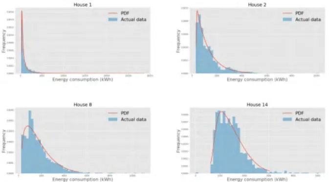
The energy consumption (kWh) histograms of different houses in Dataport dataset were fitted with best (least sum of squared error) probability density functions. The set of proba-bility density functions used to fit the histograms were alpha, beta, gamma, chi squared, boxcox, rayleigh, skewnorm, log-norm, loggamma, weibull, exponorm and logistic. The details of these continuous distributions can be found in the statistics package of SciPy.1 Fig.1 shows histograms of four differ-ent houses with ids 1,2,8 and 14 fitted with four differdiffer-ent probability density functions that are alpha, exponnorm, beta
FIGURE 1. Probability density functions that best-fit four different houses in short-range dataset. The best-fit distribution for house ids starting from top-left quadrant, going in clockwise direction (1,2,14,8) are alpha, exponnorm, skewnorm and beta respectively.
and skewnorm. As can be seen in fig.1, there is no particular distribution that best fits all the houses in the dataset. There-fore, a distribution function can not be generalized for all the houses.
We know that Chebyshev’s inequality [46] guarantees that atleast 75% of data lies within 2-SDs of the mean or in other words for a thresholdδ, we can say that atmost (100/δ2)% of values that are outside (δ-SDs) are considered as anomalous. This theoretical bound is much weaker than the actual but that is expected. We propose two approaches to generate ground truth anomaly labels based on the size of the available data: short-range and long-range.
Algorithm 1 Statistical Method to Generate Ground-Truth Anomalies for Short-Range Data
Require: n,m, δ fori = 1:ndo forj = 1:mdo calculateµh,σh calculate zh,d = xmh,d−µh σh (1) label1h,d ←zh,d> δ label2h,d ←zh,d<−δ
labelh,d ←label1h,d | label2h,d label1d ←Ph(label1h,d) label2d ←Ph(label2h,d) score←label1d−label2d
[pos]←Rankdays based onscore Findg groups of days with samescore,
fork = 1:gdo
calculate zd ←Ph:zh,d>δzh,d (2)
sortdays in each groupgbased onzdscores update pos
end for end for
normalize score← score−min
max−min (3)
end for
Return score,pos
1) SHORT-RANGE DATA
This method is based on the z-scores. A z-score is a measure of how many standard deviations a data point is from the sample mean. The intuition behind a separate algorithm for a short-range data is the uncertainty in the consumption pattern and also unavailability of long-range datasets due to privacy concerns.
For this method, we separate the monthly data into groups of days with similar energy consumption profiles. For resi-dential houses, we create two groups, weekdays and week-ends. The energy consumption profile of days belonging to the same group would be similar. We then perform the following steps for each group.
1) For each data group matrix X, whose (d,h)th entry represents the amount of energy consumed aththhour of the day anddthday of the month, we compute the hourly meanµh and standard deviation σh across all days in the group.
2) We then compute the z-score for each element in the matrixXusing eq. (1) in Algorithm1.
3) The threshold for anomaly is taken as an input by
the user. The values in matrix Z are compared with
the threshold. If the value of |zh,d| >δ, then the label
is marked as ‘1’ (abnormal) else ‘0’ (normal). The obtained label values are stored in binary matrices,
label1h,dandlabel2h,d, respectively. The label for each
hour of the daylabelh,d is obtained by performing a
logical ‘or’ operation betweenlabel1h,dandlabel2h,d.
4) For the day-level score, we sum the rows of ground truth matrix obtained at hour-level. We then subtract the scores inlabel1h,d and label2h,d matrices to get
the net score. The value of net score determines the extent of abnormal energy consumption on a particular day. The positive net score indicates the positive side of anomaly, that is when the energy consumption is more than usual, whereas the negative score indicates the abnormally low energy consumption.
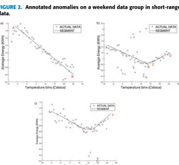
5) The annotated positive and negative label on a weekend group is shown in fig. 2. This figure shows energy consumption of House1 from Dataport on weekend days. The red circles indicate positive anomaly whereas the black star represents negative anomaly. As we are more interested in the positive side of the anomaly, we sort the days in the descending order of the day-level anomaly scores.
6) We create groups of days with the same anomaly score to resolve the ranking conflict between days with the same score.
7) For each group, we compute the sum of z-score values that are greater than the desired thresholdδ, as shown in eq. (2).
8) Finally, we normalize the scores using min-max nor-malization using eq. (3) in Algorithm1, where the max and min values are taken from the data group matrixX.
9) The algorithm outputs pos which represents days in
FIGURE 2. Annotated anomalies on a weekend data group in short-range data.
FIGURE 3. Prediction of energy usage by segmented linear regression.
Three different case scenarios of energy consumption using segmented linear regression are: a) unsegmented linear regression b) segmented linear regression with one breakpoint, and c) segmented linear regression with two breakpoints. Actual energy consumption is shown in blue dots whereas the segments that best fits the data are shown in black.
scorewhich defines the extent to which these days are anomalous. A day is anomalous if it is assigned ascore
greater than 0. 2) LONG-RANGE DATA
Long-range energy usage and temperature data gives a better understanding of the user consumption pattern through the annual seasons. With more data, it is easier to know the consumption trend of a user.
For this case, we have used annual energy and temperature data from different houses. This data is sampled at hour-level. The correlation coefficient between outside temperature and energy consumption as shown in fig. 3a is 0.955. The high correlation between these two variables is the foundation of this approach. The graphs shown in fig. 3 represent three different cases of energy consumption with respect to the outside temperature. During winters, the energy consump-tion increases as the temperature decreases due to invariable heating needs. This is represented in fig. 3 by the negative slope segment ‘AB’. Similarly, during summers, as the tem-perature increases the energy consumption also increases due to cooling loads as can be seen by the positive slope segment ‘CD’. The energy used for cooling or heating of the building is referred to as temperature-sensitive usage. The energy used by computers, lights or appliances not sensitive to the outside
temperature is referred to as temperature-insensitive usage. This kind of usage can be identified by a segment with a near-zero slope, ‘EF’. A house could have a cooling or a heating appliance, or both, or none, therefore a single linear regression function is not adequate to cover all the cases. This is why the segmented linear regression is necessary, as described below.
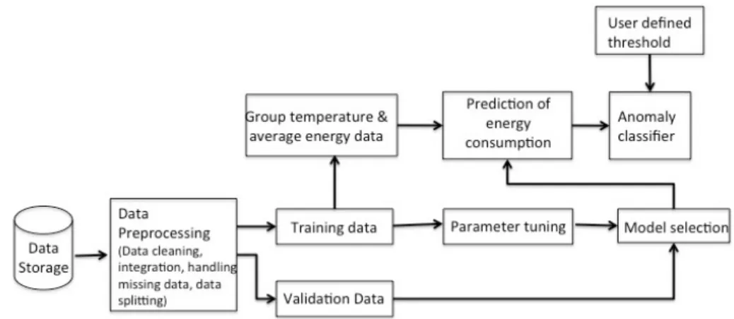
1) The first step is to prepare the dataset for training. Preprocessing involves cleaning the data, removing inconsistent and redundant timestamps, adding miss-ing timestamps, addmiss-ing missmiss-ing energy consumption values and integrating hourly temperature data. The missing values are usually caused by a hardware or a software failure of the measurement device. The missing energy values were replaced by the values of previous or next year’s data corresponding to the same timestamp. For cases where the previous and next year data was not available, the average of previous and next hour of the current year was used.
2) After the data is preprocessed, it is split into training and validation sets in the ratio of 9:1 respectively. A single instance or sample at hth hour was selected from every 10 samples to create the validation set. The remaining samples were used for the training set. 3) Next, the training set is used for model selection or
model training. Grid search is used to train the model. The parameters in the case of pure, unsegmented linear regression are also tuned in this step. The parameters tuned include the set of breakpoints in the case of segmented regression, regression coefficients and con-stants. The optimal value of the breakpoint is found such that the coefficient of determination,R2shown in eq. (4) is maximum. In this equation,yi refers to the
observed data point,y¯is the mean of all the observed data points andfirepresents the predicted power
con-sumption. R2=1− P i(yi−fi)2 P i(yi− ¯y)2 (4) 4) The model is tested on the validation set. In a sce-nario where no heating or cooling is used, the unseg-mented linear regression may perform better than the segmented one.
5) The sorted temperature values are grouped together such that each group has sufficient number of energy consumed data points. Since the frequency distribution of data points at the maximum and minimum tempera-ture values will be minimum, we merge the groups such that each group has sufficient (in our case atleast 20) number of data points.
6) The grouped training data is partitioned based on the parameters obtained from the test on the validation set. The number of segments and the breakpoints are optimally chosen depending on the bestR2value. 7) For each segment in the partitioned training dataset,
FIGURE 4. Block diagram for annotating ground truth anomalies using long-range data. best learned linear regression coefficients and constants
values.
8) To determine the anomalous data point, we compute the z-score of the difference between the actual and predicted energy consumption as we did in step 2 of Algorithm 1. We compare the z-score with δ, as we
did in step 3 of Algorithm 1 to obtain two binary
column vectors,label1handlabel2h representing the
positive and negative side of the anomaly respectively. To obtain the finallabel, we performed a logical ‘or’ operation betweenlabel1 andlabel2 generated for each timestamp.
9) Using these binary anomaly labels for the grouped training dataset, we identify the corresponding anoma-lous data in the actual hourly readings and annotate the ground truth. On the grouped training dataset, figure5
shows the normal or non-anomalous data (blue dots), regression model (shown by straight lines) and anoma-lies (red stars). We may observe annotated anomaanoma-lies (red star) closer to the straight line than the normal data (blue dot) because data points are an average of energy consumption values lying in the same bin. So, it may be possible for one of the value in the averaged group has z-score of the difference between actual and predicted energy greater than a threshold whereas the rest of the values be closer to the straight line. The correlation coefficients between the average yearly energy con-sumption and the outside temperature corresponding to the three regression line segments are 0.6545, 0.8440 and 0.7937 respectively.
IV. EXPERIMENTAL SETUP
A. DATASET
1) DATAPORT DATASET
The first dataset used is the publicly available Dataport (Pecan Street) dataset with NILMTK [47]. For our work, we are using the NILMTK format data which consists of 239 houses located in Texas, US. Each house has meter-level as well as appliance-level data, which are sam-pled at 1 minute intervals. We are using two months (April
FIGURE 5. Annotation of anomalous observations in long-range data.
and May) of meter-level data from nine houses. For con-venience, we consider 30 days in both months. The aver-age temperature in these two months was 19◦C and 23◦C, respectively. Short-range data analysis III-B.1was applied to this dataset. We have used houses with ids 1, 2, 3, 4, 5, 8, 11, 12 and 14. The house ids which were discarded due to missing data are 6, 7, 9, 10, 13. For each month, the data was grouped based on the day types, that is, days of the week with similar energy consumption profiles were grouped together. Therefore, for each month we have weekdays consisting of 22 days and weekends consisting of eight days. Aggregation of both groups of data takes place at an hour-level. Hence, the size of the weekday dataset per month would be (24×22) and that of weekend would be (24×8).
2) HUE DATASET
The second dataset used is collected from different residential houses located in Burnaby in British Columbia, Canada [48]. This dataset has meter-level electricity consumption val-ues which are sampled at each hour. The data is collected over a period of three years, ranging from January 2015 to January 2018. We have used five houses from this dataset with house ids 3, 4, 5, 6, 7. However, there are more than five
houses in this dataset. Hourly temperature data was included in the dataset, which we used to detect abnormal energy consumption from yearly data. The integration of weather and energy consumption data was done to find the correlation between them. Long-range data analysis III-B.2was applied to this data.
B. PERFORMANCE METRICS
Performance metrics allow us to measure how accurately a detection algorithm identifies an anomaly in the energy consumption pattern. It is important to measure how effective an approach is in the classification task of anomalous vs non-anomalous behaviour of energy signals. The notion of anomaly score is used to quantify the extent of anomalous behaviour in the energy signals. High anomaly score means high degree of anomalousness. For example, the work done by [16], uses robust statistical methods to determine if the cur-rent day’s energy consumption is significantly diffecur-rent from the previous days’ energy consumption. They use generalized extreme studentized deviate (ESD) as an outlier identification method [27]. To quantify how far and in which direction an outlier is from the mean value of non-outlier observations, a modified z-score was used.
We have compiled a list of performance evaluation metrics that have been used to measure the performance accuracies in the majority of the anomaly detection methods. These are explained in the remainder of this section.
1) TRUE POSITIVE RATE (TPR)
This is also commonly known as sensitivity, or outlier detection rate, or recall. TPR is the proportion of correctly identified positive classes from the total possible positive con-ditions, that are true positives (TP) and false negatives (FN). In the context of anomaly detection, TPR measures the frac-tion of anomalous events identified by a given method.
TPR= TP
TP+FN, (5)
The research done by [5], [38] have used TPR as their perfor-mance evaluation metric. In sectionV, TPR is reported as the mean of all TPR values obtained from different houses. 2) TRUE NEGATIVE RATE (TNR)
Also known as specificity, TNR is the proportion of correctly identified negative classes from the total possible negative conditions, that are true negative (TN) and false positive (FP). In the context of anomaly detection, TNR measures the fraction of non anomalous events identified by a given method. References [15], [38] have used TNR to measure the accuracy of their testing. Both TPR and TNR aim to reveal how accurately a technique has identified the true nature of a given sample, that is whether it is anomalous or not.
TNR= TN
TN+FP, (6)
3) FALSE POSITIVE RATE (FPR)
FPR refers to the rate of false alarms or fall-out, which means misclassifying some non-outliers as outliers. It has been applied as an accuracy metric in [5], [38], and [49].
FPR=1−TNR, (7)
4) F1SCORE
F1score or F-measure is widely used in the field of informa-tion retrieval for measuring search, document classificainforma-tion and query classification performance. It indicates the retrieval effectiveness of the system and is defined as the harmonic mean of the precision defined in eq. (9) and recall (TPR).F1
score is defined in eq. (8).
F1= 2∗prec∗recall
prec+recall , (8)
Precision and Recall (TPR), on the other hand are the traditional performance metrics used to evaluate the quality of the information retrieval system [50], [51], and are also widely used to measure the performance of outlier detection schemes. Precision (prec) is the fraction of relevant instances among the retrieved instances as defined in eq. (9). High precision is when the algorithm returns more relevant results than irrelevant ones. On the other hand, recall (or TPR ), as defined in eq. (5) is the fraction of relevant instances that have been retrieved over total relevant instances. High recall is when the algorithm returns most of the relevant results. Equation (10) expressesF1score in terms of TP, FP and FN.
prec= TP
TP+FP, (9)
F1=
2TP
2TP+FN+FP, (10)
Reference [9] uses precision and recall as metrics to compare and evaluate the performance of outlier detection schemes on real-life and synthetic datasets.
5) JACCARD INDEX
Jaccard index, also referred to as intersection over union (IOU), is a metric used for comparing the similarity and diversity of sample sets. In the context of anomaly detection, this measure estimates the similarity between the two sets of data, one obtained through the anomaly detection method and other from the ground truth anomalies.
Jaccard = TP
TP+FP+FN, (11)
6) FALSE POSITIVE WHEN DETECTION RATE IS 100% (FP-100)
FP-100 is the number of false positives returned by the algo-rithm when the algoalgo-rithm has detected all the anomalous days as given in the ground truth. It can be used to compare two algorithms, suppose if a dataset has 10 known anomalies and the rank of the 10th anomaly is 17 by algorithm ‘A’ and 20 by algorithm ‘B’, then algorithm ‘A’ is better than ‘B’ because
for 100% detection rate, ‘A’ has only 7 false positives whereas ‘B’ has 10. The work by [49] have used FP-100 as a metric to evaluate the performance of their algorithm.
7) AREA UNDER CURVE (AUC)
The receiver operating curve (ROC) is commonly used to measure the performance of the classifier by plotting true positive rate against false positive rate. The area under this curve, AUC, defines the quality of the detector. AUC is often used to measure the performance of the algorithm [5], [15],
[38], [49]. The value of AUC = 1 represents a perfect
anomaly classifier whereas a value of AUC = 0.5 signifies the performance of the model to be no better than a random guess.
8) PARTIAL AREA UNDER CURVE (pAUC)
The partial area under the curve is a performance metric defined as the area within the range of specific true positive and false positive rate. It is more suitable for comparing clas-sifiers whose ROC curves cross [38]. For example, if amongst two anomaly classifiers A and B, let us say A has better true positive rate than B in a specific false positive rate range while classifier B performs better in a different false positive rate range, then we can identify a specific range relevant to the application to apply pAUC rather than AUC, which gives an overall combined metric.
9) RANK POWER
Even though Precision and Recall are widely used to measure the accuracy of anomaly detection, they still lack in some respects, mainly because they do not give any preference to the ranks, that is, how anomalous is a particular sample. As proposed by [9], rank power shown in eq. (12) evaluates the ratio of known anomalies and anomalies returned by an algorithm along with their rankings [49].
RankPower(k)= l·(l+1)
2·Pl
i=1Ri
(12) wherelis the number of outliers among topkobjects.Riis
the position of theith outlier in a rank-order list. C. IMPLEMENTATION
Algorithms used to annotate the data observations using short and long-term approaches were implemented in MATLAB. The codes to implement these methods have been made avail-able on GitHub2. The implementation of various performance metrics is also publicly available at the same site.
V. RESULTS
We conducted performance experiments on real-world pub-licly available datasets. As mentioned in section IV-A, we have used a subset of Dataport dataset [47] and the HUE dataset [48] to generate labels for short-term data (weekly or monthly) and long-term energy consumption
2https://github.com/megha89/AnomalyDetection
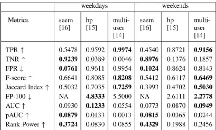
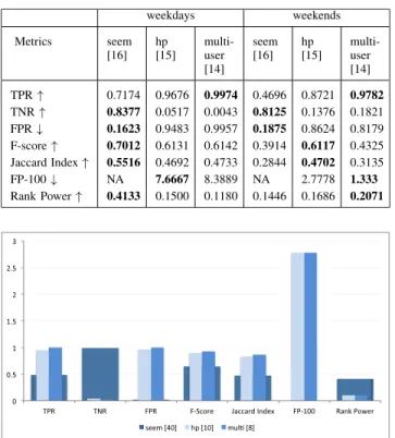
TABLE 1.Performance accuracies on weekdays and weekends on
Dataport when the threshold is 1.65-SDs.
TABLE 2.Performance accuracies on weekdays and weekends on
Dataport when the threshold is 2-SDs.
data (yearly) respectively. The ground truth labels are gener-ated for three different thresholds, that are 1.65-SDs, 2-SDs and 2.5-SDs. As the value of threshold increases, the anoma-lies become sparser.
The anomaly scores obtained using anomaly detection methods [14]–[16] are compared with the scores generated through Algorithm1. These methods which we refer to as ‘multiuser’ [14], ‘hp’ [15] and ‘seem’ [16] have been briefly discussed in sectionIIof this paper. Table1 shows a com-parison of different accuracy measures for weekdays and weekends separately, provided that the data lying outside
±1.65-SDs is considered anomalous. Similarly, Tables 2
and 3 report the accuracies of algorithms for thresholds
±2-SDs and ±2.5-SDs, respectively. The upward (↑) and downward (↓) arrows in tables1,2and3indicate the direc-tion of desirable performance according to that metric.
For both weekday and weekend groups, it can be observed
from Tables 1, 2 and 3 that [14] gives the best TPR
whereas [16] outputs the lowest TPR across all thresholds. One possible reason why [16] outputs the lowest TPR could be that they consider an upper bound on the number of potential outliers, ou. The maximum number of potential
outliers can beou< 0.5(o−1) whereois the total number of
observations. We should also note that its anomaly detection rate increases as we increase the threshold for anomalous data.
Contrastingly, in case of TNR, [16] clearly outperforms the rest in correctly identifying the normal observations from
TABLE 3. Performance accuracies on weekdays and weekends on Dataport when the threshold is 2.5-SDs.
FIGURE 6. Comparison of performance accuracies on weekdays when the
threshold is 1.65-SDs.
abnormal ones during weekdays and weekends. Furthermore, in case of false alarms or FPR, [16] again has a very low misclassification rate in comparison to others methods. After comparing TPR, TNR and FPR values, it can be concluded that the techniques [14] and [15] classified majority of the normal data as abnormal therefore maximizing TPR and FPR but minimizing TNR. Thus, only presenting a very high TPR result can be misleading if it is not accompanied with high TNR and low FPR values. All three rates are important to make an informed decision about the classification accuracy. The ability of an algorithm to return all known outliers with minimum number of false positives is captured by the metric FP-100. Here, [15] returns less false positives when detection rate is 100% than [14] in case of weekdays but vice versa for weekends. We have not mentioned the results from [16] because this method does assign a score to all the observations, therefore leading to cases where known anomalies are more than the assumed potential anomalies.
The other metric, F1 score, which is based on precision and recall, evaluates the ranking of results. From eq. (10), we observe thatF1is directly proportional to TP and inversely
proportional to the sum of FN and FP. Therefore, best F1
can only be attained with high true positives and low false positives and false negatives. On comparingF1scores across
all thresholds, we observe that when the threshold is high-est, [16] attains the bestF1score. Also, it should be noted that
as the threshold value increases, theF1score using [16] also increases but on the other hand, this score decreases for [14].
FIGURE 7.Comparison of performance accuracies on weekends when the
threshold is 1.65-SDs.
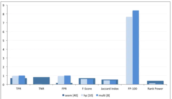
FIGURE 8. Comparison of performance accuracies on weekdays when the
threshold is 2-SDs.
FIGURE 9.Comparison of performance accuracies on weekends when the
threshold is 2-SDs.
Jaccard index as shown in eq. (11) is a metric similar to F-score. It is a statistic used to estimate the similarity of two sets of data. We use the Jaccard index values to compare the accuracy of different anomaly detection methods. Intuitively, it follows a similar trend asF1score but with lower scores.
The most commonly used metric is area under the ROC curve (AUC). After the ranked list of data is obtained from a algorithm, the user chooses a threshold, τ ∈ (0,1) declaring that the points above the threshold are anoma-lous and, the remaining normal. Each choice of value ofτ gave out a certain value of true positive and false positive. On varying this thresholdτ, different values of TPR (y-axis) and FPR (x-axis) were obtained, leading to a ROC curve.
FIGURE 10. Comparison of performance accuracies on weekdays when the threshold is 2.5-SDs.
FIGURE 11. Comparison of performance accuracies on weekends when
the threshold is 2.5-SDs.
The values for AUC presented in Table 2 were calculated
after considering thresholds from 10% to 90% with a step size of 10%. The low values of AUC is due to the low range of false positives. Though the values of TPR and FPR were high but the range across all thresholds was very low leading to low AUC.
Rank power [9] is an effective metric that meets the users’ satisfaction by factoring in the rank of the outliers. As shown in eq. (12), rank power forkobjects is the ratio of knownl
anomalies in topkdata to the ranking of thoselanomalies as returned by the algorithm. In our study, we took the value of
kas 3 because the number of anomalies returned by [16] in case of weekend data were at most 3. Tables1,2and 3show that [16] outperforms other approaches across all thresholds. From the results, we can say that the ranking of anomalies in case of [16] was more precise than the rest. We have also graphically presented the results given in the tables using overlapping bar graphs in figures6to11.
From this experiment, we can conclude that [16] outper-formed the rest of the techniques. If it had assigned scores to all the days, then it would have performed the best across all the reported metrics.
VI. CONCLUSION
In this work, we discuss the two most common problems in detecting abnormal energy consumption in buildings. The first problem is the the lack of labelled ground truth to train
supervised models, and the second is the lack of consistent performance accuracy metrics.
To mitigate the first problem, we have proposed two methods to generate labelled data for abnormal energy con-sumption in buildings. These methods are based on the size of the available dataset. For a short-term dataset, we have proposed a statistical approach that uses user-defined input as a threshold for anomaly scores. It outputs hourly and day-level binary labels and scores denoting whether the given hour is anomalous or not, and to what extent, respectively. The other method is for long-range data, where an approach based on segmented linear regression is proposed. It uses the correlation between the average temperature values and average energy consumption values to find the anomalous timestamps.
For the second problem, we studied and conducted exper-iments to evaluate different performance metrics used in the field of anomaly detection. We can therefore conclude that there is no perfect metric available that can capture all kinds of anomalous behaviour. However, the combination of TPR, TNR, FPR, Rank Power, AUC and FP-100 metrics gives a more robust and accurate view of an algorithm’s performance. The contributions made through this work are: (1) pro-posed two novel methods to generate labelled data, (2) a publicly available source code to generate labelled data, (3) a publicly available annotated dataset of anomalies, (4) a comprehensive review of different accuracy measures, and (5) a framework and discussion of what performance accuracy metrics to use.
ACKNOWLEDGMENTS
The authors would like to thank Andrew Berrisford at BC Hydro and David Campbell at SFU Statistics for their feedback, insights, and suggestions.
REFERENCES
[1] Monthly Energy Review 2018, U.S. Energy Inf. Admin., Washington, DC, USA, Jul. 2018.
[2] Annual Report 2016–2017, Bur. Energy Efficiency, Govt India, Ministry Power, New Delhi, India, 2016.
[3] Energy Efficiency in Commercial Buildings, Energy Star, U.S. Environ. Protection Agency, Washington, DC, USA, 2016.
[4] Estimated U.S. Energy Use in 2012, Lawrence Livermore Nat. Lab., Dept. Energy, Livermore, CA, USA, May 2013.
[5] Y. Zhang, W. Chen, and J. Black, ‘‘Anomaly detection in premise energy consumption data,’’ inProc. IEEE Power Energy Soc. General Meeting, Jul. 2011, pp. 1–8.
[6] D. Hawkins,Identification of Outliers. London, U.K.: Chapman & Hall, 1980.
[7] T. Fawcett and F. Provost, ‘‘Adaptive fraud detection,’’Data Min. Knowl. Discovery, vol. 1, no. 3, pp. 291–316, Sep. 1997.
[8] W. DuMouchel and M. Schonlau, ‘‘A fast computer intrusion detection algorithm based on hypothesis testing of command transition probabili-ties,’’ inProc. KDD, 1998, pp. 189–193.
[9] J. Tang, Z. Chen, A. W. Fu, and D. W. Cheung, ‘‘Capabilities of out-lier detection schemes in large datasets, framework and methodologies,’’ Knowl. Inf. Syst., vol. 11, no. 1, pp. 45–84, Jan. 2007.
[10] D. J. Hill and B. S. Minsker, ‘‘Anomaly detection in streaming environ-mental sensor data: A data-driven modeling approach,’’Environ. Model. Softw., vol. 25, no. 9, pp. 1014–1022, 2010.
[11] V. Chandola, A. Banerjee, and V. Kumar, ‘‘Anomaly detection: A survey,’’ ACM Comput. Surv., vol. 41, no. 3, p. 15, 2009.
[12] A. A. Sodemann, M. P. Ross, and B. J. Borghetti, ‘‘A review of anomaly detection in automated surveillance,’’IEEE Trans. Syst., Man, Cybern. C, Appl. Rev., vol. 42, no. 6, pp. 1257–1272, Nov. 2012.
[13] P. Jokar, N. Arianpoo, and V. C. M. Leung, ‘‘Electricity theft detection in AMI using customers’ consumption patterns,’’IEEE Trans. Smart Grid, vol. 7, no. 1, pp. 216–226, Jan. 2016.
[14] P. Arjunan, H. D. Khadilkar, T. Ganu, Z. M. Charbiwala, A. Singh, and P. Singh, ‘‘Multi-user energy consumption monitoring and anomaly detection with partial context information,’’ inProc. 2nd ACM Int. Conf. Embedded Syst. Energy-Efficient Built Environ. (BuildSys), New York, NY, USA, 2015, pp. 35–44.
[15] G. Bellala, M. Marwah, M. Arlitt, G. Lyon, and C. E. Bash, ‘‘Towards an understanding of campus-scale power consumption,’’ inProc. 3rd ACM Workshop Embedded Sens. Syst. Energy-Efficiency Buildings (BuildSys), New York, NY, USA, 2011, pp. 73–78.
[16] J. E. Seem, ‘‘Using intelligent data analysis to detect abnormal energy consumption in buildings,’’Energy Buildings, vol. 39, no. 1, pp. 52–58, 2007.
[17] O. Maimon and L. Rokach,Data Mining and Knowledge Discovery Hand-book. Secaucus, NJ, USA: Springer-Verlag, 2005.
[18] V. J. Hodge and J. Austin, ‘‘A survey of outlier detection methodologies,’’ Artif. Intell. Rev., vol. 22, no. 2, pp. 85–126, 2004.
[19] M. A. F. Pimentel, D. A. Clifton, L. Clifton, and L. Tarassenko, ‘‘A review of novelty detection,’’Signal Process., vol. 99, pp. 215–249, Jun. 2014. [20] M. Markou and S. Singh, ‘‘Novelty detection: A review—Part 1: Statistical
approaches,’’Signal Process., vol. 83, no. 12, pp. 2481–2497, 2003. [21] M. Shyu, S. Chen, K. Sarinnapakorn, and L. Chang, ‘‘A novel anomaly
detection scheme based on principal component classifier,’’ inProc. IEEE Found. New Directions Data Mining Workshop, Conjunction (ICDM), Jan. 2003, pp. 171–179.
[22] R. Pincus, ‘‘Barnett, V., and Lewis T.: Outliers in statistical data. 3rd edi-tion. J. Wiley & Sons 1994, XVII. 582 pp.,$49.95,’’Biometrical J., vol. 37, no. 2, pp. 256–256, 1995.
[23] S. Ramaswamy, R. Rastogi, and K. Shim, ‘‘Efficient algorithms for mining outliers from large data sets,’’ inProc. ACM SIGMOD Int. Conf. Manage. Data (SIGMOD), New York, NY, USA, 2000, pp. 427–438.
[24] E. M. Knorr and R. T. Ng, ‘‘Algorithms for mining distance-based outliers in large datasets,’’ inProc. 24th Int. Conf. Very Large Data Bases (VLDB). San Francisco, CA, USA: Morgan Kaufmann, 1998, pp. 392–403. [25] J. Tang, Z. Chen, A. W. chee Fu, and D. Cheung, ‘‘A robust outlier
detection scheme for large data sets,’’ inProc. 6th Pacific–Asia Conf. Knowl. Discovery Data Mining, 2001, pp. 6–8.
[26] D. Wettschereck, ‘‘A study of distance-based machine learning algo-rithms,’’ Ph.D. dissertation, Oregon State Univ., Corvallis, OR, USA, 1994. [27] B. Rosner, ‘‘Percentage points for a generalized ESD many-outlier
proce-dure,’’Technometrics, vol. 25, no. 2, pp. 165–172, 1983.
[28] S. W. Wang and F. Xiao, ‘‘AHU sensor fault diagnosis using principal com-ponent analysis method,’’Energy Buildings, vol. 36, no. 2, pp. 147–160, 2004.
[29] B. Narayanaswamy, B. Balaji, R. Gupta, and Y. Agarwal, ‘‘Data driven investigation of faults in HVAC systems with model, cluster and compare (MCC),’’ inProc. 1st ACM Conf. Embedded Syst. Energy-Efficient Build-ings, New York, NY, USA, 2014, pp. 50–59.
[30] M. Peña, F. Biscarri, J. I. Guerrero, I. Monedero, and C. León, ‘‘Rule-based system to detect energy efficiency anomalies in smart buildings, a data mining approach,’’Expert Syst. Appl., vol. 56, pp. 242–255, Sep. 2016. [31] M. Goldstein and A. Dengel, ‘‘Histogram-based outlier score (HBOS):
A fast unsupervised anomaly detection algorithm,’’ German Res. Centre Artif. Intell. (DFKI), Kaiserslautern, Germany, Tech. Rep. KI-2012, 2012. [32] M. J. Desforges, P. J. Jacob, and J. E. Cooper, ‘‘Applications of probability density estimation to the detection of abnormal conditions in engineering,’’ Proc. Inst. Mech. Eng., C, J. Mech. Eng. Sci., vol. 212, no. 8, pp. 687–703, 1998.
[33] S. A. Kalogirou, ‘‘Applications of artificial neural-networks for energy systems,’’Appl. Energy, vol. 67. nos. 1–2, pp. 17–35, Sep. 2000. [34] S. Karatasou, M. Santamouris, and V. Geros, ‘‘Modeling and predicting
building’s energy use with artificial neural networks: Methods and results,’’ Energy Buildings, vol. 38, no. 8, pp. 949–958, Aug. 2006.
[35] M. Brown, C. Barrington-Leigh, and Z. Brown, ‘‘Kernel regression for real-time building energy analysis,’’J. Building Perform. Simul., vol. 5, no. 4, pp. 263–276, 2012.
[36] Z. Zhou,Ensemble Methods: Foundations and Algorithms. London, U.K.: Chapman & Hall, 2012.
[37] C. C. Aggarwal, ‘‘Outlier ensembles: Position paper,’’SIGKDD Explor. Newslett., vol. 14, pp. 49–58, Apr. 2013.
[38] D. B. Araya, K. Grolinger, H. F. Elyamany, M. Capretz, and G. Bitsuamlak, ‘‘An ensemble learning framework for anomaly detection in building energy consumption,’’Energy Buildings, vol. 144, pp. 191–206, Jun. 2017.
[39] C. Fan, F. Xiao, Y. Zhao, and J. Wang, ‘‘Analytical investigation of autoencoder-based methods for unsupervised anomaly detection in build-ing energy data,’’Appl. Energy, vol. 211, pp. 1123–1135, 2018. [40] A. Capozzoli, F. Lauro, and I. Khan, ‘‘Fault detection analysis using data
mining techniques for a cluster of smart office buildings,’’Expert Syst. Appl., vol. 42, no. 9, pp. 4324–4338, Jun. 2015.
[41] A. Kialashaki and J. R. Reisel, ‘‘Modeling of the energy demand of the residential sector in the United States using regression models and artificial neural networks,’’Appl. Energy, vol. 108, pp. 271–280, Aug. 2013. [42] P. Singh and P. Dwivedi, ‘‘Integration of new evolutionary approach with
artificial neural network for solving short term load forecast problem,’’ Appl. Energy, vol. 217, pp. 537–549, May 2018.
[43] J. Chou and A. S. Telaga, ‘‘Real-time detection of anomalous power con-sumption,’’Renew. Sustain. Energy Rev., vol. 33, pp. 400–411, May 2014. [44] I. Khan, A. Capozzoli, S. P. Corgnati, and T. Cerquitelli, ‘‘Fault detection analysis of building energy consumption using data mining techniques,’’ Energy Procedia, vol. 42, pp. 557–566, 2013.
[45] R. Fontugneet al., ‘‘Strip, bind, and search: A method for identifying abnormal energy consumption in buildings,’’ inProc. ACM/IEEE Int. Conf. Inf. Process. Sensor Netw. (IPSN), Apr. 2013, pp. 129–140.
[46] B. Amidan, T. Ferryman, and S. Cooley, ‘‘Data outlier detection using the chebyshev theorem,’’ in Proc. IEEE Aerosp. Conf., Mar. 2005, pp. 3814–3819.
[47] O. Parsonet al., ‘‘Dataport and NILMTK: A building data set designed for non-intrusive load monitoring,’’ inProc. IEEE Global Conf. Signal Inf. Process. (GlobalSIP), Dec. 2015, pp. 210–214.
[48] S. Makonin, ‘‘HUE: The hourly usage of energy dataset for buildings in British Columbia,’’Data Brief, vol. 23, p. 103744, Apr. 2019.
[49] M. Ali, Y. S. Kwon, C. Lee, J. Kim, and Y. Kim,Current Approaches in Applied Artificial Intelligence: 28th International Conference on Indus-trial, Engineering and Other Applications of Applied Intelligent Systems. Seoul, South Korea: Springer, 2015.
[50] R. A. Baeza-Yates and B. Ribeiro-Neto,Modern Information Retrieval. Boston, MA, USA: Addison-Wesley, 1999.
[51] G. Salton, Automatic Text Processing: The Transformation, Analy-sis, and Retrieval of Information by Computer. Boston, MA, USA: Addison-Wesley, 1989.
MEGHA GAUR received the bachelor’s degree in information technology from the Bharati Vidyapeeth College of Engineering, New Delhi, India, in 2011, and the master’s degree in com-puter science from the Indraprastha Institute of Information Technology Delhi, New Delhi, India, in 2013, where she is currently pursuing the Ph.D. degree under the supervision of Dr. A. Majum-dar. Her research interests include applied machine learning, time series analysis, signal processing, forecasting, and predictive analytics in the area of energy conservation.
STEPHEN MAKONINreceived the Ph.D. degree in computing science from Simon Fraser’s Uni-versity (SFU), in 2014. He has been a Software Engineer for more than 20 years working for vari-ous local and international clients. He is currently an Adjunct Professor in engineering science with Simon Fraser University (SFU) and also a Phi-lanthropist. His research interests include com-putational sustainability and the understanding of socioeconomic issues that pertain to technological advancements. He is also the Vice Chair of the IEEE Signal Processing Soci-ety Vancouver Chapter. He is an Editorial Board Member for Nature’s Scien-tific Datajournal. He is an Expert in data engineering and world-renowned researcher in non-intrusive load monitoring (NILM) and disaggregation.
IVAN V. BAJIĆ received the B.Sc.Eng. degree (summa cum laude) in electronics engineering from the University of Natal, South Africa, in 1998, and the M.S. degree in electrical engi-neering and mathematics and the Ph.D. degree in electrical engineering from Rensselaer Polytech-nic Institute, Troy, NY, USA, in 2002 and 2003, respectively. In addition to research, teaching, and consulting in these areas, he was also involved in new media art as a Telepresence Architect for several telematic dance/ music performances, from 2009 to 2010. He is currently a Professor of engineering science with Simon Fraser University. His research interests include signal processing, machine learning, and their applications in image and video processing, coding, communications, and multimedia ergonomics.
ANGSHUL MAJUMDAR received the bache-lor’s degree from the Bengal Engineering College, Shibpur, and the master’s and Ph.D. degrees from the University of British Columbia, in 2009 and 2012, respectively. He is currently an Associate Professor with the Indraprastha Institute of Infor-mation Technology Delhi, New Delhi. He has coauthored more than 150 papers in journals and reputed conferences. He has authoredCompressed Sensing for Magnetic Resonance Image Recon-struction(Cambridge University Press). His research interests include signal processing and machine learning. He is currently serving as the Chair for the IEEE SPS Chapter’s Committee and the Chair of the IEEE SPS Delhi Chapter. He is a Co-Editor ofMRI: Physics, Reconstruction and Analysis (CRC Press).