UWB Localization System with TDOA Algorithm Using Experimental Measurements

UWB Localization System with TDOA Algorithm Using Experimental

Measurements

Abdelmadjid Maali, Abdelaziz Ouldali

Military Polytechnic School BP 17, Bordj El Bahri, Algiers, Algeria e-mail : [email protected], [email protected]

Hassane Mimoun, Geneviève Baudoin

Université Paris Est, ESIEE Paris

2 Bd Blaise Pascal, F–93162 Noisy-le-Grand Cedex e-mail : {h.mimoun, g.baudoin}@esiee.fr Abstract—This paper investigates a 2D experimental location

system based on time difference of arrival (TDOA) of ultra wideband (UWB) signals measured in line-of-sight (LOS) and non-line-of-sight (NLOS) environments. These measurements are carried out with the UWB radios PulsON 210 from Time Domain Corporation. The measured signals are collected with four antennas which are connected through cables and a power combiner to PulsON 210 receiver. After the calculation of the electric delays cables, we applied maximum energy selection with search back (MESSB) and cell averaging constant false alarm rate (CA-CFAR) algorithms to estimate the TDOA. These algorithms use the output of non-coherent energy detection (ED) receivers. The experimental results show that the performances of TDOA estimation obtained by MESSB and CA-CFAR algorithms give almost identical performances in the LOS environment, but in NLOS case, the performances of CA-CFAR algorithm are higher than those obtained by MESSB algorithm.

Keywords-Ultra wideband (UWB); time difference of arrival (TDOA); maximum energy selection with search back (MESSB); cell averaging constant false alarm rate (CA-CFAR).

I. INTRODUCTION

Impulse Radio UWB (IR-UWB) technology uses a very short pulse with a duration typically shorter than 1 nanosecond. Therefore it can achieve high resolution ranging in the order of tens of centimeters. Consequently, with its precise ranging and location estimation, it is an ideal candidate for space applications, such as tracking of Lunar/Mars rovers and astronauts [1][2].

Many methods have been applied to estimate the location of a radio source, such as received signal strength (RSS) indicators, time of arrival (TOA), time difference of arrival (TDOA) or angle of arrival (AOA). For some applications, the TDOA approach has been chosen as an ideal method for tracking since it does not require synchronization between the transmitter and receiver [1].

The methods used in [1] and [2] to estimate TDOA are classified in matched filter (MF) receivers, that operate at high sampling frequency and use complex algorithms. Energy detection (ED) receivers work at sub Nyquist sampling frequency and use low complex algorithms that make them low cost and low power consumption.

In this paper, we use the ED receivers with maximum energy selection with search back (MESSB) [3] and cell

averaging constant false alarm rate (CA-CFAR) [4] algorithms to estimate the TDOA. The algorithms are tested on measured data obtained by using a pair of UWB radio transceivers “PulsON 210” developed by the Time Domain Corporation [5].

The remainder of the paper is organized as follows. In Section II,we briefly review the state of the art of the MF and ED receivers. In Section III, the prototype system of localization is presented, and the CA-CFAR and MESSB algorithms to estimate the TDOA are described. In Section IV, mobile localization is done in ESIEE gymnasium applying TDOA algorithm. In Section V, the experimental results are analyzed. The concluding remarks and future work are given in Section VI.

II. STATE OF THE ART

TOA estimation algorithms based on MF receivers can obtain high localization precision by means of high sampling rate, which leads unfortunately to high implementation cost. On the other hand, the algorithms which use ED receivers are based on a simple architecture which can operate at very low sampling rates compared to the Nyquist rate.

In UWB receivers, the received signal is amplified by a low noise amplifier (LNA), passed through a band-pass filter (BPF) with bandwidth B as indicated in Fig. 1. In UWB ranging approaches based on the MF receivers [6], the received signal is sampled after being correlated with a reference signal as illustrated in Fig. 1 (a), and high sampling rate is used to detect the peak correlation corresponding to TOA. In the ED receivers, the filtered signal fed to an “integrate and dump” device with an integration and sampling duration as shown in Fig. 1 (b), and the TOA estimation depends on a threshold [3].

Among the algorithms based on MF receivers, a simplified version of the Maximum Generalized Likelihood (GML) algorithm has been analyzed in [6]. In [7], the authors have proposed a Low Complexity (LC) algorithm which is based on the idea of a „„noisy template‟‟. The GML algorithm provides ranging accuracies, but requires very high sampling rates which may be a major drawback in practical applications [8].

For the ED receivers, the TOA estimation problem consists of detecting the first energy cell containing the received signal energy overcomes a suitable threshold. In

[3], the MESSB algorithm based on a fixed normalized threshold has been presented. In [4], we have proposed a CA-CFAR algorithm based on an adaptive threshold comparison. Adaptive threshold techniques are used in radar detection to maintain a constant false alarm rate (CFAR) in a non stationary environment [9][10].

Figure 1. Types of UWB receivers. (a) MF receiver; (b) ED receiver.

More generally, in most applications, the goal is to achieve ranging accuracy of a meter with low-power and low-complexity algorithms [8]. In this order, the ED receiver combined with CA-CFAR algorithm, for ranging in UWB systems, constitute a better solution for these applications.

III. TDOAESTIMATION

The core equipment employed in our experiment is a pair of UWB PulsON 210 transceivers. We show in Fig. 2 one UWB radio transceiver PulsON 210. Its specifications are as follows [5]:

 Pulse repetition frequency : 9.6 MHz;  Date rates : 9.6~0.15Mbps ;

 Center frequency : 4.7 GHz ;

 Bandwidth : 3.2 GHz, [3.1-6.3] GHz ;

 Effective Isotropic Radiated Power (EIRP) : -12.8 dBm ;

 Power consumption : 6.5 W ;

 Dimensions : 16.5 cm x 10.2 cm x 5.1 cm.

Figure 2. PulsON 210 UWB.

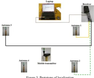
Our prototype system is based on “One-Receiver-Four-Antennas” as indicated in Fig. 3, where four antennas are connected through a power combiner to one UWB receiver using three different cables with precisely calibrated delays. Therefore, three delayed versions of the received UWB pulse are obtained at the single receiver. In our experimentation, we used only three cables because the length of the cables does not enable us to confine the four received signals in the frame duration (104 ns). Consequently, the measurements are divided into two phases. The first phase relates to the acquisition of the signals collected by antennas 1, 2 and 3. In the second phase, the received signals measurements are carried out by antennas 1, 4 and 3. This is realized by the connection of the green cable (dashed line) to antenna 4 as shown in Fig. 3.

Figure 3. Prototype of localization.

The purpose of our system is the measurement of the distances between the reception antennas and the transmitter, which is equivalent to the measurement of TOA ( , ) as indicated in the example of Fig. 4. However, if the system is not synchronized, we must rather measure relative times of arrival, after we carry out the difference to eliminate the unknown initial time . It is also necessary to determine the electric delays caused by the cables ( ,

).

A. TOA estimation with CA-CFAR and MESSB algorithms

As considered previously, before calculating the TDOA we calculate initially relative TOA (t1, t2, t3 and t4), where

, . In this section we describe the estimate of the relative TOA by CA-CFAR and MESSB algorithms. These algorithms use the output of energy detector as shown in Fig. 5 and Fig. 6. The integrator output samples can be expressed as

Where n{1,2,...,Nb} denotes the sample index. Nb is the

number of samples contained in a given time frame. The resulting samples are employed in our modified approach based on CA-CFAR technique as illustrated in Fig. 5. Where the samples (cells) are sent serially into a tapped delay line of length , excluding guard cells (the guard cells duration is chosen larger or equal to the channel mean delay [11]). The samples correspond to the reference cells and the test cell .

Figure 5. Block diagram of ED receiver employing CA-CFAR approach.

The cell averaging (CA) detector gives an alarm when the value of the test cell, , exceeds , where T is a scaling factor and

is the CA of the reference cells. The arrival time of the first sample crossing the respective threshold value is estimated as TOA [4], i.e.,

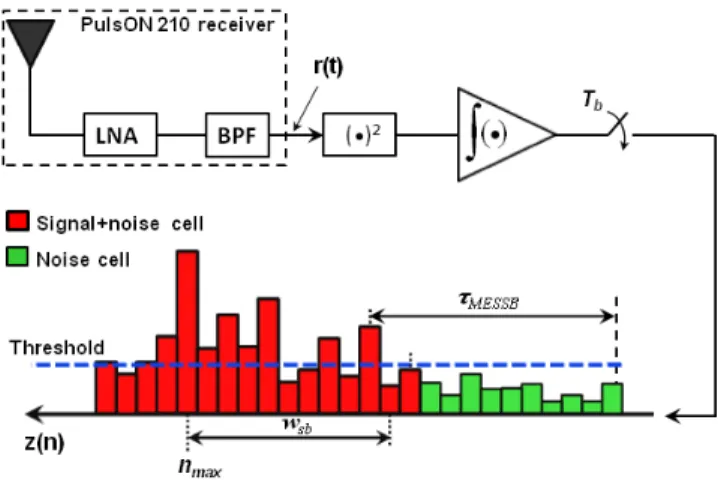
For the MESSB algorithm, the energy samples prior to the maximum should be searched as shown in Fig. 6. The TOA estimate with thresholding and backward search is then given [3]

where , the threshold is a function of the minimum and maximum values of

Figure 6. Block diagram of ED receiver employing MESSB algorithm.

The optimal value of the normalized threshold is experimentally chosen, denotes search-back window in number of samples and .

IV. MOBILE TRASMITTER LOCALIZATION

We study in this section the TDOA localization algorithm. But let us start first by the description of the localization experiment set-up. Firstly, we have a PulsON 210 transmitter fixed on a wooden support for mobility. Secondly, four antennas with known positions are mounted on a wooden support. The four static receiving antennas and the PulsON 210 transmitter were approximately 1.5 m high. These antennas are connected through a power combiner (PS4-7) to PulsON 210 receiver using three different cables with precisely calibrated delays. The PulsON 210 receiver is connected to the Laptop through standard Ethernet cable to communicate the received signals for the user as indicated in Fig. 7.

Figure 7. UWB TDOA localization experiment set-up.

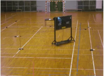
For the environment of localization, we place the four antennas at places quite selected in the space of the ESIEE gymnasium. This choice is dictated by the used cables length

and the reference antenna position as shown in Fig. 8. The cables lengths which are connected to the antennas 1, 2 (4) and 3 are 2 m, 10 m and 13.5 m, respectively.

Figure 8. Environment and prototype of localization.

A. Localization algorithm

We describe in this section the used algorithm for the mobile transmitter localization where we are interested in the 2-D localization. Let be the mobile station (transmitter) position, be the position of ith_receiving antenna and an estimate of the distances difference between and

We note M the number of antennas, the propagation velocity of the signals and an estimate of the TDOA. If we fix antenna 1 at the position , then we can estimate the position of the mobile by the following matrix form [2] : where and

Where , and M = 4 in our case. To evaluate the performances of CA-CFAR and MESSB algorithms to estimate the TDOA as well as the algorithm of localization, we proceed as follows: The transmitter trajectory contains 26 positions, and for each position of the trajectory we carry out 10 measurements of the received signal, what gives thirty values of TDOA per position and in total we obtain 780 values of TDOA.

Figure 9. Environment of localization.

The coordinates of the antennas Ant1, Ant2, Ant3 and Ant4 are measured in meters and are respectively as follows:

. We show in Fig. 9 the environment of localization.

V. EXPERIMENTAL RESULTS

To analyze the performances of the CA-CFAR and MESSB algorithms in the estimate of the TDOA and in localization, we use the Mean Absolute Error (MAE)

and Root Mean Square Error (RMSE) respectively.

For the calculation of the energy blocks , we choose the three following values of the parameter : ,

and . The experiment is made in LOS and NLOS cases. The remainder of the parameters is given as follows:

 N = 50 (Number of reference cells) for Tb = 0.5 ns

and Tb = 1 ns ;

 N = 26 for Tb = 2 ns ;

 Ng = 6 ns (Guard cells duration) ;

 wsb = 8 ns (search-back window for MESSB). A. LOS case

In LOS case, there are no obstacles between the receiving antennas and the transmitter antenna. The UWB signals received through three receiving antennas from the mobile transmitter antenna are shown in Fig. 10.

Figure 10. UWB signals received through three receiving antennas.

-2 0 2 4 6 8 10 -2 0 2 4 6 8 10 X(m) Y (m ) Ant1 Ant2 Ant4 Ant3 Target trajectory Antenna 1 Antenna 2 Transmitter Receiver Antenna 4 Antenna 3

MAE versus scaling factor T and the normalized threshold for the algorithms CA-CFAR and MESSB respectively, are given in Fig. 11. We observe that the performances obtained for the two algorithms are almost identical. For the two algorithms, the curves decreases quickly for the weak thresholds, then the curves converge towards constants. Furthermore, this figure clearly shows that the obtained results are close to the MAE theoretical limit .

Figure 11. MAE versus thresholds detection. (a) : MESSB algorithm; (b) : CA-CFAR algorithm.

Now we give in table I the performances of the two algorithms for the optimal thresholds and for two orientations 1 and 2 of the antennas. We study the effect of the antennas orientations, because when two antennas at the same elevation are rotated so the flat sides of the antennas face one another, radiation performance will be approximately 6 dB higher than when the antennas are edge-on [5]. We show that there exists a weak difference in performances between the antennas orientations 1 and 2, this is due to the fact that these algorithms are not sensitive to the 6 dB average losses caused by the orientations of the antennas. This table illustrates that CA-CFAR algorithm gives better results except for , because the number of reference cells is insufficient (N = 50). The results in table I also show, that the RMSE increases exponentially with the increase of the Tb.

TABLE I. Performances comparison between MESSB and CA-CFAR algorithms.

MAE (cm) RMSE (cm)

MESSB CA-CFAR MESSB CA-CFAR Tb = 0.5 ns Direction 1 5.08 5.45 12.75 13.25 Direction 2 5.09 5.6 12.79 13.85 Tb = 1 ns Direction 1 9.63 9.51 29.12 27.93 Direction 2 9.77 9.41 29.22 27.26 Tb = 2 ns Direction 1 19.60 19.50 95.45 87 Direction 2 19.34 19.30 90.64 89.92 B. NLOS case

In the preceding case, the receiving antennas and the mobile transmitter have a LOS condition, where the SNR is higher than 20 dB. Now, a metallic obstacle is placed between the mobile transmitter and antenna 2 in order to create an NLOS channel as indicated in Fig. 12. An example of a signal in such environment is given in Fig. 13.

Figure 12. Metallic obstacle between the mobile transmitter and the receiving antenna 2.

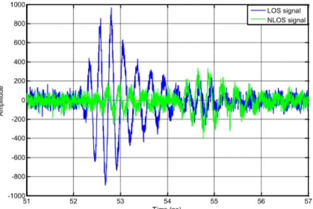
We show in Fig. 13 and Fig. 14 that the received impulse by antenna 2 in NLOS case is attenuated and delayed compared to that received in LOS case. We also show that it is followed by a more powerful reflected impulse by the floor that can cause an additional positive error to the estimate of the relative TOA.

Figure 13. Comparison between LOS/NLOS received signals. (a): LOS received signal, (b): NLOS received signal.

0 0.02 0.04 0.06 0.08 0.1 0.12 0 0.05 0.1 0.15 0.2 0.25 0.3 MAE (m) T (b) Tb = 2 ns Tb = 1 ns Tb = 0.5 ns 0 0.02 0.04 0.06 0.08 0.1 0.12 0 0.05 0.1 0.15 0.2 0.25 0.3 MAE (m) Normalized threshold (a) Tb = 2 ns Tb = 1 ns Tb = 0.5 ns 0 20 40 60 80 100 120 -2000 -1000 0 1000 2000 Time (ns) (a) Amplitud e 0 20 40 60 80 100 120 -2000 -1000 0 1000 2000 Time (ns) (b) Amplitud e Impulse of the reflected path Impulse of the direct path

Figure 14. Zoom of the selected zones in Fig. 13.

Figure 15. MAE versus thresholds detection in LOS/NLOS situations. (a) : MESSB algorithm, (b) : CA-CFAR algorithm.

We only consider in this section the MAE and we study the following cases: and with the same algorithms of TDOA estimation and the same parameters. The obtained results are given in Fig. 15. This figure clearly shows that the CA-CFAR algorithm gives better performances than the MESSB algorithm in NLOS situations. This is due to the fact that the CA-CFAR uses an adaptive threshold which detects the attenuated signals, and the MESSB detects the impulse of the reflected path instead of the impulse of the direct path which is much attenuated. Also, Fig. 15 shows that in NLOS situation, the MESSB algorithm gives the same performances for and

. This is due to the fact that the duration of the reflected impulse is lower than the duration of the LOS impulse as indicated in Fig. 14. But for CA-CFAR algorithm, the obtained performances are different for

and because the algorithm detects the weak signals.

VI. CONCLUSION AND FUTURE WORK

In the present paper, the performances of UWB experimental location system in LOS/NLOS environments have been investigated. For ranging, low complexity CA-CFAR and MESSB algorithms for relative TOA estimation are used. These algorithms are based on the use of the output of non-coherent energy detection receivers. For location estimation, TDOA algorithm is used. The system of location is based on the use of UWB radios PulsON 210 from Time Domain Corporation. Experimental results have shown that the MESSB and CA-CFAR algorithms give almost identical performances in the LOS environment. But in NLOS environment, CA-CFAR algorithm gives better results. As future work, the comparison between the two approaches can be carried out on signals measured in a dense multipath environment.

REFERENCES

[1] J. Ni, D. Arndt, P. Ngo, C. Phan, K. Dekome, and J. Dusl, “Ultra-Wideband Time-Difference-Of-Arrival High Resolution 3D Proximity Tracking System,” in Proc. IEEE Position Location and Navigation Symposium (PLANS), Indian Wells, CA, USA, pp. 37 - 43, May 2010. [2] J. Ni and R. Barton, “Design and Performance Analysis of a UWB

Tracking System for Space Applications,” in Proc. IEEE/ACES Int. Conf. on Wireless Communications and Applied Computational Electromagnetics, pp. 31- 34, April 2005.

[3] I. Guvenc and Z. Sahinoglu, “Threshold based TOA estimation for impulse radio UWB systems,” in Proc. IEEE Int. Conf. UWB (ICU), Zurich, Switzerland, pp. 420-425, Sep. 2005.

[4] A. Maali, A. Mesloub, M. Djeddou, G. Baudoin, H. Mimoun, and A. Ouldali, “Adaptive CA-CFAR threshold for non coherent IR-UWB energy detector receivers,” IEEE Communications Letters, Vol. 13, No. 12, pp. 1-3, December 2009.

[5] System Analysis Module User's Manual PulsON 210 UWB Reference Design, Time Domain Corporation, P210-320-0102B, Aug 2005. [6] J. Y. Lee and R. A. Scholtz, „„Ranging in a dense multipath

environment using a UWB radio link,‟‟ IEEE J Select Areas Commun, Vol. 20, pp. 1677–1683, 2002.

[7] S. Gezici, Z. Tian, G. B. Biannakis, and H. Kobayashi, „„Localization via Ultra-Wideband Radios, A look at positioning aspects of future sensor networks,‟‟ IEEE Signal Processing Magazine, pp. 70-84, July 2005.

[8] Z. Shahinoglu, S. Gezici, and Ismail Guvenc, "Ultra-wideband Positioning Systems : Theoretical Limits, Ranging Algorithms, and Protocols," Cambridge University Press, 2008.

[9] A. Farrouki and M. Barkat, “Automatic censoring CFAR detector based on ordered data variability for nonhomogeneous environments”,

IEE Proceedings, Radar, Sonar Navigation, Vol. 152, No. 1, pp. 43-51, February, 2005.

[10] C.-M. Cho and M. Barkat, „„Moving ordered statistics CFAR detection for nonhomogeneous backgrounds,‟‟ IEE PROCEEDINGS-F, Vol. 140, No. 5, pp. 284 -290, October 1993

[11] B. R. Mahafza, “Radar Systems Analysis and Design Using MATLAB,” Chapman & Hall/CRC, 2000.

51 52 53 54 55 56 57 -1000 -800 -600 -400 -200 0 200 400 600 800 1000 Time (ns) Amplitud e LOS signal NLOS signal 0.02 0.04 0.06 0.08 0.1 0.12 10-1 100 Normalized threshold (a) MAE (m) 0.02 0.04 0.06 0.08 0.1 0.12 10-1 100 T (b) MAE (m) Tb = 1ns (LOS) Tb = 1ns (NLOS) Tb = 2ns (LOS) Tb = 2ns (NLOS) Tb = 1 ns (LOS) Tb = 1 ns (NLOS) Tb = 2 ns (LOS) Tb = 2 ns (NLOS)