Firm Growth and Liquidity Constraints: A Dynamic Analysis

Faculdade de Economia

da Universidade de Coimbra

(GEMF)

Av. Dias da Silva, 165 – 3004-512 COIMBRA, PORTUGAL

gemf@fe.uc.pt http://gemf.fe.uc.pt

BLANDINA OLIVEIRA & ADELINO FORTUNATO

Firm Growth and Liquidity Constraints: A Dynamic Analysis

ESTUDOS DO GEMF

N.º 7 2005

PUBLICAÇÃO CO-FINANCIADA PELA FUNDAÇÃO PARA A CIÊNCIA E TECNOLOGIA

Impresso na Secção de Textos da FEUC COIMBRA 2005

Firm Growth and Liquidity Constraints:

A Dynamic Analysis

Blandina Oliveira1 (ESTG, Polytechnic Institute of Leiria) Adelino Fortunato (FEUC and GEMF, University of Coimbra)

March 1, 2005

Abstract

Using a large unbalanced panel data set of Portuguese manufacturing firms surviving over the period from 1990 to 2001, the purpose of this paper is to examine whether liquidity constraints faced by business firms affect firm growth. We use a GMM-system to estimate a dynamic panel data model of firm growth tha t incorporates cash flow as a measure of liquidity constraints and persistence of growth. The model is estimated for all size classes, including micro firms. Our findings suggest that smaller and younger firms have higher growth-cash flow sensitivities tha n larger and more mature firms. This is consistent with the suggestion that financial constraints on firm growth may be relatively more severe for small and young firms. Finally, firms that were small and young and strongly liquidity-constrained at the beginning of the sample period exhibited more persistent growth than those that were large and old and weakly liquidity-constrained. These results have significant policy implications.

Keywords: firm size, firm growth, liquidity constraints, GMM estimator, panel data.

JEL classification codes: L11, G32, C23.

1

Please address correspondence to: Blandina Oliveira, Escola Superior de Tecnologia e Gestão, Instituto Politécnico de Leiria, Morro do Lena–Alto Vieiro APARTADO 4163, 2411–901 LEIRIA, PORTUGAL. Tel.: +351 244820300. Fax: +351 244820310. Email: blandina@estg.ipleiria.pt.

1. Introduction

The availability and cost of finance is one of the factors which affects the ability of a business to grow (Binks and Ennew, 1996:17). The growth of firms, especially small and young firms, is constrained by the quantity of internally generated finance available. Butters and Lintner (1945:3) provide some of the earliest research to support this theory. They conclude that “(m)any small companies – even companies with promising growth opportunities – find it extremely difficult or impossible to raise outside capital on reasonably favourable terms” and that most small firms finance their growth almost exclusively through retained earnings. Recent empirical evidence indicates that the wedge between the cost of internal and external finance may be large for small firms. In relation to this, the financing constraints theory also complements recent research that emphasizes how access to finance affects firm formation, survival and growth2. In effect this research combines two strands of economics literature, that of the firm growth literature and that of the investment literature.

This paper applies dynamic panel data techniques to an extended firm growth specification that also includes persistence of chance and liquidity constraints proxied by cash flow, and employs the financing constraint literature to explain the dynamics of the growth of the firms. This study makes significant contributions to the literature on the dynamics of firm growth. Fir st, we investigate the effects of internal finance on firm growth in the context of surviving Portuguese manufacturing firms. The goal is to assess whether stylized facts of firm growth might be better explained by taking into account the link between financial constraints and firm growth. This differs from the large body of literature that has focused on traditional firm growth analysis, attempting to explain the relationship between firm size, age and growth. Second, our dynamic model of firm growth with liquidity constraints also addresses the effect of persistence of chance or serial correlation on firm growth. Third, we consider an unbalanced panel data set that covers all size classes, including the very smallest firms. Fourth, because we may expect that different size categories may face differences when attempting to access external finance we split our sample by firm size and firm age. Finally, we apply the dynamic panel data techniques developed by Blundell and Bond (1998), which is known as the GMM-system estimator. The GMM methods control for biases due to unobserved firm-specific effects and lagged endogenous variables.

2

See, for example, Evans and Jovanovic (1989) on financing constraints and entrepreneurial choice and Holtz-Eakin, Joulfaian, and Rosen (1994) on liquidity constraints and entrepreneurial survival.

The paper is organized as follows. Section 2 presents an overview of the literature on firm growth and financial constraints, whilst Section 3 reports a dynamic firm growth model subject to liquidity constraints and testable hypotheses. Section 4 describes the sample used and presents some descriptive statistics, and Section 5 reports the regression results and examines the robustness of our findings. Finally, Section 6 summarizes our findings and their policy implications.

2. Dynamics of firm growth and liquidity constraints

Recent studies of the relationship between firm size and growth with more detailed data sets have overturned the conclusion of Gibrat’s law (Gibrat, 1931), also known as LPE, which holds that firm size and growth are independent3. Studies by Evans (1987), Hall (1987), and Dunne and Hughes (1994) show that the growth rate of manufacturing firms and the volatility of growth is negatively associated with firm size and age. Based on this and other empirical evidence, Geroski (1995) infers a stylized result where both firm size and age are correlated with the survival and growth of the firms. Firm size and age also play an important role in characterizing the dynamics of job reallocation. Davis, Haltiwanger, and Schuh (1996) show that the rates of job creation and job destruction in US manufacturing firms are decreasing in firm age and size and that, depending on the initial size, small firms grow faster than large firms. These findings were interpreted in the context of theoretical approaches that highlight the role of learning in explaining the dynamics of firm size and industry structure (Jovanovic, 1982; Erickson and Pakes, 1989).

To study the dynamics of firm growth and to explain the possible deviations from Gibrat’s law we make use of the financing constraint literature. Despite a growing body of literature investigating the role of financial constraints on firm performance, empirical studies on the effect of financ ing constraints over firm growth are scarce (Kumar, Rajan and Zingales (1999), Carpenter and Petersen (2002), and Cooley and Quadrini (2001) for the US; Elston

3 _{However, the quantitative size of the departure is typically small. Scherer and Ross (1990:144) reach the}

conclusion that recent studies find only a “weak” correlation between growth rates and size. Studies finding mild departures of growth rates’ independence from firm size include Kumar (1985), Hall (1987) and Evans (1987 ). Acs and Audretsch (1990: 145) state that, when they incorporate the impact of firm exits, they find that the greater propensity of small firms to exit the industry offsets the higher growth rate of surviving firms, and this could reconcile their results with Evans (1987) and Hall (1987).

(2002) for Germany; Cabral and Mata (2003) for Portugal; Desai et al. (2003) and Wagenvoort (2003) for Europe; Fagiolo and Luzzi (2004) for Italy; and Hutchinson and Xavier (2004) for Slovenia and Belgium). These studies follow Fazzari, Hubbard and Petersen (1988) who investigated the effect of cash flow on investment. They have tried to show that financial constraints are a significant determinant of firms’ investment decisions. This means that the investment rate of a firm depends on the cash flow that is available to it4. In particular, this seems true for young firms (Evans and Jovanovic, 1989; Cressy, 1996; and Xu, 1998.).

According to these studies, capital constraints have been offered as an explanation for the pattern in the size distribution of firms and the relation between size and growth. With respect to the distribution of firm size, Cooley and Quadrini (2001), Cabral and Mata (2003), and Desai et al. (2003) argue that when there are capital constraints the firm size distribution will be skewed. Cabral and Mata (2003) develop a model of firm growth that depends on investments and access to capital. Their model predicts that in the presence of capital constraints, the firm size distribution will be skewed. As capital constraints worsen, firm size distributions will become more skewed. The intuition behind their result is that small firms with good investment opportunities may be periodically unable to raise the resources to exploit those opportunities. In that case, they will underinvest and grow more slowly than larger firms with an internal cash flow to fund their projects. They argue that the distribution of firm size will be more highly skewed for younger firms because they are more likely to be capital rationed. Thus, to explore the relevance of financing constraints for the evolution of the firm size distribution, Cabral and Mata (2003) use a large sample of Portuguese manufacturing firms. They find that the distribution of firm size is indeed skewed and that the skewness is greater for younger firms. In addition, they also find that some of these small firms are small because they want to be small, whilst others are small because they are financially constrained. In the future, when financing constraints cease to be binding the latter will grow to their optimal size and the distribution of firm size becomes more symmetric.

Considering the roles of institutional environment and the capital constraints on entrepreneurial activity across Europe, Desai et al. (2003) also examine the skewness of the

4

This approach received strong critiques from Kaplan and Zingales (1997, 2000). These authors find that cash flow sensitivities are not informative about potential financial constraints. Fazzari et al. (2000), in reply to these criticisms, state that there is a wide range of cases where there is a relationship between cash flow sensitivities and the relative financial constraint of the firm.

firm size distribution. Comparing the overall distribution of firm size between Western Europe and Central and Eastern Europe they conclude that both firm size distributions are skewed. However, the distribution is more highly skewed for Central and Eastern Europe. When they break down the distribution by firm age they find that the distribution of firms 10 years old or less are the most highly skewed and that firms older than 10 years have size distributions that are very close to a lognormal distribution. Thus, they conclude that the skewness of firm size decrease with firm age. Finally, they perform a similar analysis for Great Britain on its own, and they find that the overall distribution is much less skewed and the differences in skewness by cohort are much less pronounced. This could mean that this country has a highly developed capital market.

Financing constraints may also explain the relationship between firm size and firm growth. Cooley and Quadrini (2001) examine violations of Gibrat’s law. They develop a model of financial frictions and investment. They are able to show that capital constraints can potentially explain why small firms pay lower dividends, are more highly levered, have higher Tobin’s q, invest more, and have investments that are more sensitive to cash flows.

Carpenter and Petersen (2002) show that the internal finance theory of growth can help to account for stylized facts of firm growth. These authors follow the approach of Fazzari, Hubbard and Petersen (1988), but instead of examining how possible finance constraints could affect investment they investigate how possible finance constraints could affect the growth of total assets. Thus, to estimate the sensitivity of a firm’s growth rate to its cash flow, they develop a model of firm growth with financing constraints that includes as explanatory variables internal finance, measured by the ratio between cash flow over gross total assets, and Tobin’s q. The test on the relevance of finance constraints uses the same principle as that applied to investment models: higher growth-cash flow sensitivities are a sign of bigger financing problems. Considering an unbalanced panel data set of small quoted firms in the United States they find that a firm facing binding cash flow constraints exhibits approximately a one to one relationship between the growth of its assets and internal finance. Furthermore, firms that have access to external finance exhibit a much weaker relationship. In particular, they found that the growth-cash flow sensitivity of firms that use external equity is lower than the growth-cash flow sensitivity of firms that make little use of external equity. Therefore, they conclude that financing constraints are binding for the latter companies.

Carpenter and Petersen’s model was developed particularly for quoted firms and excludes the smallest firms. Besides, it is important to note that small firms in the US context are different from Europe. Applying this model to European firms raises some issues

regarding the industrial structure that is present in Europe where small and medium enterprises form a significant portion of the industrial make-up. Notwithstanding these limitations, Wagenvoort (2003) estimated Carpenter and Petersen’s (2002) model across EU countries for different size classes of firms. He also concludes that higher growth-cash flow sensitivities are a sign of bigger finance problems and that growth-cash flow sensitivity of SMEs are broadly similar across EU countries. Their empirical work supports survey results suggesting that finance constraints tend to hinder the growth of small and very small firms; on average, the growth of these firms is one-to-one related to internal funds, notably retained profits. They also find that growth-cash flow sensitivities are higher for unquoted firms than for quoted firms.

Based on Hall (1987) and Evans (1987) firm growth specifications, Elston (2002) developed an alternative model which controls other factors related to growth including liquidity constraints measured by cash flow5. Elston (2002) finds that cash flow, after controlling for size and age, positively affects growth of German Neuer-Markt firms. On the other hand, Audretsch and Elston (2002) show that medium-sized German firms are more liquidity constrained (in their investment behaviour) than either the smallest or the largest ones. Contrary to Carpenter and Petersen’s (2002) model, this specification is better suited to being applied to a sample of unquoted firms because we cannot use the Tobin’s q that captures the investment opportunities.

Following Elston (2002), Fagiolo and Luzzi (2004) also analyse whether liquidity constraints faced by business firms affect the dynamics of firm size and growth. Considering a balanced panel data set of manufacturing Italian firms over the period 1995-2000 they estimated firm growth specifications by pooled OLS, suitably expanded to take liquidity constraints into account.

Finally, Hutchinson and Xavier (2004) make a quantitative exploration to investigate how the quantity of internal finance constrains the growth of SMEs across the entire manufacturing sector of a leading transition country, Slovenia, and an established market economy, Belgium. They find that firms in Slovenia are more sensitive to internal finance constraints than their Belgian counterparts. This suggests that Slovenian firms are no longer recipients of soft budget constraints, capital markets are not yet functioning properly.

5

Liquidity constraints, measured by cash flow, have been shown to negatively affect firm’s investment (Bond, Elston, Mairesse, and Mulkay (2003) and to increase the likelihood of failure (Holtz-Eakin, Joulfaian, and Harvey, 1994).

3. Model and testable hypotheses

The univariate model of firm growth is based on a model in which logarithmic firm size and logarithmic growth (the first difference of log size) are the only variables. In this case, it is assumed that:

(

)

Equation (1) is a first order autoregressive model for size_it, the natural logarithm of the size of firm i at time t. The values of the parameters in (1) determine the behaviour of log size over time. In particular,β describes the relationship between size and annual growth, and α_i and

t

δ allow for individual and time effects, respectively. The unobserved time- invariant firm specific effects, α_i, allows for heterogeneity across firms. ρ captures persistence of chance or serial correlation in µ_it, the disturbance term of the growth equation. Finally, ε_it, is a random disturbance, assumed to be normal, independent and identically distributed (IID) with

( )

E ε and var

( )

derive from the LPE: first, growth rates are independent of firm size; second, above or below average growth for any individual firm does not tend to persist from one period to the next; and third, the variability of growth is independent of firm size.

The analysis of the relationship between growth and size consists of testing the null hypothesis (H0:β −1=0) embodied in Gibrat’s law which states that the probability distribution of growth rates is the same for all classes of firm. If β ≥1 in (1), αi =0 for all i

6

.

1 >

β implies company growth trajectories that are explosive : firms tend to grow faster as they get larger. Such a pattern is conceivable for a limited time, but presumably could not continue indefinitely. The variance of the cross-sectional firm size distribution and the level of concentration both increase over time. β=1 implies non-explosive growth, which is unrelated to firm size. In this situation the LPE holds, which means that the mean and variance of growth is independent of size. Again, the variance of the firm size distribution and

6 ≠₀

i

α would allow for a deterministic trend specific to each firm, which could exist but which would be very difficult to identify with few observations per firm. The possibility of a common deterministic trend is captured, however, through the time effects δ_t.

the level of concentration increase over time. If β <1 firm sizes are mean-reverting7. In this case the interpretation of α_i is different: α_i/

(

)

tends to revert in the long term. It is therefore necessary to assume α_i >0. Cross-sectionally,

i

α can be considered as being IID with E

( )

( )

2 =

α

σ the

individual effects are homogeneous (all firms tend to revert towards the same mean size) and if 2 ≥0

α

σ they are heterogeneous (the mean sizes are firm-specific). Thus, departures from Gibrat’s law arise: if β≠1, firm sizes regress towards or away from the mean size; if ρ >0

then above-average growth in one period tends to persist into the next, or if ρ <0 then a period of above average growth tends to be followed by one of below average growth; or if

( )

2 2

ε ε σ

σ = then growth rates are heteroskedastic.

The results of LPE tests have been mixed, with several early studies either finding no relationship or a positive relationship between size and growth. Earlier studies found that Gibrat’s law holds, at least as a first approximation, but most of them are based on samples of the largest firms in the economy, or quoted firms. Others, including more recent studies, identify an inverse relationship and therefore reject the LPE (Hall, 1987; Evans, 1987a, b; Dunne and Hughes, 1994; Hart and Oulton, 1996; Goddard, Wilson and Blandon, 2002; Goddard, McKillop, and Wilson, 2002).

Following Goddard, Wilson and Blandon (2002), and for the purposes of panel estimation, (1) can be re-written as follows:

(

)

(

)

i

it size growth

growth =α 1−ρ +δ + β−1 ₋₁+ρ ₋₁+η (2)

where η_it =ε_it+ρ

(

)

One remarkable fact about the model (2) is its lack of economics. Recent contributions to the explanation of firm growth include the role of financing constraints. Thus, to study the effect of financing constraints on the growth of the firms we consider the multivariate model that is based on expanded version of (2), and that incorporates additional independent variables on the right hand side:

7 _With β <_{1, in the short run it is possible for the variance of the cross-sectional distribution of firm sizes to}

either increase or decrease. In the long run, however, this variance converges and stabilises at its equilibrium value.

(

)

(

)

it size growth age cf

growth =α 1−ρ +δ + β −1 ₋₁+ρ ₋₁+χ ₋₁+ϕ ₋₁+η (3)

where age_it−1, is the natural logarithmic of firm age, whilst cf_it−1 is the natural logarithmic of

cash flow to the beginning of the period calculated as net firm revenues plus total depreciation. The variable cash flow captures the sensitivity of growth-cash flow. The greater the magnitude of this coefficient the stronger the relationship between cash flow and growth. On the other hand, a smaller magnitude implies a weaker relationship and we interpret this to mean that a firm has better access to external finance. It is also possible that cash flow is endogenous as it is a credible proposition that higher growth rates lead to bigger changes in cash flow. So, in equation (3) we test the null hypotheses of H₀:χ=0 and H₀:ϕ =0, with the alternative that they are different from zero. If we do not reject these null hypotheses this means that firm age, and liquidity constraints have no influence on the growth of the firms.

Equations (2) and (3) permit direct tests of the first two of Tschoegl’s (1983) three testable propositions: that growth rates are independent of firm size (β−1=0), and that growth does not persist

(

)

A negative age growth relation, as predicted by Jovanovic’s (1982) model, has been revealed in a number of empirical studies and different country contexts (Evans, 1987b; Dunne et al, 1989, and Variyam and Kraybill, 1992 for US; Dunne and Hughes, 1994 for UK; Hamshad, 1994 for France; Farinas and Moreno, 2000 for Spain; Beccetti and Trovato, 2002 for Italy; and Nurmi, 2003 for Finland). By sorting the firms into intervals related to their age, Evans (1987a,b) showed that firm age is an important factor in explaining firm growth. Firm growth seems to slow with age. Similar results were given by Dunne and Hughes (1994). They conclude that young firms grew more rapidly when analysing a specific size class of firms. Exceptions are provided by Das (1995) who studied firm growth in the computer hardware industry in India, and Elston (2002). Both studies found a positive effect of firm age on firm growth. In Heshmati (2001) the negative relationship between age and growth of Swedish firms holds for growth measured in employment terms, while it is positive in asset and sales firm growth models.

Finally and with respect to the liquidity constraints, the purpose of including a measure of firm liquidity in the regression is two- fold. First, by adding this measure we are able to

examine the degree to which a firm’s growth is impacted by liquidity constraints. A second interpretation is that by keeping liquidity constraints constant, we can focus on the relationship of interest – that of firm size to growth, controlling for the liquidity constraints of the firm. We are then able to separate out the size effects into two pieces, those which stem from “financial” effects and those from “other” size effects. This will allow us to distinguish then whether firm size may promote growth simply because larger firms have better access to capital or larger cash flow or whether other size effects related to firm life-cycle, economies of scale and scope, or perhaps other related factors, are of importance.

Firm cash flows are used as a proxy for liquidity constraints of the firm in much the same way that they are introduced on the right- hand-side of the empirical investment models in the literature8. The rationale for these models being that once we move away from the perfect capital markets world, we find that a firm cannot always separate financial and real decisions. Liquidity problems, often exacerbated by asymmetry of information between suppliers of finance and firms for example, will influence real firm decisio ns such as investment in capital or labour – and by definition then, firm growth as measured by such. We expect these problems to be particularly severe for smaller and younger firms with limited access to capital and capital markets and little in the way of physical capital with which to secure debt. In this model, then, we would predict that both the cash flow and size effects will be particularly pronounced for the smaller firms. Problems like liquidity constraints were found to confront smaller enterprises by Evans and Jovanovic (1989) and Fazzari, Hubbard and Petersen (1988). Harhoff (1998) also argue s that small firms are more likely to be characterised by excess sensitivity to the availability of internal finance9. First, smaller firms will be characterized by idiosyncratic risk which would raise the cost of external capital. In addition, a randomly chosen group of small firms will include a relatively large number of young firms, hence outside investors may not yet have sufficient information to distinguish good from bad performers. Second, these firms may also have more limited access to external financial markets. Finally, these firms have less collateral in terms of existing assets which could be used for obtaining externa l loans. But Devereux and Schiantarelli (1990), and Bond, Elston, Mairesse and Mulkay (2003) have found stronger evidence of financial effects on

8

For a detailed description of the theoretical and empiric al underpinnings of the liquidity-constrained investment models see, for example, Hoshi, Kashyap, and Scharfstein, (1991), Elston (1993), Bond and Meghir (1994) or Fazzari, Hubbard and Peterson (1988).

9

investment among larger firms. Bond, Elston, Mairesse and Mulkay (2003) conclude that the availability of internal finance appears to ha ve been a more important constraint on company investment in the sample of UK firms than in samples from other continental European countries (France, Belgium and Germany) over the period 1978-1989. This finding is consistent with the suggestion that the market-oriented financial system in the UK performs less well in channelling investment funds to firms with profitable investment opportunities than do the continental European financial systems.

To estimate these dynamic regression models using panels containing many firms and a small number of time periods, we have used a system GMM estimator developed by Arellano and Bover (1995) and Blundell and Bond (1998). This estimator controls for the presence of unobserved firm-specific effects and for the endogeneity of firm size and cash flow variables. The instruments used depend on the assumption made as to whether the variables are endogenous or predetermined or exogenous. Essentially we used lags of all the firm level variables in the model. The precise instruments that we used are reported in the tables. Instrument validity was tested using a Sargan test of over- identifying restrictions. The system GMM estimators reported here generally produced more reasonable estimates of the autoregressive dynamics than the basic first-differenced estimators10.This is consistent with the analysis of Blundell and Bond (1998), who show that in autoregressive models with persistent series, the first-differenced estimator can be subject to serious finite sample biases as a result of weak instruments, and that these biases can be greatly reduced by including the levels equations in the system estimator. Lastly, it is assumed that size and cash flow are endogenous variables, whilst age is pre-determined.

4. Data and summary statistics

The data set used in this work was collected by the Bank of Portugal, which surveys a random sample of firms on an annual basis. This database has one feature that makes it a very good source for the study of market dynamics. Contrary to the database used by Cabral and

Mata (2003), which came from the Portuguese Ministry of Employment (Quadros de

Pessoal) and was primarily designed to collect data on the labour market, the Central de

10 This was as sessed by comparison with alternative estimators such as OLS levels, which are known to produce biased estimates of autoregressive parameters.

Balanços of the Bank of Portugal provides mostly financial data based on the accounts of firms. The firms are classified according to the sector of their main activity (NACE-Rev. 2).

For the purpose of this paper, cleaning procedures have been followed. First, we removed from the original sample firms whose industrial activity was unknown. Second, we excluded observations with either missing or non-positive values for the variables used (number of employees, age, and cash flow). Third, for the empirical part of this paper the data is limited to surviving firms. Finally, given the requirements of the econometric methodology adopted we selected only firms with at least four consecutive periods.

The final sample is an unbalanced panel that includes 7653 surviving manufacturing firms operating in Portugal, with a total of 44938 observations, covering the period from 1990 to 2001. This data set includes individual firm level data with all size classes, including micro firms. Due to the higher probability of slowly-growing small plants exiting, sample selection issues may be a problem when the data sample consists only of surviving firms. Thus, due to the short growth interval used, it is believed that the sample selection bias is not likely to be very large for the data set used. Furthermore, most of the earlier studies (Evans, 1987; Hall, 1987; Mata, 1994; Dunne and Hughes, 1994; Heshmati, 2001; and Nurmi, 2003) have concluded that the negative relationship between firm size and growth is not due to sample selection bias alone. So it may be more beneficial to concentrate solely on the dynamic panel data model’s context and leave the selection issue aside.

With regard to the variables used, the dependent variable, GROWTH, is measured by the employment growth rate in two consecutive years. This variable has been commonly used in the literature on the growth of the firms. The choice of explanatory variables is theoretically driven and aims to proxy firm-specific characteristics that are likely to determine the growth of the firms. Thus, we measure firm size (SIZE) by the number of employees, and firm age (AGE) by the number of years a firm is operating in an industry. We construct a measure of cash flow (CF) by adding depreciation to profits net of interest and taxes. All variables have been subjected to logarithmic transformation (natural log) and are expressed with small caps.

Before we start the empirical analysis in the next Section, we explore some of the summary statistics and present some basic features of the sample. In Table 1, we report the summary statistics of the variables used in the econometric analysis for whole sample. Data on employment demonstrate that the size distribution is highly skewed. Mean value of employees is substantially larger than median values (3 times). This is not surprising given

that we expect a skewed distribution of firm size. This result is consistent with the idea that in the presence of capital constraints, the firm size distribution will be skewed. The average number of employees is about 57, whereas the median and 90th percentile , measures that are less susceptible to outliers, are 19 and 124 employees, respectively. This result confirms the presence of a large number of small and medium sized enterprises (SMEs). SMEs represent an important source of job creation. One reason put forward for the SME sector being smaller in the European Union is that firms that are unable to raise external finance are forced to rely solely on internal finance thus constraining their growth. This problem would be further exacerbated if financial systems are not functioning properly. As Konings et al. (2003) and Budina et al. (2000) show this appears to be the case of the European Union. Relative to firm growth rates, the mean value is 0.51%. On average the firm is 18 years old, whereas the median is 14 years old. These results confirm the idea that most of the firms in our sample are small but with some maturity. On average cash flow is 513438.7, whereas the median is 44922. Finally, we also find that smaller and younger firms need to generate proportionally more cash flow to allow them to grow more to reach the minimum efficient scale that will enable survive and remain in the market.

Table 1: Summary of sample statistics

Percentile Variables

50th 75th 90th

Mean Std. dev Min Max

GROWTH 0 0.069 0.2076 0.0051 0.2396 -3.93 3.97 SIZE 19 49 124 57 166.19 1 7808 AGE 14 23 36 18 16.16 1 243

CF 44922 182650 677767 513438.7 4633929 5 2.91e+08

5. Results

This section presents and interprets the estimation results for dynamic firm growth equations with serial correlation and financing constraints, estimated by pooled OLS and GMM-sys11 in each of our samples and over the period 1990-2001. With regard to GMM-sys,

11

we report results for a two-step, with standard errors that are asymptotically robust to general heteroskedasticity.

We begin our empirical investigation by reporting in Table A.1 pooled OLS results for the whole sample. The results show that: smaller and younger firms grow more and experience more volatile growth patterns after controlling for liquidity constraints; and, that growth-cash flow sensitivity is positive and statistically significant. Nevertheless, pooled OLS results are unbiased and inconsistent. OLS levels do not control for the possibility bias of unobserved heterogeneity, and lagged endogenous variables. Therefore OLS levels result in upward-biased estimates of the autoregressive coefficients if firm-specific effects are important. For these reasons, we focus our discussion on the GMM-sys results.

Table 2 presents the GMM-sys results for the whole sample. Column 1 gives Gibrat’s original specification estimating the impact of initial firm size and past growth on current firm growth. The estimated coefficient of size is negative (-0.0606) indicating that smaller firms are growing faster than larger ones during the period. However, this coefficient is non-significant. With respect to serial correlation in proportionate growth rates (coefficient of growthit-1),

factors which make a company grow abnormally quickly or slowly can be ascribed to persistence of chance. The estimated coefficient for serial correlation is negative (-0.1113) and significant at 1% significance level. This means that growth encourages (or discourages) growth. Firms that grew faster in the past will grow faster in the present. According to the Wald joint test (wJS), which tests the joint significance of the estimated coefficients, we reject

at 1% significance level the null hypothesis that coefficients of size and past growth are equal to zero. Thus, we may reject Gibrat’s Law for this whole sample of Portuguese manufacturing firms.

Based on Evans (1987) specification, in column 2 we introduce firm age as a firm-specific characteristic of firm growth. As expected the coefficient of firm age is negative (-0.0505) and significant at 1% level. Thus, younger firms grow faster than mature firms. However, the coefficient of firm size becomes positive and significant (1% significance level). Again, w_JS reject the null hypothesis that the coefficients of size, past growth and age are different from zero.

In columns 3 and 4, through an extended specification for growth, this study provides evidence that liquidity constraints impact firm size and growth, even when controlling for firm size and age. Of particular interest is the larger and statistically significant coefficient of cash flow at 1% level. However, in column 3, when we did not include the firm age variable,

the estimated coefficient of cash flow is 0.0354 higher than the 0.0313 in column (4), where age is now considered.

Finally, Arellano and Bond (1991) consider specification tests that are applicable after estimating a dynamic model from panel data by the GMM estimators. Thus, we test the validity of the instruments used by reporting both a Sargan test of the over- identifying restrictions, and direct tests of serial correlation in the residuals.12 In this context the key identifying assumption that there is no serial correlation in the εitdisturbances can be tested

by testing for no second-order serial correlation in the first-differenced residuals. The consistency of the GMM estimator depends on the absence of second-order serial correlation in the residuals of the growth specifications. The m1 statis tics, on the same line as m2, tests for

lack of first-order serial correlation in the differenced residuals. Another test of specification is a Sargan test of over- identifying restrictions, which has an asymptotic χ2distribution under the null hypothesis that these moment conditions are valid. Thus, the validity of the dynamic models depends on a lack of second-order serial correlation (see the m2 statistics) and the

validity of the instrument set measured by the Sargan test. The Sargan test is always accepted, with the exception of columns 2 and 3. This confirms the validity of the instruments chosen in columns 1 and 4. The instruments used are described at the bottom of each table. The second-order serial correlation is always accepted. So, we conclude that there is no second-second-order serial correlation. Consequently, we conclude that the results for this sample are always consistent.

12

See Arellano and Bond (1991) for further details of these procedures, which were implemented using OX and the DPD program.

Table 2: GMM - sys results for whole sample (1) (2) (3) (4) 1 − it growth -0.1113 *** (0.0185) -0.1178*** (0.0149) -0.123*** (0.0168) -0.13*** (0.0169) 1 − it size -0.0606 (0.0933) 0.0347*** (0.0096) -0.0482*** (0.011) -0.0199** (0.0101) 1 − it age – -0.0505 *** (0.0066) – -0.0404*** (0.0056) 1 − it cf – – 0.0354 *** (0.0035) 0.0313*** (0.0035) constant 0.1814 (0.3041) 0.002 (0.017) -0.2104*** (0.0391) -0.1573*** (0.0232) JS w 77.87 [0.000] 206.3 [0.000] 148.6 [0.000] 337.6 [0.000] Sargan (16) 14.53 [0.559] (36) 68.27 [0.001] (34) 51.57 [0.027] (54) 56.02 [0.399] m2 0.703 [0.482] 0.723 [0.470] 0.9186 [0.358] 0.771 [0.441] Instrument matrix ) 1 , 1 ( ) 2 , 2 ( size size ∆ ) 0 , 0 ( ) 1 , 1 ( ) 1 , 1 ( ) 2 , 2 ( age size age size ∆ ∆ ) 1 , 1 ( ) 1 , 1 ( ) 2 , 2 ( ) 2 , 2 ( cf size cf size ∆ ∆ ) 1 , 1 ( ) 0 , 0 ( ) 1 , 1 ( ) 2 , 2 ( ) 1 , 1 ( ) 2 , 2 ( cf age size cf age size ∆ ∆ ∆

Notes: All estimates include a full set of time dummies as regressors and instruments. The null hypothesis that each coefficient is equal to zero is tested using robust standard errors. Asymptotic standard errors robust to general cross-section and time-series heteroskedasticity are reported in parenthesis. WJS is the Wald statistic of joint significance of the independent variables (excluding time dummies and the constant term). Sargan is a test of the validity of the overidentyfing restrictions based on the efficient two-step GMM estimator. m2 is a test of the null hypothesis of no second-order serial correlation. P-values in square brackets and degrees of freedom in round brackets. The underlying sample consists of 7653 firms and a total of 34482 observations.

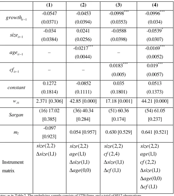
The relationship between cash flow and firm growth differs widely between firm size and firm age. Tables 3 and 4 report GMM-sys results when we split the sample by exogenous criteria of size. Pooled OLS results whe n we split the sample by size are in appendix A.2 and A.3. Using the European Union tradition, firms with fewer than 50 employees were considered micro and small firms and the others are medium and large firms. The sensitivity of firm growth to cash flow appears to be much greater in the sample of smaller firms with

less than 50 employees than for medium and large firms with 50 employees or more. Analysing the results by firm size we find much weaker effects from cash flow for medium and large firms. This result is consistent with the idea that small firms which face more financ ing constraints and are more sensitive to the availability of internal finance grow more than the larger ones. Larger firms can finance their growth from internal resources, debt or issuance of equity. By contrast, smaller firms are limited in the extent of their internal earnings. The weaker effects from cash flow for medium and large Portuguese manufacturing firms may be explained by institutional characteristics. There is one institutional feature of the Portuguese financial system that is in sharp contrast to that practised in the US and UK, both of which may impact the extent to which liquidity constraints occur. The institutional difference that may directly impact the relationship between firm size and growth involves the system of firm finance. Portugal can be classified in the “bank-oriented financial system” along with the French-origin OECD countries (Belgium, France, Greece, Italy and Spain). Given the specific characteristics of the Portuguese financial system, based on an undeveloped stock market, compared with not only the US, but to some extent, other large European countries as well, and in keeping with an industrial structure which includes a relatively large number of small and medium sized firms, we may expect small and large firms to have a complex dependence on internal funds. This complexity is reinforced by a concentrated ownership (lack of ownership dispersion) and control (lack of separation between ownership and control) even of large firms, giving its family owners an active interest in the day-to-day operations of the typical firm. Like other Continental European countries, the Portuguese stock market is not an important source of finance and ownership is concentrated among quoted and not-quoted firms.

In relation to Sargan and second-order serial correlation tests we find that the Sargan test is always accepted, with the exception of columns 2 and 3 in Table 3. This confirms the validity of the instrument matrix used. Furthermore, the consistency of the results is confirmed by the acceptance of m₂statistics.

Table 3: GMM - sys results for micro and small firms (< 50 employees) (1) (2) (3) (4) 1 − it growth -0.1088 *** (0.0212) -0.128*** (0.0157) -0.1194*** (0.0174) -0.1295*** (0.018) 1 − it size -0.1046 (0.1165) 0.0349 (0.0238) -0.0824*** (0.0236) -0.0278 (0.0185) 1 − it age – -0.0401 *** (0.0072) – -0.0327*** (0.0055) 1 − it cf – – 0.0391 *** (0.0041) 0.0353*** (0.0041) constant 0.2655 (0.3028) -0.0006 (0.0459) -0.1494** (0.0656) -0.180*** (0.0338) JS w 75.28 [0.000] 201.7 [0.000] 140.9 [0.000] 267.2 [0.000] Sargan (16) 12.57 [0.704] (36) 68.87 [0.001] (34) 50.42 [0.035] (54) 61.40 [0.228] m2 0.896 [0.370] 0.660 [0.509] 0.856 [0.392] 0.699 [0.484] Instrument matrix ) 1 , 1 ( ) 2 , 2 ( size size ∆ ) 0 , 0 ( ) 1 , 1 ( ) 1 , 1 ( ) 2 , 2 ( age size age size ∆ ∆ ) 1 , 1 ( ) 1 , 1 ( ) 2 , 2 ( ) 2 , 2 ( cf size cf size ∆ ∆ ) 1 , 1 ( ) 0 , 0 ( ) 1 , 1 ( ) 2 , 2 ( ) 1 , 1 ( ) 2 , 2 ( cf age size cf age size ∆ ∆ ∆

Table 4: GMM - sys results for medium and large firms (≥50 employees) (1) (2) (3) (4) 1 − it growth -0.0547 (0.0371) -0.0453 (0.0394) -0.0998*** (0.0353) -0.0996*** (0.034) 1 − it size -0.034 (0.0384) 0.0241 (0.0256) -0.0588 (0.0398) -0.0539* (0.0307) 1 − it age – -0.0217 *** (0.0044) – -0.0169*** (0.0052) 1 − it cf – – 0.0183 *** (0.005) 0.019*** (0.0057) constant 0.1272 (0.1814) -0.0852 (0.1111) 0.035 (0.1801) 0.0513 (0.1373) JS w 2.371 [0.306] 42.85 [0.000] 17.18 [0.001] 44.21 [0.000] Sargan (16) 17.02 [0.385] (36) 40.34 [0.284] (51) 60.36 [0.174] (54) 61.05 [0.237] m2 -0.097 [0.923] 0.054 [0.957] 0.630 [0.529] 0.641 [0.521] Instrument matrix ) 1 , 1 ( ) 2 , 2 ( size size ∆ ) 0 , 0 ( ) 1 , 1 ( ) 1 , 1 ( ) 2 , 2 ( age size age size ∆ ∆ ) 1 , 1 ( ) 1 , 1 ( ) 4 , 2 ( ) 2 , 2 ( cf size cf size ∆ ∆ ) 1 , 1 ( ) 0 , 0 ( ) 1 , 1 ( ) 2 , 2 ( ) 1 , 1 ( ) 2 , 2 ( cf age size cf age size ∆ ∆ ∆

Notes: as in Table 2. The underlying sample consists of 1779 firms and a total of 8512 observations.

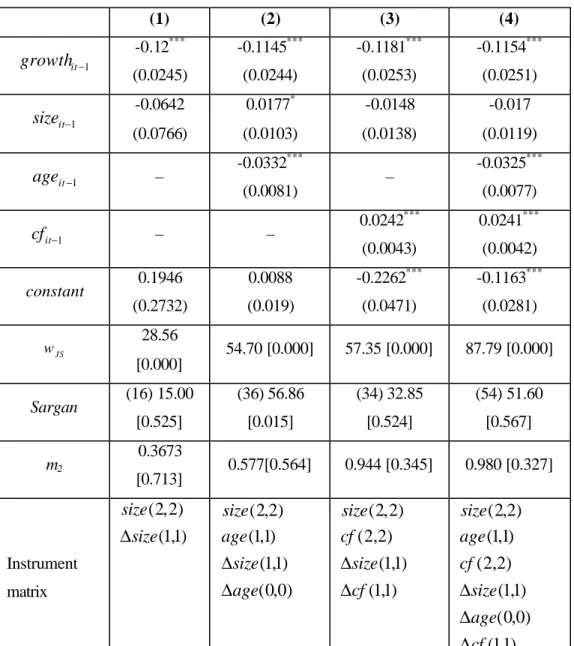
Finally, Tables 5 and 6 report the GMM-sys results when we split the sample by firm age. In particular, Table 5 reports the results for young firms aged 10 years or less, whilst Table 6 shows the same results for old firms aged over 10. Pooled OLS results for young and old firms are given in appendices A.4 and A.5 respectively. As before, analysing Table 5 we find that the cash flow coefficient is again positive and statistically significant at 1% level, 0.0449 and 0.0422 in columns 3 and 4, respectively. But this estimated coefficient is higher for the sample of young firms than for the whole sample. By comparing these results with those reported in Table 6 for mature firms, we conclude that the estimated coefficient for cash flow is lower for older firms. In brief, the variable cash flow appears to play a much more important role in the samples of small and young firms than in the other samples. Regarding

the Sargan and second order serial correlation tests, we find that the Sargan test is always accepted, with the exceptions of column 3 in Table 5 and column 2 in Table 6. The second-order serial correlations test is never rejected. This confirms the consistency of the results.

Table 5: GMM - sys results for young firms (≤ 10 years old)

(1) (2) (3) (4) 1 − it growth -0.1073 *** (0.0237) -0.1227*** (0.0181) -0.1325*** (0.0184) -0.1389*** (0.0191) 1 − it size -0.0913 (0.1319) 0.0245 (0.0185) -0.074*** (0.0213) -0.0398** (0.0186) 1 − it age – -0.0439 *** (0.0091) – -0.0323*** (0.0083) 1 − it cf – – 0.0449 *** (0.0053) 0.0422*** (0.0053) constant 0.2691 (0.3772) 0.0146 (0.0416) -0.2092*** (0.0664) -0.2211*** (0.0448) JS w 52.40 [0.000] 73.83 [0.000] 111.9 [0.000] 139.1 [0.000] Sargan (16) 13.99 [0.599] (45) 52.88 [0.196] (34) 46.80 [0.071] (54) 52.72 [0.524] m2 0.4145 [0.678] 0.3345 [0.738] 0.1709 [0.864] 0.1273 [0.899] Instrument matrix ) 1 , 1 ( ) 2 , 2 ( size size ∆ ) 0 , 0 ( ) 1 , 1 ( ) 2 , 1 ( ) 2 , 2 ( age size age size ∆ ∆ ) 1 , 1 ( ) 1 , 1 ( ) 2 , 2 ( ) 2 , 2 ( cf size cf size ∆ ∆ ) 1 , 1 ( ) 0 , 0 ( ) 1 , 1 ( ) 2 , 2 ( ) 1 , 1 ( ) 2 , 2 ( cf age size cf age size ∆ ∆ ∆

Table 6: GMM - sys results for old firms (> 10 years old) (1) (2) (3) (4) 1 − it growth -0.12 *** (0.0245) -0.1145*** (0.0244) -0.1181*** (0.0253) -0.1154*** (0.0251) 1 − it size -0.0642 (0.0766) 0.0177* (0.0103) -0.0148 (0.0138) -0.017 (0.0119) 1 − it age – -0.0332 *** (0.0081) – -0.0325*** (0.0077) 1 − it cf – – 0.0242 *** (0.0043) 0.0241*** (0.0042) constant 0.1946 (0.2732) 0.0088 (0.019) -0.2262*** (0.0471) -0.1163*** (0.0281) JS w 28.56 [0.000] 54.70 [0.000] 57.35 [0.000] 87.79 [0.000] Sargan (16) 15.00 [0.525] (36) 56.86 [0.015] (34) 32.85 [0.524] (54) 51.60 [0.567] m2 0.3673 [0.713] 0.577[0.564] 0.944 [0.345] 0.980 [0.327] Instrument matrix ) 1 , 1 ( ) 2 , 2 ( size size ∆ ) 0 , 0 ( ) 1 , 1 ( ) 1 , 1 ( ) 2 , 2 ( age size age size ∆ ∆ ) 1 , 1 ( ) 1 , 1 ( ) 2 , 2 ( ) 2 , 2 ( cf size cf size ∆ ∆ ) 1 , 1 ( ) 0 , 0 ( ) 1 , 1 ( ) 2 , 2 ( ) 1 , 1 ( ) 2 , 2 ( cf age size cf age size ∆ ∆ ∆

Notes: as in Table 2. The underlying sample consists of 3858 firms and a total of 17957 observations.

6. Conclusions and implications

Taking unbalanced panel data on Portuguese manufacturing (surviving) firms over the period 1990-2001 to estimate a dynamic panel data model of firm growth that includes serial correlation and financing constraints using the pooled OLS and GMM-sys techniques, the purpose of this paper is to analyse whether liquidity constraints faced by business firms affect firm growth. Our overall results suggest that the growth of Portuguese manufacturing firms is finance constrained. However, when we split our sample by firm size and firm age we find that the smaller and young firms’ growth is more limited in terms of the cash flow available,

which signals greater financing constraints for these firms. Capital constraints are more likely to affect the growth of smaller and younger firms. The severity of financial constraints may be related to financial markets. Portuguese capital markets are still relatively undeveloped and recourse to equity is limited to a reduced number of firms. Thus, companies typically rely almost exclusively on banks for external finance. However, for smaller and young firms the dependence on internal earnings is stronger.

Since small firms account for a large share of employment growth and since many small firms engage in highly innovative activities, one might argue that small- firm activity generates benefits that contribute to the long-run growth of the economy. One might argue for policy recommendations favouring small firms. The policy makers should strongly consider the implementation of programs to promote the birth, growth and innovation activities of small firms. In addition, policy makers should take measures to favour development of the financial market: stimulating market transparency; improving access to information; to stimulate to support, and to develop venture capital.

Appendix

Table A.1: Pooled OLS results for whole sample

(1) (2) (3) (4) 1 − it growth -0.1212 *** (0.0118) -0.1328*** (0.0118) -0.1266*** (0.0124) -0.1381*** (0.0124) 1 − it size -0.0111 *** (0.001) -0.0058*** (0.0011) -0.049*** (0.0022) -0.0436*** (0.0022) 1 − it age – -0.0266 *** (0.0019) – -0.0257*** (0.002) 1 − it cf – – 0.0312 *** (0.0014) 0.031*** (0.0014) constant 0.0213 *** (0.0076) 0.0718*** (0.0086) -0.1652*** (0.0112) -0.1146*** (0.0118) JS w 235.3 [0.000] 381.7 [0.000] 592.1[0.000] 739.4 [0.000] m2 -0.8295 [0.407] -1.571 [0.116] -0.592 [0.554] -1.266 [0.205] Notes: All estimates include a full set of time dummies. The null hypothesis that each coefficient is equal to zero is tested using robust standard errors. Asymptotic standard errors robust to general cross-section and time-series heteroskedasticity are reported in parenthesis. WJS is the Wald statistic of joint significance of the independent variables (excluding time dummies and the constant term). m2 is a test of the null hypothesis of no second-order serial correlation. P-values in square brackets. The underlying sample consists of 7653 firms and a total of 34482 observations.

Table A.2: Pooled OLS results for micro and small firms (< 50 employees) (1) (2) (3) (4) 1 − it growth -0.1373 *** (0.0125) -0.149*** (0.0125) -0.1357*** (0.0135) -0.1466*** (0.0136) 1 − it size -0.017 *** (0.002) -0.0116*** (0.002) -0.0597*** (0.0033) -0.0537*** (0.0034) 1 − it age – -0.0295 *** (0.0024) – -0.0265*** (0.0025) 1 − it cf – – 0.0361 *** (0.0017) 0.0354*** (0.0017) constant 0.0393 *** (0.0105) 0.0954*** (0.0114) -0.1805*** (0.0145) -0.125*** (0.0153) JS w 221.0 [0.000] 346.2 [0.000] 524.4 [0.000] 623.9 [0.000] m2 -1.210 [0.226] -1.918 [0.055] -1.043 [0.297] -1.645 [0.100] Notes: as in Table A.1. The underlying sample consists of 5874 firms and a total of 25970 observations.

Table A.3: Pooled OLS results for medium and large firms (≥ 50 employees)

(1) (2) (3) (4) 1 − it growth 0.0079 (0.0343) -0.0023 (0.0344) -0.037 (0.0325) -0.05 (0.0322) 1 − it size -0.0071 *** (0.0025) -0.0045* (0.0025) -0.0284*** (0.0035) -0.0267*** (0.0034) 1 − it age – -0.0172 *** (0.0032) – -0.02*** (0.0031) 1 − it cf – – 0.0164 *** (0.0017) 0.0173*** (0.0017) constant -0.0004 (0.0146) 0.0375** (0.0162) -0.0915*** (0.0177) -0.0524*** (0.0186) JS w 8.606 [0.014] 39.34 [0.000] 105.5 [0.000] 153.5 [0.000] m2 2.184 [0.029] 1.833 [0.067] 3.664 [0.000] 3.084 [0.002] Notes: as in Table A.1. The underlying sample consists of 1779 firms and a total of 8512 observations.

Table A.4: Pooled OLS results for young firms (≤ 10 years old) (1) (2) (3) (4) 1 − it growth -0.1274 *** (0.0146) -0.1335*** (0.0146) -0.1306*** (0.0151) -0.1354*** (0.0151) 1 − it size -0.0126 *** (0.0018) -0.0109*** (0.0018) -0.053*** (0.0034) -0.051*** (0.0034) 1 − it age – -0.0341 *** (0.005) – -0.026*** (0.0052) 1 − it cf – – 0.0358 *** (0.0022) 0.0352*** (0.0022) constant 0.0474 *** (0.0132) 0.1032*** (0.0157) -0.1736*** (0.0196) -0.1263*** (0.0222) JS w 135.2 [0.000] 168.8 [0.000] 306.8 [0.000] 331.9 [0.000] m2 -0.731 [0.465] -1.023 [0.306] -0.204 [0.839] -0.431 [0.667] Notes: as in Table A.1. The underlying sample consists of 3795 firms and a total of 16525 observations.

Table A.5: Pooled OLS results for old firms (> 10 years old)

(1) (2) (3) (4) 1 − it growth -0.128 *** (0.0198) -0.1311*** (0.0197) -0.1385*** (0.0213) -0.1419*** (0.0213) 1 − it size -0.0038 *** (0.0013) -0.0022* (0.0013) -0.0372*** (0.0027) -0.0357*** (0.0028) 1 − it age – -0.0191 *** (0.004) – -0.0208*** (0.0039) 1 − it cf – – 0.0261 *** (0.0016) 0.0264*** (0.0016) constant -0.0213 ** (0.0087) 0.0324** (0.0144) -0.171*** (0.0127) -0.1146*** (0.0168) JS w 57.67 [0.000] 79.87 [0.000] 288.0 [0.000] 328.2 [0.000] m2 -1.056 [0.291] -1.165 [0.244] -1.119 [0.263] -1.226 [0.220] Notes: as in Table A.1. The underlying sample consists of 3858 firms and a total of 17957 observations.

References

ACS, Zoltan and AUDRETSCH, David (1990) “Innovations and small firms”, Cambridge MA: The MIT Press.

ARELLANO, M. and BOND, S. (1991) “Some tests of specification for panel data: Monte Carlo evidence and an application to employment equations”, Review of Economic Studies, 58, 277-297.

AUDRETSCH, D., and ELSTON, J. (2002) “Does firm size matter? Evidence on the impact of liquidity constraints on firm investment behaviour in Germany”, International Journal of Industrial Organization, 20(1), 1-17.

BECCHETTI, L. and G. TROVATO (2002) “The Determinations of Growth for Small and Medium Sized Firms. The Role of Availability of External Finance”, Small Business Economics,19, 291-306.

BINKS, M. and ENNEW, C. (1996) “Growing firms and the credit constraint”, Small

Business Economics, 8, 17-25.

BINKS, M. and ENNEW, T. (1996) “Financing small firms” In P. Burns and J. Dewhurst, (eds), Small Business and Entrepreneurship, 2nd Ed., Macmillan.

BLUNDELL, R. and BOND, S. (1998) “Initial conditions and moment restrictions in dynamic panel data models”, Journal of Econometrics, 87, 115-143.

BOND, S. and MEGHIR, C. (1994) “Dynamic investment models and the firms financial policy”, Review of Economic Studies, 61, 197-222.

BOND, S., ELSTON, J., MAIRESSE, J., and MULKAY, B. (2003) “Financial factors and investment in Belgium, France, Germany, and the UK: a comparison using company panel data”, Review of Economics and Statistics, 85(1), 153-165.

BOUGHEAS, S., GÖRG, H. and STROBL, E. (2003) “Is R&D Financially Constrained? Theory and Evidence from Irish Manufacturing”, Review of Industrial Organization, 22, 159–174.

BROCK, W. and EVANS, D. (1989) “Small business economics”, Small Business

Economics, 1, 7-20.

BUDINA, N., GARRETSEN, H., and JONG, E. (2000) “Liquidity constraints and investment in transition economies: the case of Bulgaria”, Economics of Transition, 8, 453-475.

BUTTERS, J. and LINTNER, J. (1945) “Effect of federal taxes on growing enterprises”, Boston, Harvard University.

CABRAL, L. and MATA, J. (2003) “On the Evolution of the Firm Size Distribution: Facts and Theory”, American Economic Review, 93(4), 1075-1090.

CARPENTER, Robert and PETERSEN, Bruce (2002) “Is the growth of small firms constrained by internal finance?”, Review of Economics and Statistics, 84(2), 298-309. CAVES, R. (1998) “Industrial organization and new findings on the turnover and mobility of

firms”, Journal of Economic Literature, 36, 1947-1982.

COOLEY, T. and QUADRINI, V. (2001) “Financial Markets and Firm Dynamics”,

American Economic Review, 91(5), 1286-1310.

CRESSY, R. (1996) “Are business start- ups debt rationed?”, Economic Journal, 106(438), 1253-1270.

DAS, S. (1995) “Size, age and firm growth in an infant industry: the computer hardware industry in India”, International Journal of Industrial Organization, 13, 111-126. DAVIS, S., HALTIWANGER, J. and SCHUH, S. (1996) “Job creation and destruction”,

Cambridge, MIT Press.

DEMIRGUC-KUNT, A. and MAKSIMOVIC, V. (1998) “Law, finance, and firm growth,”

Journal of Finance, 53, 2107-2137.

DESAI, M., GOMPERS, P., and LERNER, J. (2003) “Institutions, capital constraints and entrepreneurial firm dynamics: evidence from Europe”, NBER WP series nº 10165. DEVEREUX, M. and SCHIANTARELLI, F. (1990) “Investment, financial factors and cash

flow: evidence from UK panel data” in R. Glenn Hubbard (editor), Asymmetric Information, Corporate Finance and Investment, Chicago, University of Chicago Press. DOORNIK, J., ARELLANO, M. and BOND, S. (2002) “Panel data estimation using DPD

for OX” http://www.nuff.ox.ac.uk/Users/ Doornik/.

DUNNE, T. and HUGHES, A. (1994) “Age, size, growth and survival: UK companies in the 1980s”, The Journal of Industrial Economics, 42, 115-140.

DUNNE, T., ROBERTS, M, and SAMUELSON, L. (1989) “The growth and failure of US manufacturing plants”, Quarterly Journal of Economics, 104, 671-698.

ELSTON, J. (1993) “Firm ownership structure and investment theory and evidence from German panel data”, Wissenschaftszentrum Berlin (WZB) DP FS IV 93-28.

ELSTON, J. (2002) “An Examination of the Relationship Between Firm Size, Growth, and Liquidity in the Neuer Market”, Discussion Paper 15/02, Economic Research Center of the Deutsche Bundesbank.

Economy, 95 (4), 657-674.

EVANS, D. (1987b) “The relationship between firm growth, size and age: estimates for 100 manufacturing industries”, Journal of Industrial Economics, 35(4), 567-581.

EVANS, D. and JOVANOVIC, Boyan (1989) “An Estimated Model of Entrepreneurial Choice under Liquidity Constraints” Journal of Political Economy, 97(4), 808-827. FAGIOLO, G. and A. LUZZI (2004) “Do Liquidity Constraints Matter in Explaining Firm

Size and Growth? Some Evidence from the Italian Manufacturing Industry”, Laboratory of Economics and Management Working Papers 2004/08, Sant’Anna School of Advanced Studies, Pisa.

FARINAS, J. and MORENO, L. (2000) “Firms’ growth, size and age: a nonparametric approach”, Review of Industrial Organization, 17, 249-265.

FAZZARI, S., HUBBARD, G. and PETERSEN, B. (1988) “Financing constraints and corporate investment”, Brookings Papers on Economic Activity, 19, 141-195.

FAZZARI, S., HUBBARD, G. and PETERSEN, B. (2000). “Investment-cash flow sensitivities are useful: a comment on Kaplan and Zingales”, Quarterly Journal of Economics, 115(2), 695-713.

FOTOPOULOS, G., and LOURI, H. (2004) “Firm growth and FDI: are multinationals stimulating local industrial development?”, Journal of Industry, Competition and Trade, 4(3), 163-189.

GEROSKI, P. (1995) “What do we know about entry?”, International Journal of Industrial Organization, 13, 421- 440.

GIBRAT, Robert (1931) “Les Inegalites Economiques”, Paris: Recueil Sirey.

GODDARD, J., MCKILLOP, D. and WILSON, J. (2002) “Credit union size and growth: tests of the Law of Proportionate Effect”, Journal of Banking and Finance, 22, 2327-2356.

GODDARD, J., WILSON, J. and BLANDON, P. (2002) “Panel Tests of Gibrat’s Law for Japanese Manufacturing”, International Journal of Industrial Organization, 20, 415-433.

HALL, B. (1987) “The relationship between firm size and firm growth in the US manufacturing sector”, Journal of Industrial Economics, 35(4), 583-605.

HALL, B. (1992) “Investment and Research and Development at the Firm Level: Does de Source of Financing Matter?”, NBER WP 4096.

Journal of Economics and Management Strategy, 3, 521-543.

HARHOFF, D. (1998) “Are there financing constraints for R&D and investment in German manufacturing firms?”, Annales d’Économie et de Statistique, 49/50, 421-456.

HART, P. E. and OULTON, N. (1996) “Growth and size of firms”, The Economic Journal, 106, 1242-1252.

HESHMATI, A. (2001) “On the growth of micro and sma ll firms: evidence from Sweden”,

Small Business Economics, 17, 213-228.

HOLTZ- EAKIN, D., JOULFAIAN, D. and ROSEN, H. (1994) “Sticking it out: entrepreneurial survival and liquidity constraints”, Journal of Political Economy, 102(1), 53-75.

HOSHI, T., KAYSHAP, A. and SCHARFSTEIN, D. (1991), “Corporate structure, liquidity, and investment: evidence from Japanese industrial groups”, Quarterly Journal of Economics, 106, 33-60.

HUTCHINSON, J. and XAVIER, A. (2004) “Comparing the impact of credit constraints on the growth of SME’s in a transition country with an established market economy”, LICOS Centre for Transition Economics Discussion Papers Series, Katholieke Universiteit Leuven, DP150/2004.

JOVANOVIC, B. (1982) “Selection and the evolution of industry”, Econometrica, 50(3), 649-670.

KAPLAN, S. and ZINGALES, L. (1997) “Do investment-cash flow sensitivities provide useful measures of financing constraints?”, Quarterly Journal of Economics, 112(1), 169-215.

KAPLAN, S. and ZINGALES, L. (2000) “Investment- cash flow sensitivities provide useful measures of financing constraints”, Quarterly Journal of Economics, 115(1), 707-712. KLAPPER, L., SARRIA-ALLENDE, V., and SULLA, V. (2002) “Small and medium size

enterprise financing in Eastern Europe”, World Bank Policy Research WP 2933.

KLETTE, J. and GRILICHES, Z. (2000) “Empirical patterns of firm growth and R&D investment: a quality leader model interpretation”, Economic Journal, 110, 363-387. KONINGS, J., RIZOV, M., and VANDENBUSSCHE, H. (2003) “Investment and credit

constraints in transition economies: Micro evidence from Poland, the Czech Republic, Bulgaria and Romania”, Economics Letters, 78(2), 253-258.

KUMAR, K., RAJAN, R. and ZINGALES, L. (1999) “What determines firm size?”, National Bureau of Economic Research, WP 7208.

KUMAR, M. S. (1985) “Growth, acquisition activity and firm size: evidence from the United Kingdom”, Journal of Industrial Economics, 33(3), 327-338.

LANG, L., OFEK, E. and STULZ, R. (1996) “Leverage, investment, and firm growth”,

Journal of Financial Economics, 40, 3-29.

NURMI, S. (2003) “Plant size, age and growth in Finnish manufacturing”, Institute of Fiscal studies, London. http://cemmap.ifs.org.uk/docs/eea_nurmi.pdf.

PAKES, A. and ERICSON, R. (1998) “Empirical implications of alternative models of firm dynamics”, Journal of Economic Theory, 79, 1-45.

PISSARIDES, F. (1998) “Is the lack of funds the main obstacle to growth? The EBRD’s experienced with small and medium sized business in Central and Eastern Europe”, EBRD WP 33.

SCHERER, Fredric M., and ROSS, David (1990) “Industrial Market Structure and Economic Performance”, 3rd ed., Boston: Houghton Mifflin Company.

SCHIANTARELLI, F. (1996) “Financial constraints and inve stment: methodological issues and international evidence”, Oxford Review of Economic Policy, 12(2), 70-89.

SUTTON, John (1997) “Gibrat’s Legacy”, Journal of Economic Literature, 35(1), 20-49. TSCHOEGL, A. (1983) “Size, growth and transnationality among the world’s largest banks”,

Journal of Business, 56, 187-201.

VARIYAM, J. and KRAYBILL, D. (1992) “Empirical evidence on determinants of firm growth”, Economic Letters, 38, 31-36.

WAGENVOORT, R. (2003) “Are finance constraints hindering the growth of SME’s in Europe?”, European Investment Bank Paper, 8(2).

XU, B. (1998) “A re-estimation of the Evans-Jovanovic entrepreneurial choice model”,

Estudos do GEMF

ESTUDOS DO G.E.M.F.

(Available on-line at http://gemf.fe.uc.pt)

2005-07 _{Firm Growth and Liquidity Constraints: A Dynamic Analysis}

- Blandina Oliveira & Adelino Fortunato

2005-06 _{The Effect of Works Councils on Employment Change}

- John T. Addison & Paulino Teixeira

2005-05 _{Le Rôle de la Consommation Publique dans la Croissance: le cas de l'Union Européenne}

- João Sousa Andrade, Maria Adelaide Silva Duarte & Claude Berthomieu 2005-04 _{The Dynamics of the Growth of Firms: Evidence from the Services Sector}

- Blandina Oliveira & Adelino Fortunato

2005-03 _{The Determinants of Firm Performance: Unions, Works Councils, and Employee}

Involvement/High Performance Work Practices

- John T. Addison

2005-02 _{Has the Stability and Growth Pact stabilised? Evidence from a panel of 12 European}

countries and some implications for the reform of the Pact

- Carlos Fonseca Marinheiro

2005-01 _{Sustainability of Portuguese Fiscal Policy in Historical Perspective}

- Carlos Fonseca Marinheiro

2004-03 _{Human capital, mechanisms of technological diffusion and the role of technological shocks}

in the speed of diffusion. Evidence from a panel of Mediterranean countries

- Maria Adelaide Duarte & Marta Simões

2004-02 _{What Have We Learned About The Employment Effects of Severance Pay? Further}

Iterations of Lazear et al.

- John T. Addison & Paulino Teixeira

2004-01 _{How the Gold Standard Functioned in Portugal: an analysis of some macroeconomic aspects} - António Portugal Duarte & João Sousa Andrade

2003-07 _{Testing Gibrat’s Law: Empirical Evidence from a Panel of Portuguese Manufacturing Firms} - Blandina Oliveira & Adelino Fortunato

2003-06 _{Régimes Monétaires et Théorie Quantitative du Produit Nominal au Portugal (1854-1998)} - João Sousa Andrade

2003-05 _{Causas do Atraso na Estabilização da Inflação: Abordagem Teórica e Empírica} - Vítor Castro

2003-04 _{The Effects of Households’ and Firms’ Borrowing Constraints on Economic Growth} - Maria da Conceição Costa Pereira

2003-03 _{Second Order Filter Distribution Approximations for Financial Time Series with Extreme}

Outliers

- J. Q. Smith & António A. F. Santos

2003-02 _{Output Smoothing in EMU and OECD: Can We Forego Government Contribution? A risk}

sharing approach

- Carlos Fonseca Marinheiro

2003-01 _{Um modelo VAR para uma Avaliação Macroeconómica de Efeitos da Integração Europeia}

da Economia Portuguesa