Manning Friction in Steep Open-channel Flow

Seventh International Conference on Computational Fluid Dynamics (ICCFD7), Big Island, Hawaii, July 9-13, 2012

ICCFD7-2012-3303

Manning Friction in Steep Open-channel Flow

Corresponding author: [email protected]

*Department of Civil Engineering and Applied Mechanics, McGill University, Canada Abstract: The Manning friction coefficient as a one-dimensional (1D) open-channel flow parameter is determined from a series of two-dimensional (2D) simulations of the flow on steep slopes using a computational hydraulic solver derived from a minimal intervention strategy (MIS2D). Computations are also conducted for the oblique dam-break waves to evaluate the performance of MIS2D. The results are compared with exact solution and the simulations obtained by a commercial three-dimensional (3D) simulation model (FLOW-3D).

Keywords: Manning Friction, Open-channel Flow, Computational Hydraulics, Flux Limiter, Minimum Intervention Strategy, MIS2D, FLOW-3D.

1 Introduction

Hydraulic engineers are increasingly dependent on computer simulations which can be conducted using either a one-dimensional (1D), a two-dimensional (2D) or a three-dimensional (3D) model. The 1D computational hydraulic model such as HEC-RAS has been used in river flow simulations due to its ease of implementation and the acceptance by the engineering profession [2]. However, with the growth of the technology such as LIDAR, accurate topographic information can be resolved with precision and used as input for 2D computer simulations. In flood-plain flow and lake circulation simulations, the 2D model is a much better representation of the reality. Given the large horizontal length scale of the flow in rivers and lakes, the 2D model appears to be adequate despite the availability of commercial 3D simulation models. The 2D model based on the shallow-water approximation is computationally more economical compared with the 3D model which requires the numerical solution of the full Navier-Stokes equations. The selection of a proper model to suit a particular problem nevertheless depends on the modeler’s knowledge and experience as well as the nature of the problem.

A series of 2D computer simulations is conducted in steep open-channel flow using a minimal intervention strategy (MIS) to manage the spurious oscillations [9, 13]. This MIS2D model is trans-critical. The MIS2D solver is equally accurate for sub-critical and super-critical open-channel flow. The performance of the MIS2D is evaluated by first conducting a dam-break wave simulation. The results are compared with the exact solution and the simulations obtained by commercial software known as FLOW-3D. In the subsequent simulations of steep open channel flow, the performance of the MIS2D is evaluated using the Manning friction coefficient as a performance indicator.

2 Trans-critical Solver MIS2D

The development of the trans-critical solver for 2D numerical simulation of the shallow open-channel flow is based on finite-volume formulation using a staggered grid. As shown in Fig. 1a, the center of

the finite volume for the continuity equation is defined at the h node. For the x- and y-momentum equations, the center is defined at the qx-node and the qy-node as shown in Fig. 1b and 1c,

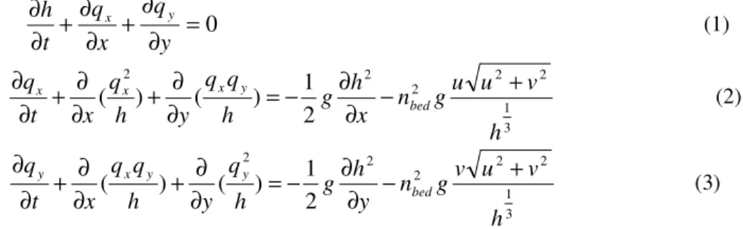
respectively. The finite-difference equations in the limit as ∆x and ∆y approach zero are the partial differential equations: =0 ∂ ∂ + ∂ ∂ + ∂ ∂ y q x q t h x y ₍₁₎ 3 1 2 2 2 2 2 2 1 ) ( ) ( h v u u g n x h g h q q y h q x t q bed y x x x ₋ + ∂ ∂ − = ∂ ∂ + ∂ ∂ + ∂ ∂ (2) 3 1 2 2 2 2 2 2 1 ) ( ) ( h v u v g n y h g h q y h q q x t q bed y y x y + − ∂ ∂ − = ∂ ∂ + ∂ ∂ + ∂ ∂ (3)

where h = total depth, (qx, qy) = x- and y-components of the depth-averaged flow, g = gravity, (u, v) =

x- and y-components of the flow velocity, and nbed = Manning friction coefficient for the channel bed.

These shallow-water equations for open-channel flow are not hyperbolic equations in general. To control the spurious numerical oscillations, most flux limiting solution methods are developed by treating the shallow equations to be hyperbolic [7, 8, 10, 12].

(

q

)

h

(

q

)

∆

y

∆

x

q

−

volume

q

−

volume

(

q

)

(

q

)

( )

qˆ

( )

,

h

ˆ

q

ˆ

( )

,

hˆ

qˆ

( )

qˆ

( )

q

ˆ

( )

,

q

ˆ

( )

,

q

ˆ

( )

q

ˆ

hˆ

h

ˆ

(a)

(b)

(c)

Figure 1: The nodes for hi,j, (qx)i,j, and(qy)i,j and the finite control volumes defined by the nodes.

The hyperbolic solvers are effective in capturing the discontinuity of the shock waves. However, they are not efficient and need corrections if used for subcritical flow simulations. The recent development of a non-hyperbolic flow solver by Pinilla et al. [9] and Wang et al. [13] has opened up the opportunity to the solutions of many previously intractable hydraulic engineering problems in open-channel flow. This non-hyperbolic flow solver uses the classical method of consistent transport. The solver resolves the flow discontinuities in shallow water using a minimal intervention strategy (MIS). To control the numerical oscillations, flux limiter is applied only to qx as the qx is updated using the x

numerical integration over time is carried out using a fourth-order Runge-Kutta procedure. This two-dimensional trans-critical solver based on the minimal intervention strategy will be referred as the MIS2D. The implementation details of this MIS2D are explained in Pinilla et al. [9].

3 Oblique Dam-break Waves by MIS2D

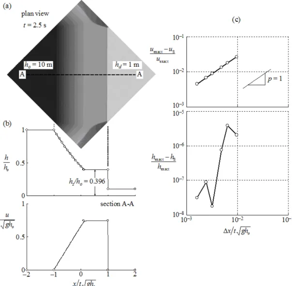
The first simulation example by the MIS2D model is the oblique dam-break waves. The waves are produced in a 100 m × 100 m square basin by the sudden removal of a dam. The initial water depths at time t = 0 are ho = 10 m and hd = 1 m separated by a dam located in the diagonal direction across

the basin. Figure 2a shows the plan view of the waves at time t = 2.5 s. Figure 2b shows the depth and velocity profiles of the waves along the cross section A-A at this time obtained by the MIS2D using the MINMOD flux limiter and using a grid size of ∆x = ∆y = 0.5 m.

Figure 2: Oblique dam-break waves at time t = 2.5 s; (a) plan view, (b) depth and velocity profiles along the cross-section A-A, (c) diminishing error as the MIS2D simulation converges to the exact solution. Circle symbol denotes the exact solution of Stoker [11].

minimally to manage the spurious numerical oscillations. The MIS2D simulation profiles with ∆x =

∆y = 0.5 m are nearly identical to the exact solution obtained by Stoker [11] using the method of characteristic. At time t = 2.5, the wave height is hs/ho = 0.396 and the velocity is us/ gh=0.741

according to the exact solution. Figure 2c shows the convergence of the MIS2D simulation toward the exact solution as the grid is refined. The order of the convergence for velocity us is p ≈ 1 using the

procedure for estimating and reporting of uncertainty as recommended by Celik et al. [3]. The integration of the shallow-water equations by the MIS2D model is second-order accuracy in time and space according to Pinilla et al. [9]. However, the convergence of the surge wave velocity to the exact solution is only first-order. This behavior nevertheless is consistent with the recent Godunov’s assessment on the discontinuous solutions of the shallow-water equations [8].

4 Oblique Dam-break Waves by FLOW-3D

The simulation of the same oblique dam-break waves is repeated using a computational fluid dynamic model known as FLOW-3D developed and commercialized by Flow-Science Inc. [5]. The FLOW-3D uses the finite difference method to solve numerically the Navier-Stokes equations. The spurious numerical oscillations are managed by a second order monotonicity preserving method. FLOW-3D also uses the orthogonal staggered mesh. The volume of fluid (VOF) method is employed in the FLOW-3D to resolve the free water surface. It provides an accurate way to advect the fluid interface through a fixed computational grid while keeping the interface sharp and well defined. There are three key elements which must be in place in any CFD tools in order to be called a VOF method. First, there must be a fluid fraction variable F, which tracks the amount of fluid within a given computational cell. Second, an advection algorithm is required to not only advect F, but to keep the interface sharp. Third, free surface boundary conditions must be applied to the interface. Computer calculates the area and volume ratios in each cell and the ratios are integrated into the conservation equations. The value of each dependant variable is associated to each cell and applied at the centre of the cell except the velocity, which is applied on the face of the cell. In order to solve the mass conservation and movement equations, an explicit solution algorithm is used to evaluate the variables associated with velocities in the Navier-Stokes equation for a given time taking into account the initial conditions or variable values at previous time step. Water pressure is evaluated in each cell and iterations are used to advance the solution through a sequence of steps from a starting state to a final, converged state. The cell corresponding to the velocities are then adjusted. The present FLOW-3D simulation uses an isotropic grid with ∆x = ∆y = ∆z; the dimensions of the grid ∆x and ∆y are the same as the 2D simulations using MIS2D.

The FLOW-3D package also has the ability to do 2D simulation when the 3D modeling is not necessary. This 2D model is referred as FLOW-3D Shallow Water Model that is FLOW-3D-SWM. It allows to model large river reaches, coasts and estuaries, and other large domains. It takes a 2D grid in x- and y-direction and the vertical velocity is assumed to be 0. The model assumes all variables can be represented by their depth-averaged values and solves the 2D momentum equations with corrections for variation in depth.

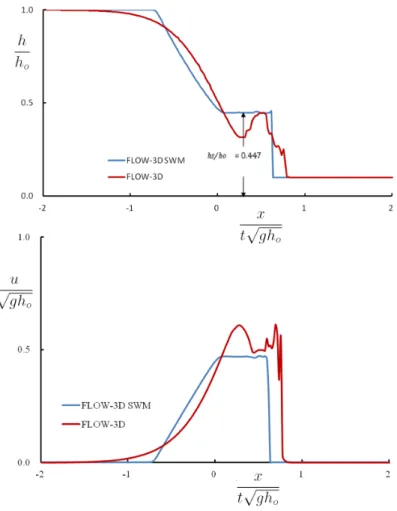
The results of the oblique dam-break waves in a 100-m x 100-m square basin due to sudden removal of the dam are shown in Figs. 3 and 4. The initial depths are ho = 10 m and hd = 1 m. Figure 3 shows

the depth of the waves being color coded by velocity. Figure 4 shows the depth and velocity profiles along the diagonal cross section A-A. These FLOW-3D-SWM and FLOW-3D profiles are to be compared with the exact solution shown in Fig. 2b. At this time t = 2.5 s, the location of surge wave front obtained by FLOW-3D and FLOW-3D-SWM is both behind the supposed location at

0 . 1 /t gh_o =

x and the surge wave height is higher than the exact solution of h/ho = 0.396. The

difference is not large. Since ∆z=0.5m, there are 20 layers on the side where ho = 10 m and only 2

layers on the side where hd = 1m. The large difference in the number of layers at the shock-wave

investigation on the FLOW-3D equations and gird size study will be conducted in future studies to explain the discrepancy between the 2D models and FLOW-3D.

Figure 3: Velocity of the oblique shock wave problem. Left hand side of the figure shows the simulation by FLOW-3D-SWM method while the right hand side of the figure shows the simulation performed by FLOW-3D model.

Figure 4: Comparison of depth and velocity profiles along the diagonal cross section A-A at the time t = 2.5s. Simulations are carried out using the FLOW-3D-SWM and FLOW-3D for the 100-m x 100-m square basin with the grid ∆x = ∆y = ∆z = 0.5 m

5 Macro Resistance to Flow in Steep Open-Channel

The next series of simulations is conducted for open-channel flow on steep slope. As shown in the plan view of Fig. 5, the macro resistance to the open-channel flow is due to an array of blocks. The channel has an initial depth ho = 2 m and block width b = 10 m. Three channel-bottom slopes are

considered at So = 0.005, 0.01 and 0.04. Periodic boundary condition is given at the left and right

boundaries. The effect of bottom friction is eliminated by setting the roughness to zero and the effect of viscosity is eliminated by not activating the turbulence model. Therefore, the gravity component along the slope is the only driving force to cause the water to flow along the slope of the channel. The flow through the periodic arrays of blocks in Fig. 5 is idealized in an attempt to mimic the steep flow in mountain streams. The navigation of water around rocks and boulders in the mountain stream such as the one shown in Fig. 6 is a process distinctively different from the slow flow through large rivers. In steep channels, the flow changes rapidly from subcritical to supercritical at the control sections. The photo of the steep mountain stream in Fig. 6 depicts the process. Significant energy

dissipation occurs in the hydraulic jumps as the supercritical flow returns to its subcritical state. The white waters in the steep river are the demarcation for the return of supercritical flow to its subcritical state. L= 120m b B = 7 0 m b b

(a)

1

2

3

4

Figure 5: Plan view of the open-channel flow through an array of blocks. Simulations are conducted using a periodic boundary condition.

Figure 6: The transition from subcritical to supercritical flow at the control sections and the return to subcritical flow through the hydraulic jumps. The white waters mark the location of the jumps. In the present simulation, such flow resistance is directly determined by the MIS2D, FLOW-3D, and FLOW-3D-SWM models. The simulations begin with a fixed initial depth of 2 m. Driven by the gravity, the flow through the channel first accelerates and then reaches a quasi-steady state. Figures 7, 8, and 9 show the Froude number and depth maps for the three slopes So = 0.005, 0.01 and 0.04

respectively using the three simulation methods with grid size ∆x = ∆y = ∆z = 0.5 m. There are only two fluid layers over the depth of 1 m in the FLOW-3D simulations. It is shown the MIS2D results give more fluctuations in Froude number and water depth while the FLOW-3D simulation results are less turbulent.

Figure 7: Froude number and water depth distribution in a steep open channel on slope So = 0.005.

Top: MIS2D simulation result; Middle: FLOW-3D result; Bottom: FLOW-3D-SWM result.

Figure 8: Froude number and water depth distribution in a steep open channel on slope So = 0.01. Top:

Figure 9: Froude number and water depth distribution in a steep open channel on slope So = 0.04. Top:

MIS2D simulation result; Middle: FLOW-3D result; Bottom: FLOW-3D-SWM result.

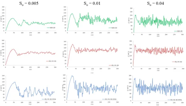
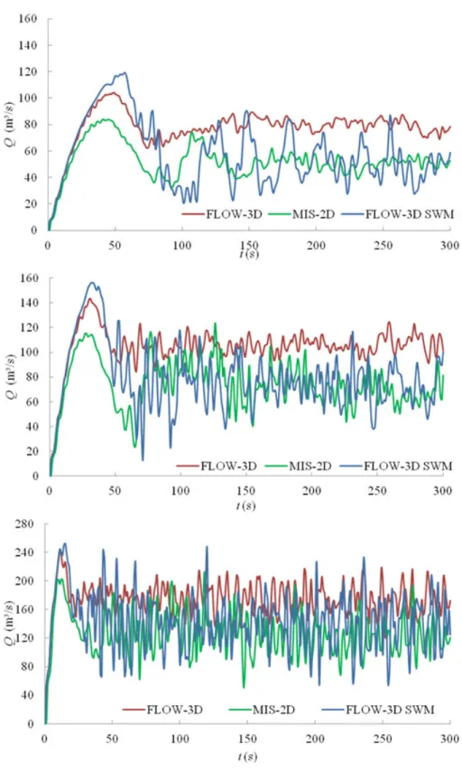
The total discharge Q through the channel is obtained by integration of the velocity over the channel cross section. Figure 10 shows the graphs of the discharge rates Q plotted against the time t for the results obtained on the three channel slopes using MIS-2D, FLOW-3D and FLOW-3D-SWM. Figure 11 compares the discharge rates from three methods in the same graph. It is found all the simulations follow the same trend. The water flow rate Q starts to accelerate with gravity initially and then reaches a quasi-steady rate. Higher slope yields higher discharge. The quasi-steady flow Qqs is

reached when the driven force of gravity is in balance with the resistance to flow by the blocks. The two-dimensional methods MIS-2D and FLOW-3D-SWM give comparable Qqs. However, the three

dimensional method FLOW-3D, gives significant higher quasi-steady flow rate than the two dimensional methods. Moreover, the graphs of the FLOW-3D flow rate show less fluctuation. In the present calculations, the Qqs. is the average of Q over the period from 150 s to 300 s. Table 1

summaries the results for Qqs.. The root-mean-square discharge shows the fluctuation of the flow rate

at each time from the average of the quasi-steady rate and it is computed by the formula below and the results are tabulated in Table 2.

qs t qs Q Q t Q Q 2 300 150 ___ 2 ) ) ( ( '

∑

The root-mean-square discharge is significantly lower for the simulation obtained using the FLOW-3D model. Although the FLOW-FLOW-3D-SWM is a 2D model, its root-mean-square value of the discharge is slightly higher. Higher root-mean-square values apparently are associated with scale of the turbulent motions which can be observed from the images shown in Figs. 7, 8 and 9. The scale and nature of the turbulent motions obtained by the three models are clearly different. The results obtained from the 3D model are more different than the difference between the 2D simulation models.

Slope MIS2D FLOW-3D FLOW-3D-SWM

0.005 51.0 80.4 50.8

0.010 70.4 106.4 73.2

0.040 120.7 174.1 140.3

Table 1: Quasi-steady state flow rate Qqs(m³/s) obtained for the three channel slopes So = 0.005, 0.01

and 0.04 using MIS2D, FLOW-3D and FLOW-3D-SWM models.

Slope MIS2D FLOW-3D FLOW-3D-SWM

0.005 1.1 0.7 3.3

0.010 2.0 0.8 2.4

0.040 2.4 1.4 3.1

Table 2: Root-mean-square discharge 2

'

_____

Q

MIS2D, FLOW-3D and FLOW-3D SWM models.

Figure 10: Variation of flow rate Q (m3/s) with time t (s) for the steep open-channel flow on the slopes So = 0.005, 0.01 and 0.04. Top: MIS2D simulation result; Middle: FLOW-3D result; Bottom:

FLOW-3D-SWM result. The quasi-steady-state statistics are determined from the data obtained over the period of time from 150 s to 300 s.

Figure 11: Variation of flow rate in Q (m3/s) with time t (s) for steep open channel flow obtained by the three models MIS2D, FLOW-3D and FLOW-3D-SWM. Top: So = 0.005; Middle: So = 0.01;

6 Manning Coefficient of Friction

The resistance to flow in open channel is traditionally parameterized using the Manning coefficient of friction nbed. The values of nbed are tabulated in Arcement and Dchneider [1] and Chow [4] .The

selection of an appropriate nbed from the tables however is a matter of intangibles as described by Ven

Te Chow [4]: “To veteran engineers, this means the exercise of sound engineering judgment and experience; for beginners, it can be no more than a guess, and different individuals will obtain different results.” Alternatively, the value of nbed can be determined from in-situ measurements as

described in French [6]. Either of these methods can be problematic.

Given the quasi-steady flow rate Qqs, a macro Manning coefficient nmacro is determined from the

following formula: 2 1 3 2 1 o macro qs AR S n Q = (5)

The macro Manning coefficient nmacro is a catch-all parameter for the overall resistance of the blocks

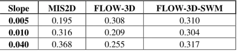
to the flow. The values of nmacrofor different slopes 0.005, 0.01, and 0.04 are given in Table 3. Since

the size of the blocks is large comparing with the channel dimension, the flow of the water is constrained in the areas between the blocks. In this case, the averaged Froude number as shown in Table 4 based on Qqs and hqs is not significantly different among the different channel slopes and

simulation methods.

The specified Manning coefficient nbed is 0. Therefore the resistance to the flow is entirely due to the

form drag produced by the blocks. The macro Manning coefficient is a parameter of the 1D model. The values of this macro coefficient have to be selected subjectively based on judgement in a 1 D model simulation. The macro coefficient shown in Table 3 is more than ten times higher than the typical Manning coefficient of flow on concrete surface of n = 0.014. These results have pointed out the major difficulty of 1 D simulation models. Simulation results obtained by 1D model such as HEC-RAS depend almost entirely on the judicial selection of the Manning coefficient. Incorrect selection of the coefficient could leads to entirely erroneous results.

Slope MIS2D FLOW-3D FLOW-3D-SWM 0.005 0.195 0.308 0.310

0.010 0.316 0.209 0.304

0.040 0.368 0.255 0.317

Table 3: Values of the macro Manning coefficient nmacro for the three channel slopes obtained using

the MIS2D, FLOW-3D and FLOW-3D-SWM models

Slope MIS2D FLOW-3D FLOW-3D-SWM 0.005 0.082 0.130 0.082

0.010 0.113 0.172 0.118

0.040 0.195 0.281 0.226

Table 4: Values of the averaged Froude number based on Qqs and hqs for the three channel slopes

obtained using the MIS2D, FLOW-3D and FLOW-3D-SWM models

The macro Manning coefficient nmacro is also a parameter that can be used as a performance indicator.

This macro coefficient can be seen in the bar graphs show in Fig. 12 to be essentially the same between the simulations obtained by the MIS2D model and FLOW-3D-SWM because both MIS2D

and SWM are 2D models. The root-mean-square discharge obtained by the FLOW-3D-SWM however is higher than the value obtained by the MIS2D.

Figure12: Bar graphs for the quasi-steady flow rate Qqs (top), the Manning friction coefficient

nmacro(middle)and for the root-mean-square discharge

'

_____

Q

7 Conclusion and Future Work

Numerical simulation of dam-break waves using the MIS2D model has produced results in perfect agreement with the exact solution. The spurious numerical oscillations are managed well by the flux limiter using the minimal invention strategy. The two-dimensional FLOW-3D-SWM model has produced not significantly different results. However, the quasi-steady discharges obtained by the dimensional FLOW-3D model are consistently higher. The higher discharges of the three-dimensional model are associated with the corresponding lower macro resistance to flow. The lower macro resistance to flow also correlates clearly with the lower root-mean-square fluctuations of the flow. The resolution to the discontinuities of flow is different between the 2D and 3D simulation models. The 2D produces sharp discontinuities. In reality, however the change from one side to the other side of surge wave is not a discontinuity. It is also not a discontinuity in the 3D simulations. This may explain why 3D turbulence has less fluctuation amplitude and therefore cause less resistance to flow. We are currently carrying additional numerical experiments using finer grid size in order to find the reason for the discrepancy between the two-dimensional and three-dimensional models.

References

1. Arcement, G.J. Jr. and Dchneider, V.R.: Guide for selecting Manning’s roughness coefficients for natural channels and flood plains. U.S. Geological Survey, Water Supply Paper 2339, 38 p., Washington D.C (1989)

2. Brunner, G.W: HEC-RAS River Analysis System User’s Manual Version 4.1.

US Army Corps of Engineers Institute for Water resources Hydrologic Engineering Center, Davis, CA (1989)

3. Celik, I.B., Ghia, U., Roache, P.J., Freitas, C.J., Coleman, H., Raad, P.E.: Procedure for estimation and reporting of uncertainty due to discretization in CFD applications. J. Fluids Engrg.130, 1—4 (2008)

4. Chow, Ven Te: Open-Channel Hydraulics. McGraw-Hill, New York (1959)

5. FLOW Science.: FLOW-3Dv10-User Manual, Flow Science Inc., Santa Fe, NM (2011) 6. French, R. H.: Open-Channel Hydraulics, McGraw-Hill, New York (1984)

7. Godunov, S.K.: A difference scheme for numerical solution of discontinuous solution of hydrodynamic equations, Math. Sbornik 47, 271—306 (1959), translated

US Joint Publ. Res. Service, JPRS 7226, 1969

8. Godunov, S.K.: Remininiscences about numerical schemes. Rapport de

recheerché No. 6666. Theme NUM. Institut National de recherché en informatique et en automatique, p. 25. Le Chesnay Cedex, France (2008)

9. Pinilla, C.E., Bouhairie, S., Tan, L.-W., Chu, V.H. : Minimal intervention to simulations of shallow-water equations. J. Hydro-env. Research, 3(4), 201-207(2010)

10. Roe, P.L.: Approximate Riemann solvers, parameter vectors and difference schemes, J. Comput. Phys., 43, 357-372 (1981)

11. Stoker, J.J. :Water Waves - The mathematical theory with Applications, Wiley Interscience, New York (1957)

12. Toro, E.F.: Riemann Solver and Numerical Methods for Fluid Dynamics. 3rd edn. Springer, New York (2009)

13. Wang, T., Tan, L.-W. and Chu, V.H.: Flood-waves simulation by classical method of consistent transport. Computational Fluid Dynamics 2010, A. Kuzmin ed., Springer (2011)