Credit Rationing, Risk Aversion and Industrial Evolution in Developing Countries

NBER WORKING PAPER SERIES

CREDIT RATIONING, RISK AVERSION AND INDUSTRIAL EVOLUTION IN DEVELOPING COUNTRIES Eric Bond James R. Tybout Hâle Utar Working Paper 14116 http://www.nber.org/papers/w14116

NATIONAL BUREAU OF ECONOMIC RESEARCH 1050 Massachusetts Avenue

Cambridge, MA 02138 June 2008

This paper was funded by NSF grant SES 0095574 and the Pennsylvania State University. The opinions, findings, and conclusions or recommendations expressed herein are those of the authors and do not necessarily reflect the views of the National Science Foundation or the National Bureau of Economic Research. The authors are grateful to Marc Melitz, Chad Syverson, Gregor Matvos and participants in numerous seminars for their comments. The corresponding author is James Tybout.

NBER working papers are circulated for discussion and comment purposes. They have not been peer-reviewed or been subject to the review by the NBER Board of Directors that accompanies official NBER publications.

© 2008 by Eric Bond, James R. Tybout, and Hâle Utar. All rights reserved. Short sections of text, not to exceed two paragraphs, may be quoted without explicit permission provided that full credit, including © notice, is given to the source.

Credit Rationing, Risk Aversion and Industrial Evolution in Developing Countries Eric Bond, James R. Tybout, and Hâle Utar

NBER Working Paper No. 14116 June 2008, Revised August 2010 JEL No. D24,L26,O16

ABSTRACT

Relative to their counterparts in high-income regions, entrepreneurs in developing countries face less efficient financial markets, more volatile macroeconomic conditions, and higher entry costs. This paper develops a dynamic empirical model that links these features of the business environment to cross-firm productivity distributions, entrepreneurs’ welfare, and patterns of industrial evolution. Applied to panel data on Colombian apparel producers, the model yields econometric estimates of a credit market imperfection index, the sunk costs of creating a new business, and a risk aversion index (inter alia). Model-based counterfactual experiments suggest that improved intermediation could dramatically increase the return on assets for entrepreneurial households with modest wealth, and that the gains are particularly large when the macro environment is relatively volatile.

Eric Bond Vanderbilt University Department of Economics VU Station B #351819 2301 Vanderbilt Place Nashville, TN 37235-1819 [email protected] James R. Tybout Department of Economics Penn State University 517 Kern Graduate Building University Park, PA 16802 and NBER [email protected] Hâle Utar University of Colorado Department of Economics 256 UCB Boulder, CO 80309-0256 [email protected]

2 I. Overview

Relative to their counterparts in high-income regions, entrepreneurs in developing countries face less efficient financial markets, more volatile macroeconomic conditions, and higher entry costs.1,2, 3 _{This paper develops a dynamic empirical model that links these features} of the business environment to firm ownership patterns, firm size distributions, productivity distributions, and borrowing patterns.

The model emphasizes several basic effects. First, borrowing constraints force households with modest collateral to either forego profitable entrepreneurial activities or pursue them on an inefficiently small scale. Second, since credit constraints limit households’ ability to smooth their consumption streams, those with relatively less tolerance for risk shy away from business ventures during periods of macro volatility. 4 _{Finally, in combination with substantial} entry costs and a significant spread between borrowing and lending rates, uncertainty about future business conditions creates an incentive for entrepreneurs to continue operating firms that generate sub-market returns. Combined, these effects make firms’ survival and growth less dependent upon their owners’ entrepreneurial ability, and more dependent upon their owners’

1 _{Private credit is scarce (as a share of GDP), spreads between borrowing and lending rates are large, non-bank}

intermediation is relatively unimportant, and equity markets are often almost non-existent. The literature

documenting these patterns of financial development is vast; Beck et al (2000) provide a cross-country data set that reflect the characteristics mentioned here. Levine (2005) surveys the evidence linking these features of financial sectors (among others) to countries’ aggregate growth rates. Djankov et al (2006) empirically link the poor performance of credit markets in developing countries to their lack of legal creditor protections and information-sharing institutions.

2_{Loayza et al (2007) survey the literature on macroeconomic volatility in developing countries and discuss its}

causes and costs. Kaminsky and Reinhardt (1999) document patterns of banking and financial crises in developing countries. Tybout (2000) provides additional references and notes that Latin America and Sub-Saharan Africa stand out among the developing countries as the most volatile, but all developing regions do worse than the industrialized countries.

3 _{Surveying entry regulations in 85 countries, Djankov et al (2002) conclude that ―business entry is extremely}

expensive, especially in the countries outside the top quartile of the income distribution.‖ (p. 25)

4 _{Volatility can also change the types of capital goods that entrepreneurs invest in, as in Lambson (1991) and}

3 wealth and market-wide volatility.

We fit our model to plant-level panel data and macro data from Colombia, obtaining econometric estimates of plant-level profit functions, the sunk cost of creating a new business, and an index of credit market imperfections (inter alia). Then, using our estimated parameters, we simulate industrial evolution patterns under alternative assumptions about credit market imperfections. In particular, we explore the effects of credit market imperfections and volatile macro environments on entry and exit patterns, cross-firm investment patterns, industry-wide productivity distributions, and savings.

The simulations yield a number of findings. First, the credit markets in which small-scale Colombian entrepreneurs operate are subject to severe contract enforcement problems. These problems interact with macro volatility, substantial entry costs, and risk aversion to discourage households with modest wealth from investing in proprietorships—even those with high earnings potential. Second, if enforcement problems were eliminated so that entrepreneurs were less dependent upon self-finance, those with relatively modest wealth but high earnings potential would expand their businesses significantly relative to others. Also, the option value of remaining in business would fall for firms with low earnings rates, and some of these would exit. Combined, these two effects would increase the industry-wide overall rate of return on the wealth portfolios of entrepreneurs by 2 percentage points and reduce the correlation between entrepreneurs’ personal wealth and the size of their firms from 0.81 to 0.51. Third, the gains from better contract enforceability are concentrated among entrepreneurial households with promising business opportunities and modest wealth, many of whom would see the returns on their asset portfolios more than double under perfect enforceability.Fourth, since debt allows entrepreneurs to smooth consumption and quickly react to business conditions, credit market

4 imperfections are more costly in more volatile macro environments. Finally, if Colombia were to reduce the spread between its borrowing rate and its lending rate, wealthy households would shift their portfolios away from businesses investments toward the financial sector, increasing the average return on wealth portfolios by 8 to 25 percentage points.

Our study is distinctive in that we econometrically estimate a dynamic structural model of entrepreneurship with uncertainty and endogenous borrowing constraints. However, it shares a focus on entrepreneurship, borrowing constraints and wealth heterogeneity with a number of dynamic general equilibrium models, including Banerjee and Newman (1993, 2001), Aghion and Bolton (1997), Lloyd-Ellis and Bernhardt (2000), Giné and Townsend (2004), and Cagetti and De Nardi (2006). And it resembles Townsend and Ueda (2006) and Greenwood and Jovanovic (1990) in that it characterizes the choices of risk-averse households between a risky business venture that is subject to idiosyncratic shocks and a financial asset that is subject only to market-wide shocks.

The model we develop is also consonant with many of the main messages that emerge from the micro empirical literature on entrepreneurship and credit market imperfections. These include findings that small scale entrepreneurs in developing countries are credit-constrained (Del Mel et al, 2007; Banerjee and Duflo, 2005; Paulson and Townsend, 2004), that wealthy households are more likely to own businesses (Evans and Jovanovic, 1989; Evans and Leighton, 1989; Fairlie, 1999; Quadrini, 1999; Gentry and Hubbard, 2004; Hurst and Lusardi, 2004; Cagetti and de Nardi, 2006), and that the correlation between wealth and entrepreneurship partly reflects lower absolute risk aversion among the wealthy (Hurst and Lusardi, 2004).

Finally, our paper is related to several empirical models of industry dynamics. These include Cooley and Quadrini’s (2001) model of risk-neutral firms’ investment behavior with

5 credit constraints (based on costly state verification), Bloom’s (2009) model of firms’ input choices in the face of convex adjustment costs and uncertainty, and Buera’s (2008) deterministic model of entrepreneurial behavior subject to a leverage constraint.

II. The Model

Several basic assumptions underpin our model. First, securities markets are negligible and households must hold their wealth as bank deposits and/or investments in proprietorships. Second, households can borrow to finance some of their business investments, but their loans must be sufficiently small that they consider default less profitable than repayment. Third, households are forward-looking, infinitely-lived, and risk-averse. Fourth, households are heterogeneous in terms of their ability to generate business income, which is subject to serially correlated, idiosyncratic shocks. Fifth, all firms produce traded goods, so changes in the real exchange rate result in changes in demand for their output. Finally, exchange rates and interest rates evolve jointly according to an exogenous Markov process. We now turn to specifics.

A. The Macro Environment

Three macro variables appear in our model: the real exchange rate, e, the real lending rate, r, and the real deposit rate, r – μ. The interest spread 0 is parametrically fixed, so we

can summarize the state of the macro economy at any point in time by the vector _       t t t e_r s ,

which we assume evolves according to an exogenous Markov process: (s_t₁|s_t). B. The Household Optimization Problem

Households fall into one of three categories: incumbent owner-households (I), potential owner-households (P), and non-entrepreneurial households (N). Incumbent owner-households

6 currently own firms, and must decide each period whether to continue to operating them or exit. Those that exit become non-entrepreneurial households; those that remain in the industry must further choose their output levels, capital stocks, and debt/equity ratios, subject to borrowing constraints.

Potential owner households are not currently in the industry, but do have ―ideas‖ of various qualities on which they could base new firms. After assessing the potential earnings streams associated with their ideas, these households decide whether to create a firm in the current period by paying a sunk entry cost and initiating production. Non-entrepreneurial households do not currently operate a firm or have a business idea, so they need only make a consumption/saving decision in the current period. (They hold all of their wealth as bank deposits, and since the deposit rate is less than the lending rate, they have no incentive to borrow.) Next period, however, they may be struck with a new idea and become a potential entrant—this happens with exogenously given probability. Possible transitions between the household types are summarized by figure 1.

All households are characterized by a constant relative risk aversion (CRRA) utility

function,

 

U , where c_it is consumption by household i at time t. Each period,

households choose their savings rates, next-period types (if they are incumbent- or potential-owners), and business investments (if they are incumbent-owners). They make these decisions

with the objective of maximizing their discounted expected utility streams,



subject to borrowing constraints. (Here Et is an expectations operator conditioned on information available in period t, and is a discount factor that reflects the rate of time preference.) Outcomes are uncertain because the macro economy evolves stochastically, and because

owner-7 households experience idiosyncratic shocks to the return on their business investments.

Non-entrepreneurial households

The optimization problem faced by non-entrepreneurial households is the simplest, since these households only decide how to allocate their current income between consumption and savings. Let a_it denote the wealth held by household i at the beginning of period t, and let its exogenous non-asset income be y. Consumption by non-entrepreneurial household i in period t is





it y r a a a

c      _  . In the following period, the household becomes a potential entrant household with probability p.

In period t, non-entrepreneurial household i maximizes the expected present value of its utility stream by choosing its savings rate aa_{it. The resulting expected present value of its} utility stream is















Here VP_{(a, s) is the value function for a potential entrant household (discussed below), and the} constraint a'  0 reflects our assumption that households are unable to borrow against their non-asset income.

Incumbent owner households

Owner-households face a more involved optimization problem because they must

choose whether to continue operating their proprietorships andgiven that they continuehow much of their wealth to hold as investments in their firms. The business income (before fixed costs and interest payments) generated by household i’s proprietorshipis:

8





 , , , _k 0,_kk 0, _e 0, _ 0, (2)

where k_it is the firm’s stock of productive assets and it is an idiosyncratic shock that captures managerial skills and investment opportunities. We assume that it evolves according to the discrete Markov process (_it1|_it) and that it is independent of the macroeconomic state vector st.

Several features of the function (2) merit comment. First, business income is decreasing in e because we treat an increase in the exchange rate as an appreciation, which intensifies import competition and reduces the return to exporting. Second, firms’ incomes are not affected by the behavior of their domestic competitors because we assume that each firm’s product has many substitutes in foreign markets, making the effects of entry, exit or price adjustments by domestic producers insignificant. Finally, diminishing returns to productive assets, _kk 0, reflect finite demand elasticities for each product, and may capture span-of-control effects as well.

Owner-households can invest all of, more than, or less than their entire wealth in their business’s asset stock. If household i invests all of its wealth in its firm and borrows nothing,

it

it k

a  . If it invests less than all of its wealth, it holds the balance a_it k_it as bank deposits, which yield r_t . If it invests more than its wealth, it must satisfy the no-default constraint (to be discussed), and it finances the excess k_it a_it with a loan at rate r_t.5 _{Combining these} possibilities, the ith _{household earns or pays out}



 



it t

it

it k r D

a    in interest during period t, where D_it 1





5 _{Households never borrow to acquire bank deposits because, with > 0, this amounts to giving money away to the}

9 deposits. Accordingly, its period t consumption is c_it  y(k_it,e_t,_it) f 













U         _ 

and it retains the option to continue producing next period without incurring entry costs. Accordingly, the unconditional expected utility stream for an owner-household in state

















10 satisfy: ) , ( ) , , ( ~ t it N it t it I _{a s V k s} V    _, (5)

where [0,1] is the fraction of their assets that owner-households are able to keep in the event that they default. This constraint—which appears in Banerjee and Newman (1993, 2001) and Cagetti and De Nardi (2006), among others—follows from the assumption that lenders are perfectly informed about the current profitability of household i’s firm,_it, but they are unable to observe the uses to which household i puts its loans. It states that defaulting owner-households, whose welfare matches that of a non-entrepreneurial household with assets k_it, do worse that owner households in the same (a_it,s_t,_it) state who continue to operate their businesses and pay their debts. 6 _{The limiting cases of  0 and  1correspond to perfectly enforceable debt} contracts and costless default, respectively. We interpret  to capture all of the monetary and psychic costs of defaulting, including possible punishments.

This formulation captures two senses in which household wealth accumulation leads to business financing. First, wealthy households satisfy (5) at higher borrowing (kit – ait ) levels because they stand to lose more in the event of default. That is, household wealth acts as collateral. Second, when ait kit , the wedge  between the borrowing and lending rate makes

business assets more attractive than bank deposits as a use for new savings.

Potential owner-households

We conclude our description of our model by characterizing industry entry. Each period, an exogenous number of households develop new business ideas and become potential

6 _{Borrowing constraints of this type allow one to characterize contract enforceability problems without introducing}

costly state verification. They thus make numerical solution of the model relatively quick, and thereby facilitate econometric estimation.

11 households. Households’ ideas determine their initial profit shocks, which are independent and identically distributed across potential-owners according to the density q0(ν).

Taking stock of its particular ν draw, each household decides whether to create a new firm by paying start-up costs, F, and purchasing an initial capital stock k_it.7 _{At the same time,} household that create new firms choose their savings levels, aa_{it, subject to the relevant} no-default constraint. The return to entry when savings and capital stocks are chosen optimally, given the household's productivity draw is

subject to ) , ( ) , , ( ~ t s it k N V it t s it a P V    ₍₆₎

Potential entrant households that choose not to enter return to being non-entrepreneurial households and allocate their current income of y + (rt -µ)ait between consumption and asset accumulation in the form of bank deposits. The window for exploiting their particular idea closes, and the quality of their future business ideas is independent of their current ν. Accordingly, potential entrant households create new proprietorships when

). , ( ) , , ( ~ t it N it t it P _{a s V a s} V   ₍₇₎

Note that they might choose not to enter for two reasons. One is that the current (s, ν)realization makes entry unattractive. The other is low initial wealth holdings.

7 _{In the previous version of this paper we assumed that entrepreneurs did not learn their productivity until they had}

paid the cost of creating a new firm. We switched to the current specification because it generates selection on profitability at the entry margin, which seems more realistic. Also, since it increases the set of firms with high productivity and low assets, it creates a larger role for credit constraints.









12 The expected value of being a potential entrant, prior to drawing its productivity level, is



where φP_{(ν) is the density function for a initial profit shocks . Since a non-entrepreneurial} household has a probability p of having an idea and becoming a potential entrant, the expected return in (8) enters the return to a non-entrepreneurial household in (1).

In the absence of borrowing constraints, the functional equations (1), (4), (6), and (7) are a contraction mapping that yield unique solutions VN*_{, V}P* _{and V}I* _{for the value functions of the} respective household types with perfect capital markets. When the borrowing constraint (5) is imposed, however, the functional equations are no longer a contraction because the value functions appear in the constraint. Multiple equilibria can arise because beliefs may be self-fulfilling: the expectation of a low value for the firm will make the no default constraint more binding, and will reduce the amount the firm can borrow. To deal with this potential multiplicity, we first solve this problem for the case of perfect capital markets. We then use the first best value functions (VN*_{, V}P*_{, V}I*_{), as starting points for value function iteration of the} system where the borrowing constraint is imposed. The limit of this sequence is a solution to this optimization problem. We also verified that this solution yields the highest payoff to entrepreneurs, given the equilibrium payoff to non-entrepreneurial households.8

8 _{Rustichini (1998) examines a class of incentive constrained dynamic programming problems where the sequence}

of value functions generated by this procedure is non-increasing, and shows that the limit of this sequence is the solution to the dynamic programming problem with the highest payoff. In our problem, it is not guaranteed that the sequence of value functions will be non-increasing because the value functions appear on both sides of the incentive constraint in (5). To address this concern, we took a two stage approach. In the first stage, we did a value function iteration for the household payoff functions starting from the first best value functions. This process converged to value functions that we denote . In the second stage, we repeated the process from the first stage, but using the fixed payoff function to calculate the payoff to a deviating entrepreneur who does not repay the loan (on the right hand of (5)). Since this payoff function is constant throughout the iterative process, the sequence of value functions in the second stage will be non-increasing. The limit of the sequence of value functions in the second stage, which we denote , represent the highest payoff attainable to households when is the deviation payoff. If for j = (N, P, I), then our first stage value functions represent payoff that are not

13 C. Industry Evolution

The solution to the owner-household optimizationproblem (3)-(5) yields a policy function )

, , (

~ _{ait st it}

a  for incumbent households’ asset accumulation, and an indicator function )

, , (a_it s_t _it

 that is equal to one for those households that sell their businesses. Similarly, the solution to the potential entrepreneur’s optimization problem (6)-(7) yields a policy function

) , ( ~ t it P _{a s}

a for potential owner-households’ asset accumulation and an indicator function )

, ( _{it t}

N _{a s}

 that is equal to one for those potential-owner households that create new firms. Once the model’s parameters have been estimated, these policy functions provide the basis for simulations discussed in section IV below.

III. Fitting the model to data

Our estimation strategy is dictated partly by data availability. Matched employer-employee data are generally not available in developing countries, and the household surveys that do exist are not very informative about the businesses that entrepreneurial households operate. We therefore estimate our model using macro time series and plant-level panel data.

More precisely, we fit our model to macro data and micro panel data on apparel producers in Colombia. The Colombian macro environment suits our purposes because it exhibited major changes in real exchange rates and real interest rates during the past 25 years, and thus should have induced the type of variation in behavior that is needed to identify parameters. The Colombian regulatory environment suits our purposes because creditors have

Pareto dominated by any other equilibrium payoff. In our case, the first and second stage solutions differed by

14 limited rights to seize collateral in this country, and bureaucratic barriers to entry are substantial.9 Finally, the apparel industry suits our purposes because apparel is highly tradable and because its minimum efficient scale is relatively low. Tradabilityis necessary if prices are to be determined in global markets, as the model presumes, and modest scale economies are necessary to ensure monopolistic competition and large numbers of closely-held firms.

A. Estimating the Markov process for macro variables

To estimate the joint transition density for interest rates and exchange rates, (s_t₁|s_t), we use the longest quarterly st series available, which spans the period 1982I through 2007II. As figure 2 demonstrates, this period began with several years of low interest rates and a strong peso; thereafter, the exchange rate regime collapsed, triggering a major devaluation and a sharp increase in interest rates.10 _{During the ensuing post-collapse period the exchange rate gradually} regained strength. But shortly into the new century the peso lost value and interest rates appeared to realign once again.

These trajectories suggest that a regime-switching model might do a good job of approximating the transition density, (s_t₁|s_t). Such models presume that the time series of interest obeys different vector autoregressions (VARs) at different points in time, with switches

9 _{The World Bank (2008) gives Colombia a score of 2 on a 10-point scale for the strength of the legal rights enjoyed}

by its creditors. Out of 178 economies, including 24 OECD ―benchmark countries,‖ this study ranks Colombia 84th

in terms of credit access. In terms of ―ease of starting a business‖ it ranks Colombia 88th _{in the world. More}

specifically, the Bank reports that ―it requires 11 procedures, takes 42 days, and costs 19.32 percent of GNI per capita to start a business in Colombia.‖ (p. 10).

10_{Kaminsky and Reinhart (1999) document similar patterns in their study of 20 crisis-prone countries: periods of}

appreciation and low interest rates are followed by periods of depreciation with higher interest rates. In the Colombian context, the major changes in the macro environment reflected associated changes in global coffee prices, global oil prices, international credit conditions, and Colombian policy decisions. For descriptions of these shocks and the associated policy responses, see Edwards (2001), Garcia and Jayasuriya (1997), and Partow (2003).

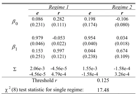
15 between the VARs governed by a function to be estimated. 11 _{Some switching models treat the} probabilities of regime changes as exogenous, some treat these probabilities as a function of exogenous variables, and some treat regime changes as triggered by the movement of an element of the VAR across a threshold.We opt for the latter type of model, known as a ―self-exciting threshold autoregression‖ (SETAR), because it allows the probability of a regime change to build when macro conditions are unsustainable, as for example, when exchange rate policy leads to an increasingly strong currency. Also, unlike the second type of switching mentioned above, the SETAR model allows the triggering variable itself to switch processes.

To implement the SETAR model, we assume the economy is in one of two macro regimes at any point in time. When regime m 

 

m t t m m t s s ₀ _{1 1} , where m m t m t E _    

_{ }  _{. Regime switches are triggered when one of}

the elements of the vector sthe interest rate, in our casecrosses an estimated threshold value. Estimates of this specification are reported in Table 2. They imply that the economy is regime 1 when the real interest rate is below 0.125 (12.5 percent), and in regime 2 otherwise. Also, the point estimates imply stable processes for in both regimes, but real interest rates are substantially higher in the second regime, and the peso tends to be weaker. 12 _{Finally, simulations of the} estimated SETAR show that the unconditional variance of the exchange rate process is higher in regime 1, while the unconditional variance of the interest rate process is roughly the same in both

11 _{Applications of regime-switching models to exchange rates include Engel and Hamilton (1990) and Bollen, et al}

(2000). Applications to interest rate processes include Gray (1996). We are unaware of papers that apply switching estimators to the joint evolution of exchange rates and interest rates, although Chen (2006) estimates an exchange rate switching model in which the interest rate affects the probability of a regime switch but does not enter the VAR directly. The methodology for estimating multivariate switching models is nonetheless well developed (e.g., Clarida et al, 2003).

12 _{We have not performed unit root tests. Caner and Hansen (2001) develop unit root tests for univariate threshold}

16 regimes. Thus, other things equal, risk aversion and reliance on business income will make households prefer regime 2, while indebtedness will make households prefer regime 1. We examine the question of which effect dominates for different types of households in section IV below.

It remains to estimate the spread between the lending rate and the deposit rate, . We identify this parameter as the mean difference between these two series over the sample period:  = 0.060. This figure is not unusual for Latin American economies, but it is several percentage points higher than the spreads typically found in high-income countries (Beck et al, 2000).

B. Estimating the profit function

To obtain estimates of the operating profits function, 





Given these assumptions, total revenue (G_it) and total variable cost (C_it) are:

13 _{This characterization of demand is consistent with CES preferences over product varieties, frictionless trade, and}

17              ( 1)/ 1/ exp ( 1)  ( 1)/ ( 1)/        _it it _{it it} it A u w k G , (9a)             / 1/ exp ( 1)  ( 1)/ ( 1)/        _it it _{it it} it A u w k C , (9b) where  (1) _and   

  ( 1). Conveniently, productivity shocks (u_it), the demand shifter (A_it), variable factor prices (w_it), and capital stocks (k_it) enter (9a) and (9b) in the same way, so cross-equation restrictions help to identify parameters, and the ratio of variable costs to revenues is simply  < 1.

Since the demand shifter, the productivity shock, and the factor price index are

unobservable at the firm level, we treat 1/ exp (_ 1) (1)/       it it it u w A as a Cobb-Douglas

function of the real exchange rate and serially correlated firm-specific shocks. Further, to allow for discrepancies between book values and true values, we assume that the log of observed variable production costs (lnCm) differs from the log of ―true‖ costs (ln C) by the measurement errorc.14 Then, defining (s_t,a_it) to be the minimum profit shock at which a firm continues operating (as implied by the dynamic programming problem in section II above), the following system of equations provides a basis for identification of profit function parameters and the transition density f(_it1|_it): it it t it e k G   ln  ln  ln _{0 1 2} (10a)

14 _{Among other things, this discrepancy reflects the fact that some wages are overhead expenses rather than variable}

production costs, inventory accounting does not accurately reflect the opportunity cost of inputs, and some costs that are recorded as overhead may vary with production levels. Since sales revenue (G) is straightforward to record and much less subject to measurement error we do not allow for errors in the values of this variable.

18 c it it it t m it e k C  ln  ln  ln   ln _{0 1 2} (10b) it it it     _1 (10c) )] , ( [ 1 _{it t it} it   s a    (10d)

Hereit ~ N(0,2), and itc ~ N(0,_2C ) are assumed to be independent, serially uncorrelated

shocks. Note that by equations (10a) and (10b), true operating profits before interest payments may be written as:





 , , = _(1_)exp



  

1 ,

whereδ is the rate of depreciation.

Selection bias and simultaneity bias complicate estimation of the parameters in (10a)-(10d). The former problem arises because firms that draw very low productivity shocks shut down (by 10d), and the shutdown point is different for entrepreneurs with different asset stocks.15 The latter problem arises because current period capital stocks are chosen after the current period productivity shock is observed.16 _{We develop a moments-based estimator related} to Olley and Pakes (1996) that deals with both problems. Details are provided in appendix 1.

Table 1 reports estimates of the profit function, the transition density f(_it1|_it), and the rate of depreciation, δ. The profit function and transition estimates are obtained by fitting the system (10a-d) to data on the population of apparel producers appearing in the annual manufacturing survey for a least two consecutive years between 1981 and 1991. The

15 _{Big firms continue operating at relatively low}

it

 values because the difference between firms’ continuation values and their scrap values is increasing in _it and k_it (Olley and Pakes, 1996).

16 _{This is true in Olley and Pakes (1996) as well, but they assume that output is a function of previous period capital}

19 depreciation rate is constructed as the simple average across all observations on active firms of current depreciation expenses to capital stocks.

The estimates are generally quite plausible. At 0.61, capital’s marginal revenue product is substantial, but it implies diminishing returns to capital investment—either because of finite demand elasticities in product markets or span of control problems.17 The exchange rate coefficient implies each percentage point of appreciation reduces earnings, costs and profits by about 0.37 percent points. Plant-specific profitability shocks exhibit strong serial correlationthe root of this process is around 0.90, and is highly significant. Finally, the difference between the revenue function intercept and the cost function intercept implies that firms keep about 20 cents of each dollar of revenue as gross operating profit.

C. Estimating the remaining parameters

Estimation strategy

A number of parameters remain to be estimated. These include the sunk entry cost, F, the per-period fixed operating cost, f, the credit market imperfection index, , the probability that a former entrepreneur encounters a new business opportunity, p, the risk aversion parameter, σ, exogenous household income, y, the average log wealth among new entrepreneurial households,

0

a , the variance in wealth among new entrepreneurial households, 2 0 a

 _{, and the ratio of total}

productive assets to fixed capital, .18 _{These parameters, hereafter collectively referenced as  =}

17 _{Since Bloom (2009) assumes constant returns to scale and a mark-up of 0.33, the elasticity of revenue with respect}

to scale in his model is approximately 0.75. Calibrating to U.S. data spanning all forms of business, and assuming competitive product markets, Cagetti and Di Nardi (2006) estimate the elasticity of output or revenue with respect to scale at 0.88.

18 _{We express asset stocks in logs to better deal with skewness. The parameter  is included in  because our survey}

20 (F, f, , p, σ, y, a0, a20,), are estimated using the simulated method of moments.

19

The logic behind the estimator is as follows. Taking 





, | ,

(e_t₁ r_t₁ e_t r_t

 as given, one can numerically solve the optimization problem in section II at any feasible  value. Then, using the resulting policy functions, one can simulate the cross-firm distribution of capital, profits, productivity, and debt for the apparel sector as it evolves through time.Defining m() to be a vector of moments that summarizes these joint distributions and their evolution, the discrepancy between these simulated moments and their sample-based counterparts, m , can be can measured as ()



 













E is the efficient weighting matrix. Our estimator is = arg min )

(

 . Defining Ω as the variance-covariance matrix of the data moments, we construct the efficient weighting matrix as W=[(1+1/S)Ω]-1 _{where S denotes the number of simulations.}20

Several issues arise in simulating m(). First, we must discretize the state space involved in order to use standard solution techniques for solving firms’ dynamic optimization problems. For the macro variables and the profit shocks, which are jointly normally distributed, we apply Tauchen and Hussey’s (1991) quadrature rules to the estimated transition densities.21 _{For capital} stocks and asset values, we create a discrete grid based on observed distributions.22 Second, we

19 _{The discount factor  is fixed exogenouslyusing the average interest rate implied by the SETAR process: =}

1/(1+0.142)= 0.875.

20_{The first term in W represents the randomness in the actual data and the second term represents randomness}

coming from the simulated data. Ω is calculated by block bootstrapping the actual data with replacement. We use S=50 with each of these panels of firms having independent draw of macro shocks. Lee and Ingram (1991) show variance-covariance matrix of simulated moments is (1/S)* Ω under the estimating null hypothesis.

21_{In the case of macro variables, we also must convert quarterly transition probabilities to annual transition}

probabilities by compounding the former.

21 need an algorithm for finding argmin(). The function () is neither smooth nor concave, so gradient-based algorithms fail to identify global minima. We therefore use simulated annealing, repeated using different initial values to ensure robustness. Third, we must construct an initial cross-household distribution for the profitability shocks, _it. We base this distribution on the steady state distribution for the profitability shocks from our estimated of profit function. Fourth, since the data set does not report firms’ borrowing levels, we must impute total debt for each observation. We do so using total interest payments (which are reported) divided by the market lending rate. Finally, it is necessary to make some assumptions about the number of households that might potentially start new apparel firms in each period. We assume that in the initial period there are 300 owner-households and we assume that 250 new households appear in the population of potential entrepreneurs each period. These figures essentially serve to fix the number of active firms.23

We use 23 moments of general industry characteristics to estimate . These include moments of the distribution of capital among entrants, aiming to identify entry costs and entrants’ asset distribution parameters; moments that characterize cross-firm distribution of debts; inter-temporal and cross-firm covariances, aiming to identify utility (risk aversion) and

econometric estimation, we use 10 discrete points for exchange rate, 10 for interest rate and 6 for profit shocks. There is a little sensitivity in the solution to the capital and asset discretization, but qualitatively the solution does not change.

23_{Let I}

0 be the number of owner-households in period 0, and let N be the number of new households we add to the

population each period. Then if the fraction of new households that creates firms is e and the fraction of owner-households that shuts down its firms every period is x, the population of owner-households in period t is

        _{ }    x x eN x I

It 0(1 )t 1 (1 )t . Thus, with stable rates of entry and exit, the current population approaches eN/x

as , and the size of the initial population becomes irrelevant. Similarly, the asymptotic entry rate and exit rate depend only on e and x. Experiments show that, holding other parameters fixed, variations in the number of new potential entrants per period have very little effect on the simulated moments.

22 credit market imperfection parameters; entry and exit rate moments; and moments of the distribution of capital and operating profit, aiming to identify costs parameters.

Estimates

Table 3 reports  estimates in the upper panel; the simulated moments that they imply are juxtaposed with corresponding data-based moments in the lower panel. Overall, the model does a good job of replicating the main features of our panel of apparel firms, including their size distribution, profit distribution, entry and exit rates, and borrowing patterns. All of the 23 simulated moments except for two have the same sign as their sample counterparts, and most are close in magnitude.

Turning to the key parameters, sunk entry costs amount to 168,713 in 1977 Colombian pesos, or $10,243 in current US dollars. 24 This figure is equivalent to13 percent of the value of the fixed capital stock for a firm of average size. Entry costs reflect the bureaucratic costs associated with creating a new firm, capital installation and removal costs, and any customizing of equipment and facilities that does not add to their market value. Their magnitude seems plausible, given the finding that bureaucratic costs alone amounted to 19 percent of Colombian per capita income in 2007 (World Bank, 2008). 25 Fixed costs are estimated to be 26,279 1977 Colombian pesos, or $1,595 current U.S. dollars These expenditures are incurred every year, regardless of production levels; they include various overhead expenses like insurance and

24 _{In 1977, there were 46.11 pesos per dollar. Also the U.S. GDP deflator was about 36 percent of its value in 2007.}

We use these two statistics to translate 1977 Colombian pesos into current U.S. dollars.

25 _{By way of crude comparison, Hurst and Lusardi (2004) report that in 1984 the median start-up equity investment}

23 marketing.

We estimate non-asset household income (y) to be 4,058 in 1977 pesos, or $246 in current dollars, and we estimate the average initial wealth of a new entrepreneur (assuming a lognormal distribution) is estimated at a0 = 114,800 in 1977 pesos, or $6,970 in current dollars. The average initial wealth of new entrepreneurial households suggests that new entrepreneurs have to borrow in order to create a new business. However, since there is significant variation around this mean (a₀ = 43,158), our results do not imply that those who actually create

businesses must leverage themselves heavily. With regard to household preferences toward risk, our estimate of the utility function parameter, ˆ1.85, is within the ranges of values typically obtained from studies of the intertemporal elasticity of substitution and coefficient of relative risk aversion.26

The estimated credit market imperfection index (ˆ0.97) is close to unity, implying that creditors view themselves as unable to seize collateralized assets in the event of default. Put differently, creditors view households as capable of absconding with nearly the entire value of their firms’ productive assets if they choose to do so. One should bear in mind that, since θ is identified by the borrowing levels of firms at different (υ,k) combinations, it will tend toward unity whenever the data indicate that borrowing levels are low at small, highly profitable firms. Hence, although information asymmetries and costly state verification are not part of our model, they may well help explain the large θ value that we estimate. In any case, our finding is consistent with the World Bank’s (2008) assessment that there are severe enforcement problems in Colombian credit markets (refer to footnote 8). Further, as the simulated moments indicate,

26 _{Estimates of the intertemporal elasticity of substitution, which corresponds to 1/σ in our model, are typically}

found to be in the range of .5 to 1 when household data on consumption is used (e.g. Blundell, Browning and Meghir (1994), Attanaiso, Banks and Tanner (2002)).

24 the model does a reasonably good job of explaining the borrowing patterns observed in the data. It predicts equilibrium borrowing at  = 0.97 because, by not defaulting, borrowers keep open the option of operating a business in the future without incurring entry costs.

IV. Industry Structure, Wealth Distributions and Credit Market Imperfections

Given all of the parameter estimates discussed above, we can now use simulations to answer four basic questions. 27 First, how might industry and household characteristics change if loan contracts were perfectly enforceable? Second, how do credit market imperfections affect industry and household characteristics during regime 1 (strong but volatile exchange rate and low interest rates) versus regime 2 (weak, relative stable exchange rate and high interest rates)? Third, how do the effects of credit market imperfections depend upon the overall volatility of the macro environment? And finally, how has the large spread between borrowing and lending rates affected industry and household characteristics?

A. Ability to Enforce Debt Contracts

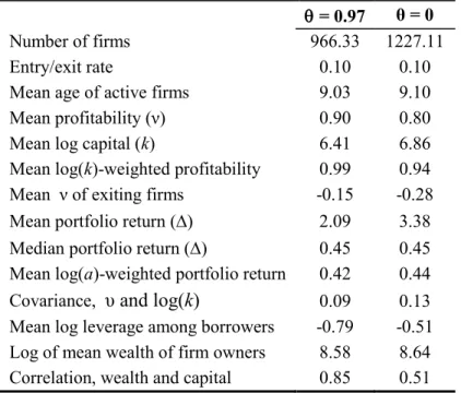
To summarize industry characteristics under different credit market conditions, we generate 50 simulations of the model under the ―base case‖ assumption that  = 0.97, and 50 simulations under the ―counterfactual‖ assumption that  = 0.28 The former implies that lenders are almost completely unable to recoup any collateral from a defaulting borrower, while the

27 _{To perform these simulations, it is necessary to assume an initial distribution of potential entrant firms over asset}

levels, hN(a_it), and an initial distribution of incumbent owner-households over asset levels and productivity levels, hI(a_it,_it). We let the former be lognormal with the estimated parameter values reported in table 3, and we let the initial distribution of incumbents’ wealth distributed lognormally with mean 6 and variance 2. Since we discard the first 30 years of simulated data, the results proved to be insensitive to the initial wealth distribution of incumbents.

28 _{The same sets of draws for profit shocks (ν’s) and macro shocks (υ’s) are used in both sets of simulations, so the}

25 latter implies they can seize a defaulting borrower’s collateral and sell it at its full market value. All simulations are for 130 periods. After discarding the first 30 periods of each (to eliminate atypical ―burn-in‖ years), we construct cross-simulation average moments under each scenario.

Table 4 summarizes the results. Note first that reducing  from 0.97 to 0.0 increases the average log debt-to-asset (leverage) ratio among borrowers from -0.79 to -0.51, or taking antilogs, from .45 to .60. This extra borrowing reflects the expansion of firms owned by low-a, high-ν households toward the size at which the marginal return on business capital (k) matches the lending rate.

As households leverage their businesses they increase the rate of return on their asset portfolio:





The wealth-weighted average of this statistic,





i it i it it

a

a / , rises from 0.42 to 0.44 when 

drops from 0.97 to zero, indicating a 2 percentage point improvement in the return on the pooled wealth portfolios of entrepreneurial households (Table 4). 29 _{These gains are concentrated among} the low-a households, as evidenced by the dramatic increase in the unweighted average  value. In fact, since the median  value is unresponsive to improvements in contract enforceability, it appears that the return on wealth for the majority of entrepreneurs is unaffected.

In addition to increasing income among low-a owner-households, perfect contract enforceability affects the aggregate economy in several respects. First, it induces higher savings rates among the affected owner-households, causing the average log wealth level to rise from

29 _{The typical  value is above the interest rate, even when  =0, since operating profits must be large enough in}

expectation to finance entry costs. Further, since entry costs are the same for all households,  is typically larger among low-a entrepreneurial households, for whom the denominator of (11) is relatively small.

26 8.58 to 8.64 and the average log capital stock to rise from 6.41 to 6.86. Second, by moving financial resources toward relatively high-return firms, it improves allocative efficiency. This is apparent in the increased covariance between size and profit shocks and in the diminished correlation between wealth and firm size.

Finally, as θ drops from 0.97 to 0.0, more low-a potential owner households find it worthwhile to open businesses, and more low-a owner-entrepreneurs find it worthwhile to stay in business. These adjustments are reflected in the number of active firms, which increases from 966 to 1227, in the average life span of firms, which rises from 9.03 years to 9.10 years, in the average ν among owner-entrepreneurs, which falls from 0.90 to 0.80, and in the average profit shock among exiting firms, which falls from -0.16 to -0.21.

B. Loan enforcement effects under alternative Colombian macro regimes

Next we investigate whether the effects of credit market imperfections are similar during the different macro regimes identified by our switching VAR. We do this by generating 50 simulations of our model, each for 130 periods, discarding the initial 30 periods as a burn-in. Then we average values of the various statistics for all periods during which regime 1 prevailed, and for all periods when regime 2 prevailed. Households are presumed to correctly perceive that switching patterns are governed by the estimated switching threshold of r = 0.125.

The first two columns of table 5 summarize the regime 1 and regime 2 results for the base case of θ = 0.97 and the last two columns do the same for the counterfactual case of θ = 0. Note that the average log exchange rate and interest rate are 4.70 and 0.09, respectively, in regime 1, while they are 4.59 and 0.16, respectively, in regime 2. Thus interest rates and exchange rates move in opposite directions when regimes change, and their effects on businesses’ net earnings after interest work in opposite directions. Nonetheless, on average entrepreneurs earn higher

27 returns on their wealth under the strong exchange rates and low interest rates of regime 1. Further, since the payoff to low interest rates depends upon firms’ ability to borrow, the effects of regime switches are highly dependent upon contract enforceability. The difference between weighted average earnings rates on portfolios under the two regimes is only 3 percentage points when credit markets function poorly (=0.97), but when contracts are perfectly enforceable (=0) it is 17 percentage points.

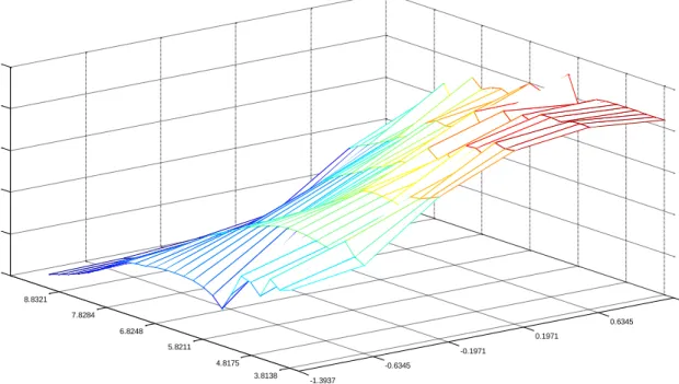
Figure 3a depicts the percentage changes in welfare for different types of incumbent owner-households as the economy moves from regime 2 to regime 1, presuming that θ = 0.97. Clearly the net gains from switching to regime 2 tend to fall with productivity and rise with household wealth. This pattern reflects the fact that regime 1’s high interest rates help households that are net depositors, while regime 2’s favorable exchange rates increase the operating profits of business owners. Since low- households don’t hold much of their wealth in businesses and are relatively likely to trade their businesses for bank deposits in the future, their primary concern is with deposit rates. High wealth households likewise hold relatively large fractions of their wealth in banks and do well when deposit rates are high.

Among incumbents who are more dependent upon business income—that is, low-a, high- entrepreneurs—several more effects come into in play. First, these entrepreneurs dislike the extra exchange-rate-induced volatility in operating profits that comes with regime 1. This is particularly true for incumbents with low wealth, who are relatively risk-averse. Second, at any given wealth level, high-ν incumbents are less bothered by low interest rates because they hold a relatively large share of their assets in the form of business investments. In fact, low-a, high-ν households tend to be debtors, so they welcome the lower lending rates that regime 1 brings. The

28 interaction of these effects makes the welfare effects of regime switches non-monotonic in ν at low a values.

Figure 3b shows how the surface in figure 3a would shift if contract enforceability were perfect (θ=0). High-a, low- households are not affected by θ because these households self-finance their capital investments and are not credit constrained when contract enforcement is weak. However, improvements in enforcement do help low-a, high-ν households in periods when they would like to be borrowing more, i.e., when regime 1 prevails.30 _This enforcement-induced shift in the value of low-a, high-ν households is associated with more regime-1 business investment by households with modest wealth, and it is the reason that cov(a,k) is higher under regime 2 than under regime 1 when θ = 0 (Table 5).

C. Contract Enforcement and the Macro Environment: Argentina versus Colombia Results in the previous section suggest that the effects of improved contract enforceability depend partly upon the degree of macro volatility. To further explore this relationship, we now ask how changes in θ would have affected Colombian households if they had been somehow transplanted to the relatively volatile Argentine macro environment.

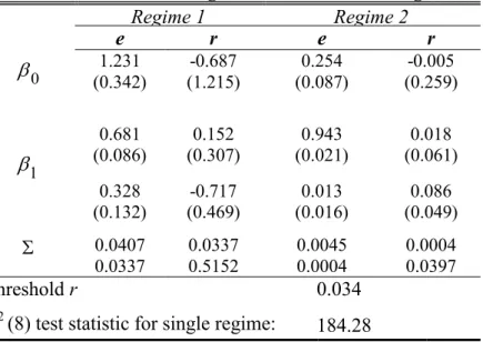
Figure 4 shows the evolution of Argentine real exchange rates and real interest rates over the past 30 years. Juxtaposed with figure 1, it demonstrates that this country’s recent macro history has been much more turbulent than Colombia’s. This impression is confirmed by estimates of our SETAR switching model based on Argentine time series (Table 7). We decisively reject a single regime, and we estimate a covariance matrix for the innovations in the process that is roughly 10 larger than Colombia’s (compare Table 7 to Table 1).

30 _{This finding is similar to Gine and Townsend’s (2004), whose simulations imply that the primary beneficiaries of}

improvements in the Thai financial sector are ―talented would-be entrepreneurs who lack credit and cannot otherwise go into business (or invest little capital).‖ (p. 269)

29 Table 7 repeats the counterfactual experiment that generated Table 4, replacing the Colombian transition density for st from Table 1with the Argentine transition density from Table 6. All other parameters are left unchanged. In a number of respects, we find that well-functioning credit markets are more important when interest rates and exchange rates are volatile. Compared to the findings for the Colombian macro environment, Argentine macro conditions induce larger responses to perfect enforcement in terms of leverage rates, average firm life spans, average portfolio returns, average log firm sizes, and average log wealth levels. The reason is that with relatively dramatic macro shocks, households have stronger incentives to create or expand firms during good times and to contract or shut them down during bad times. Well-functioning credit markets allow them to do this.

Surprisingly, while the weighted average return on portfolios rises in response to improved contract enforcement in the Colombian macro environment (Table 4), it drops when Argentine macro conditions are assumed (Table 7). What might explain this contrast? When improvements in contract enforceability make it easier to finance entry and expansion, more firms avail themselves of the temporary profit opportunities created by the volatile Argentine macro environment. Accordingly, marginally profitable firms are more numerous when θ = 0 than when θ = 0.97, and the weighted-average return on portfolios falls. This interpretation is supported by the large drop in average profit shocks and average life expectancy of firms.

D. The Effects of the Borrowing/Lending Spread

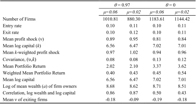
As a final exercise, we explore the effects of more efficient financial intermediation in a different sense: lower spreads between borrowing and lending rates, μ. For non-entrepreneurial households, it can be seen from (1) that the first order effect of a small reduction in μ is to raise

30 the value of current income by an amount proportional to the household’s asset holdings, a. For owner-households with bank deposits, (4) show that a reduction in μ has the first order effect of reducing consumption by an amount that is proportional to . For owner-households with debt, (4) shows that the reduction in the spread has no effect on income—all of the household’s assets are invested in the firm and receiving a return of r. Thus, one of the effects of reducing the spread should be to make exit more attractive for incumbent firms by raising the return on assets held by non-entrepreneurial households. This should raise the threshold value of ν required for a firm to remain in the industry, with this effect more pronounced for wealthy households.

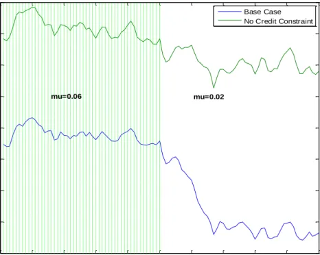
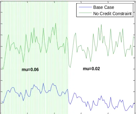
To examine the impact of a reduction in μ on the Colombian apparel industry, we simulate our model forward under a base case scenario (μ=0.06) and a counterfactual scenario (μ=0.02). The reduction in spreads induces different savings patterns, and the associated changes in wealth trajectories generate a gradual change in industry structure, so for this exercise we go beyond before/after comparisons to explore transition dynamics. More precisely, we simulate the first 50 periods with μ=0.06 and an additional 50 periods with μ=0.02, discarding an initial burn-in period of 30 years. We assume that the reduction burn-in spread is unanticipated, but once it has occurred, households correctly understand that the reduction is permanent.

Figure 5a shows the adjustment in the number of firms that takes place after the spread reduction in period 50. The higher deposit rate attracts wealth out of proprietorships and into bank accounts, but the adjustment is gradual because it is accomplished mainly through reduced entry rates during a transition period. This asymmetry in adjustment margins reflects the presence of sunk entry costs, which induce some entrepreneurs to continuing operating firms after the jump in deposit rates, even though they would not have created their firms if they had

31