Banco Central de Chile
Documentos de Trabajo
Central Bank of Chile
Working Papers
N° 606
Enero 2011
COLLEGE RISK AND RETURN
Gonzalo Castex
La serie de Documentos de Trabajo en versión PDF puede obtenerse gratis en la dirección electrónica:
http://www.bcentral.cl/esp/estpub/estudios/dtbc. Existe la posibilidad de solicitar una copia impresa con un costo de $500 si es dentro de Chile y US$12 si es para fuera de Chile. Las solicitudes se pueden hacer
por fax: (56-2) 6702231 o a través de correo electrónico: [email protected].
Working Papers in PDF format can be downloaded free of charge from:
http://www.bcentral.cl/eng/stdpub/studies/workingpaper. Printed versions can be ordered individually for US$12 per copy (for orders inside Chile the charge is Ch$500.) Orders can be placed by fax:
BANCO CENTRAL DE CHILE
CENTRAL BANK OF CHILE
La serie Documentos de Trabajo es una publicación del Banco Central de Chile que divulga
los trabajos de investigación económica realizados por profesionales de esta institución o
encargados por ella a terceros. El objetivo de la serie es aportar al debate temas relevantes y
presentar nuevos enfoques en el análisis de los mismos. La difusión de los Documentos de
Trabajo sólo intenta facilitar el intercambio de ideas y dar a conocer investigaciones, con
carácter preliminar, para su discusión y comentarios.
La publicación de los Documentos de Trabajo no está sujeta a la aprobación previa de los
miembros del Consejo del Banco Central de Chile. Tanto el contenido de los Documentos
de Trabajo como también los análisis y conclusiones que de ellos se deriven, son de
exclusiva responsabilidad de su o sus autores y no reflejan necesariamente la opinión del
Banco Central de Chile o de sus Consejeros.
The Working Papers series of the Central Bank of Chile disseminates economic research
conducted by Central Bank staff or third parties under the sponsorship of the Bank. The
purpose of the series is to contribute to the discussion of relevant issues and develop new
analytical or empirical approaches in their analyses. The only aim of the Working Papers is
to disseminate preliminary research for its discussion and comments.
Publication of Working Papers is not subject to previous approval by the members of the
Board of the Central Bank. The views and conclusions presented in the papers are
exclusively those of the author(s) and do not necessarily reflect the position of the Central
Bank of Chile or of the Board members.
Documento de Trabajo
Working Paper
N° 605
N° 605
COLLEGE RISK AND RETURN
‡
Gonzalo Castex
Gerencia de Investigación Económica Banco Central de Chile
Abstract
Attending college is thought of as a very profitable investment decision, as its estimated
annualized return ranges from 8% to 13%. However, a large fraction of high school
graduates do not enroll in college. I reconcile the observed high average returns to
schooling with relatively low attendance rates when considering college as a risky
investment decision.
A high dropout risk has two important effects on the estimated average returns to college:
selection bias and risk premium. In order to explicitly consider the selection bias, I explore
the dropout risk in a life-cycle model with heterogeneous ability. The risk-premium of
college participation accounts for 21% of the excess returns to college education for
high-ability students and 19% of the excess return for low-high-ability students. Risk averse agents
are willing to reduce their return to college in order to avoid the dropout risk. The effect is
not uniform across ability levels.
Resumen
Los estudios universitarios son considerados una inversión rentable, con retornos estimados
que varían entre 8% y 13% anual para el caso de Estados Unidos. Sin embargo, una gran
fracción de los estudiantes que terminan la educación secundaria no continúa a la educación
universitaria. Al considerar el riesgo involucrado en la decisión de continuar con educación
universitaria, se hacen compatibles los hechos mencionados.
Una alta tasa de deserción universitaria tiene dos importantes efectos sobre los retornos
promedio estimados: sesgo de selección y premio por riesgo. Con el objeto de considerar
explícitamente el sesgo de selección, se analiza el riesgo de deserción en un modelo de
ciclo de vida con agentes que difieren en su nivel de habilidad. El premio por riesgo de
proseguir la educación universitaria explica el 21% del exceso de retorno a la educación
para estudiantes de alto nivel de habilidad y 19% para los estudiantes de bajo nivel de
habilidad. Agentes adversos al riesgo están dispuestos a reducir el retorno a la educación
universitaria con el fin de mitigar el riesgo. El efecto no es uniforme para todos los niveles
de habilidad.
Special thanks are due to Yongsung Chang for his advice, encouragement and support in this and other projects. I also thank Geni Dechter and Andrew Davis for useful comments and participants at EALE and SOLE Conference in 2010 and Bank of Israel Seminar. All errors are my own. Correspondence: [email protected]
1
Introduction
Attending college is considered a very profitable investment, as its estimated annualized return ranges from 8% to 13% (see for example Card, 1999). However, a large fraction of high school graduates do not enroll in college. According to the National Longitudinal Sample of Youth 1979 (hereafter NLSY79), 59% of high school graduates do not continue formal education. Moreover, around 30% of high school graduates from the highest quartile of the cognitive ability distribution, measured by AFQT scores, do not enroll in college. This occurs despite the availability of student loan funds for financing college and the fact college returns highly compensate the earnings forgone while in college (Ionescu 2009).
Selection bias is a common explanation used by the existing literature to explain the high return to college. Different schooling levels may be attributed to differences in individual aptitudes and tastes for schooling relative to work (Card 2001). An environment in which college education is risky can reconcile low attendance rates with a high return to college education.
Previous literature often omits an important factor about the college investment decision: the risk. According to Restuccia and Urrutia (2004) and Mayer (2008), the average college dropout rate is around 45%-55%.1 This high dropout risk affects the estimated average returns to college in two important ways: selection bias (as in the traditional literature by Willis and Rosen (1979), and Card (2001)) and risk premium.
According to the NLSY79, the college dropout rate is about 55%. The average tuition paid per year by students who dropped out was, at the beginning of the 1980s, $3,300. 5% of this group paid more than $10,000.2 In average, students who drop out owe $9,350 to financial and educational institutions; 15% of
this group owes more than $24,000. The college participation decision seems not always to be optimal, in particular for students who dropout and have large accumulated debts from financing college.
Taking into account dropout risk allows me to explicitly consider the selection bias and the individual-ability effect on the risk premium.3 I explore the dropout risk in a life-cycle model with heterogeneous ability.
The model is calibrated to match college participation rates and dropout rates observed in NLSY79. Under this model specification, I evaluate the role played by dropout risk for each level of ability and quantify how much of the return to college education, measured as college premium, is explained by its risk. The risk
lowest quartile of the ability distribution, and about 21% of the return to college education for students from the highest quartile of the ability distribution
The rest of the paper is organized as follows: Section 2 describes the model. The data and my calibration strategy are described in section 3. Section 4 presents results. Section 5 concludes the paper.
2
A life-cycle model with heterogeneous ability
In this section I analyze the role played by heterogeneity in ability level and its interaction with risky college investment. The model is built and calibrated considering college dropout as a source of uninsurable risk after college enrollment. The model reproduces wage distributions by educational and ability levels, college participation and dropout rates by ability levels as observed in the data.4 A second simulation of the model is performed without considering the dropout risk, students who enroll successfully graduate from college. The non-risky college environment generates larger enrollment rates across all ability levels, since life time utility is higher for students from all ability levels. Then, I adjust the college premium to match the participation rates observed in the data for each ability level, obtaining a measure of return to college in environments with and without dropout risk, these returns reproduce the same attendance rates across the ability distribution. I interpret the differential return between these two environments as an estimate of risk premium.
2.1
The model
In this section I describe the model used to explain to what extent the return to college is explained by its risk and evaluate the role played by heterogeneous ability. I develop a three stage life-cycle model with a discrete choice of college enrollment and exogenous college dropout. I assume that the economy is populated by a unitary mass of heterogeneous agents that derive instantaneous utility solely from consumption. Schooling decisions are made in the first stage and are based on the lifetime utility maximization problem that each agent faces. Individuals may obtain three levels of education: no college, some college and college education. Education and employment are mutually exclusive in each period.
The life-cycle of an agent has three different phases. In the first phase, agents draw their type, a pair 4The model is also calibrated to match moments with respect to family income, but integrated out over this variable.
{x, y} ≡Ω, that corresponds to ability and family income levels from the joint distributionH(x, y), x∈[x,
x]≡ Φ, y ∈[y, y] ≡ Γ and H: Φ×Γ →[0,1]2. The second dimension in individual heterogeneity, family
income, is included primarily for calibration purposes. Results are integrated out over this variable. In this stage agents decide whether to enroll in college or join the labor force. This decision is a function of their type and current wage offer. Agents receive this wage offer from the non-college wage distribution,
wN ∼FN(w). They simultaneously observe the probability of dropping out and the wage distributions of
college graduates and college dropouts. The dropout probability is a function of individual types,ψ=ψ(Ω). I assume that individuals have perfect foresight about the skill price distributions and that wages depend on ability and are constant over the life-cycle. With the high-school wage offer in hand and observable college-success probability, college-graduate and college-dropout wage distributions, agents make their decisions about college attendance and labor market participation.
The decision for agenti about whether or not to participate in college at the first stage is based on the following optimization problem: V(Ωi;wNi ) = max{VC(Ωi), VN(Ωi;wiN)}, where VC(Ωi) is the life-time
utility of attending college andVN(Ω
i;wNi ) is the life-time utility of not attending college.5
Agents who attend college during the first stage consume c and are allowed to borrow at a subsidized interest rate,ρ; they also have to pay a college tuition cost, which equalsτ. In order to finance their education, students receive grants and scholarships which are a function of ability and family income, represented by
g(Ω). These agents also receive instant utility from college attendance, φ(Ωj). This utility is treated as a
residual in the model since it is not measured in the data and is a function of an effort cost of college and the consumption value of schooling in utils. φ(.) has an important interpretation as the consumption value of schooling, summarizing non-pecuniary benefits of acquiring college education. The natural borrowing limit is also imposed to rule out Ponzi schemes.
The discounted life-time utility of college attendees of type Ωj is given by the following expression:
VC(Ωj) = max c,a0 u(c) +φ(Ωj) +β Z w {ψ(Ωj)VCS(Ωj, a0) + (1−ψ(Ωj))VCD(Ωj, a0;w)}dFCD(w) (1) s.t. c+ρa0I(a0<0)+a0I(a0>0)+τ(Ωj) =g(Ωj) a0 >−a
College attendees derive utility from consumption and discount future utility at rateβ. They maximize life-time utility subject to budget and borrowing constraints. Agents successfully graduate or dropout from college in the second stage of their life-cycle, with probabilitiesψ(Ωj) and 1−ψ(Ωj), in which case their
discounted life-time utilities are given byVCS(Ω
j, a0) andVCD(Ωj, a0;w), respectively.
Equation (1) also describes the trade off faced by high school graduates when making the college enroll-ment decision. Graduating from college is associated with a higher expected wage, but the cost of financing education may lead to negative asset holdings. The additional potential for dropout, makes college enroll-ment a risky investenroll-ment decision. Individuals who attend college in the first period but drop out in the second period are likely to receive a lower wage offer and may have accumulated debt when they join the labor force.
Agents who choose not to enroll in college in the first stage of their life-cycle and join the labor force after high school graduation face a consumption-saving decision problem described by:
VN(Ωj;wjN) = max c,a0 u(c) +βW a0;wNj (2) s.t. c+a0=wNj a0 >−a
Agents who decide to join the labor force consume c, borrow or save a0 and receive ability-dependent wage compensation. They face the natural borrowing limit and discount future utility at rate β. W(a;w) corresponds to a life-time utility of agents at the working stage. The value of W(a;w) is obtained through
a standard consumption-saving utility maximization problem with no uncertainty, where the state variables are the asset/debt level and wage. A complete description ofW(a;w) is provided in equation (5).
The life-time utility of individuals without college education increases with wage. On the other hand, receiving a higher wage offer in the first stage of the life-cycle reduces the probability of college enrollment.
In the second phase of their life-cycle, agents who are enrolled in college face the dropout risk, with probability ψ(Ωj) agents successfully graduate college and obtain utility defined by VCS(Ωj, a0). With
probability 1−ψ(Ωj) agents dropout, in which case agents draw a wage from the college-dropout wage
distribution and obtain a life-time utility described byVCD(Ωj, a0;w).
If agents continue college, they will continue paying tuition, will receive grants and will be allowed borrow at the subsidized interest rate in the second stage of their life-cycle. Agents continue deriving utility from college as in the previous stage. The maximization problem of a college student in the second stage of the life-cycle takes the following form:
VCS(Ωj, a) = max c,a0 u(c) +φ2(Ωj) +β Z w W(A;w)dFC(w) (3) s.t. c+ρa0I(a0<0)+a0I(a0>0)+τ(Ωj) =g(Ωj) +a(1 +r)I(a>0) a0>−a aI(a<0)+a0=A A>−a
Note that in the maximization problem, the borrowing constraint faced by the agent considers the total accumulated debt,A.
Agents who drop out after spending the first stage of their life-cycle in college have to pay their accu-mulated debt. In each remaining period of their life-cycle they maximize a consumption-saving problem,
VCD(Ωj, a;w) = max c,a0 {u(c) +βW(a 0;w)} (4) s.t. c+a0 =a(1 +r) +w a0>−a
The third stage of the life-cycle is the working stage for those who graduate from college; the working stage arrives earlier for those who decided not to enroll or for those who receive the dropout shock. For simplicity it is assumed that the dropout shock arrives in the middle of the college education process.
Agents who graduate from college draw a wage from the college wage distribution,wC ∼FC(w). In the
following periods they face a consumption-saving problem, given by W(a, w). The life time utility at the third stage of the life-cycle is a function of acquired education in the earlier periods. It is specified as follows:
W(a, w) = max c,a0 {u(c) +γβW(a 0, w)} (5) st. c+a0=a(1 +r) +w a0 >−a
Equation (5) describes the consumption-saving problem agents face when they join the labor force. I include the survival probability γ to match the expected duration of labor force participation (and the retirement age). The maximization problem is solved given the budget constraint and natural borrowing limit. Utility in the working stage is increasing in assets and wages. Since wages are ability dependent, the life-time utility is also increasing in ability level.
3
Data and Calibration
3.1
Data
The analysis uses data from the National Longitudinal Survey of Youth 1979 cohort. It provides a nationally representative sample of young men and women aged 14-22 at the beginning of 1979. For the individuals in the sample, college attendance decisions took place in the early 1980s. excluding youths who are part of the minority and poor white oversamples (I use only the full random samples in the analysis). The data contains detailed information on individuals, including their ability level, family income and other family and personal characteristics.6
The data source contains a measure of ability, Armed Forces Qualification Test - AFQT scores, widely used in the literature as a measure of cognitive achievement, aptitude and intelligence. I use the AFQT89 variable as a proxi for cognitive ability.7
Another key variable in this analysis is family income. NLSY79 reports family income measured in early survey years. I use average family income when respondents are ages 16-17.8 I denominate the family income
measure in 2007 dollars using the consumer price index for all urban consumers.
Within the sample, college attendance and dropout decisions took place in the early 1980s. Following Belley and Lochner (2007), an individual is considered to have attended college if their highest grade attended is equal or greater than 13. Similarly, it is considered a college dropout if the agent attends college but does not graduate.
The raw NLSY79 contains information on 6,111 individuals.9 Individuals with no information about
AFQT scores, family income or schooling were dropped from the sample. The final sample contains 2,477 individuals. Descriptive statistics for the variables used in the analysis are provided in Appendix B.
6See Appendix B for summary statistics.
7AFQT89 is not adjusted by age. I thank Lance Lochner for pointing this out. I follow the age-correction procedure
suggested by Carneiro et al. (2005).
8When income is available only for age 16 or age 17 and not both, I use the available measure. 9Considered only the cross-sectional representative sample.
3.2
Calibration
The proposed model is calibrated to match college participation, college dropout and wage distributions observed in the data.
This section discusses the choice of parameters used in the model. The model has a set of 18 parameters. I divide the parameter space into three subsets. The first corresponds to parameters that I impose in the model from pre-existing estimates in previous literature. The second set corresponds to parameters estimated directly from the data. I calibrate the remaining parameters to match certain moments in the sample.
External parameters: The first subset of parameters and their values are reported in table 1.
I use a CRRA utility function with coefficient of risk aversion σ. Agents enter the first stage as an 18-year-old high school graduate. The duration of the first and second stages of the life-cycle is two years each; during the first period agents make their college enrollment decision. The third stage has an infinite horizon; I add a survival probability to the specification to match the retirement age.
Parameter Value Target/Source Coeff. of risk aversion σ 2 standard Discount factor β 0.96 standard Prob. to survive γ 0.957 to match 65 yrs. Interest rate r 4% standard Subsidized int. rate ρ 0.9246 to setrt=1= 0
Table 1: Imposed parameters in the model
The coefficient of risk aversion, the discount factor and the interest rate are chosen following standard practice in the literature. I use a survival probability in the third stage (working stage) maximization problem to match a retirement age of 65 years. Finally, the subsidized interest rate was chosen to create a zero cost for those agents who borrow to finance their education.
Estimated parameters: The second subset of parameters are estimated from the data set. They
include the tuition cost, grants awarded and the ability/family income distribution.
I follow the previous literature and estimate an average tuition (Akyol and Athreya 2005, Caucutt and Kumar 1999, Gallipoli et al. 2007, Garriga and Keightley 2007). Tuition is reported only in 1979. The annual average tuition cost is estimated to be $4,350 (2007 dollars).
suggest a linear specification in ability and family income. Using data from NLSY79 I estimate the following equation for log-grants:
g(Ωi) =α0+α1xi+α2yi+θXi+αλλbi+εi, (6)
whereXi is a set of controls for individual and family characteristics.
To estimate the above equation requires correction for selection bias: grants are not observed for those high school graduates who do not enroll in college. To correct for this selection, I implement the conventional two-step selectivity adjustment procedure suggested by Heckman (1979). In the first stage I formulate an econometric model to estimate the probability of attending college, which is used to predict the probability of college enrollment for each individual, λbi.10 In the second stage, I correct for the selection problem by
including the predicted individual probability as an additional explanatory variable in the grants specification. See Appendix C for details, parameter values and estimated effects of individual and family characteristics on college attendance. The parameters of interest are reported in the following table and estimation results show that grants increase in ability and decrease in family income.
Grants constant ability f amily income
NLSY79 11.40 0.23 -0.35 (1.99) (0.11) (0.18) Table 2: Parameters estimated for grant equation
To solve the model I impose the joint probability distribution of ability and family income observed in NLSY79. Ability is normalized to have zero mean and standard deviation equal to one. Family income is expressed in natural logs. Figure 1 shows the marginal densities:
Calibrated parameters: The third subset of parameters is calibrated using simulated method of
moments. I calibrate parameters of the wage distributions, probability of college success and the college utility function to match key moments observed in the data.
Wage distributions are calibrated to match means and standard deviations of life-cycle wages for each ability and educational level. Probability of college success is calibrated to match average dropout rates by ability and family income levels. College utility, which I assume to have a linear specification in ability and
0 .1 .2 .3 .4 De ns it y -2 -1 0 1 2 AFQT 0 .2 .4 .6 .8 De n s it y 8 9 10 11 12 FI
Figure 1: Marginal densities NLSY79: (a)Ability, (b)Family Income distributions
I use the NLSY79 data to obtain wage distributions for high school graduates, college graduates and college dropouts. The annual mean wage is $22,549 for high school graduates, $25,399 for those who drop out from college and $29,158 for college graduates.11 The underlying college premium is consistent with the
one reported by Goldin and Katz (2007) who use the 1980 Current Population Survey (CPS).
To generate the model wage profile, I estimate the return to ability and experience for different educational levels.12 These estimates are used to project wage profiles along the life-cycle for different ability and
education groups. I use the estimated wage paths to calculate a mean wage and its standard deviation for each ability and education level. Parameter estimates are reported in Appendix C.
At each educational level agents receive ability dependent wage offers. I define the wage offer function as follows: weduc=$
0+$1xi+εw. I assume that these wage offers are constant throughout each agent’s life
and are generated such that the accepted wages for each ability and educational level match the mean and standard deviation of the life-cycle wages estimated in the data.
Probability of college success is a function of the agent’s type. The probability parameter was calibrated to match dropout rates observed in the data per each ability and family income group. The college utility parameters are not measured in the data and are considered as a residual in the model. These parameters are calibrated such that the model reproduces some relevant features observed in the data, particularly the college attendance rates for each ability level. Appendix C summarizes the parameters estimated from the model.
Calibration results: Here I document how the model performs by comparing model generated statistics
with those observed in the data.
11See Appendix C for details. Wages are nominated in 2007 dollars. 12I use the standard Mincer approach.
Grants and scholarships from the model and data are reported in the following table.13
Grants Data Model NLSY79 2,128 2,394 (556) (819) Table 3: Annual grants: Model vs. Data
As can be seen from Table 3, the model slightly overestimates average and standard deviations for annual grants and scholarships observed in the data (values are nominated in 2007 dollars).
The following tables show mean log wages by ability quartile and educational levels. 1980
Ability quartile Model Data lowest - Q1 10.030 10.049 (0.62) (0.63) Q2 10.164 10.196 (0.62) (0.63) Q3 10.324 10.360 (0.62) (0.63) highest - Q4 10.513 10.517 (0.62) (0.63)
Table 4: Average log-wage for college graduate
Note: Average wage over the life-cycle for different ability levels, measured as AFQT score. Standard
deviation in parentheses. Source is NLSY79.
Table 4 shows that the model performs well in replicating the wage premium for each ability level. High-ability college graduates (Q4) from the model get a 48% higher wage relative to those of low-High-ability level (Q1). The wage structure for high school graduates is reported in the following table:
As can be seen in table 5, in the high school wage distribution the ability premium is lower compared to the one for college graduates, and it is approximately 36%.
4
Results
1980 Ability quartile Model Data
lowest - Q1 9.855 9.828 (0.64) (0.68) Q2 9.964 9.952 (0.69) (0.68) Q3 10.090 10.091 (0.68) (0.68) highest - Q4 10.237 10.224 (0.70) (0.68)
Table 5: Average log-wage for high school graduates
Note: Average wage over the life-cycle for different ability levels, measured as AFQT score. Standard deviation in parentheses. Source is NLSY79.
participation and dropout rates outcome’s from the model and comparison with the data is shown in figure 2.
College Participation Rates
0% 10% 20% 30% 40% 50% 60% 70% 80%
AFQT Q1 AFQT Q2 AFQT Q3 AFQT Q4
Model Data
College Dropout Rates
0% 10% 20% 30% 40% 50% 60% 70% 80% 90%
AFQT Q1 AFQT Q2 AFQT Q3 AFQT Q4
Model Data
Figure 2: College Participation and College Dropouts rates
The outcome of a model with no college utility parameter (φ(Ωj)) is of practical interest and is presented in
Appendix D. The results show that this simpler model reproduces 45% of the overall college participation rate observed in NLSY79. Figure 4 in Appendix D demonstrates that college participation rates are overestimated for low-ability students and underestimated for high-ability students. These results suggest that low ability individuals have some disutility from attending college, while high-ability students gain utility from college participation. Alternatively, it is possible that students who attend college must exert some effort which is decreasing with ability level.
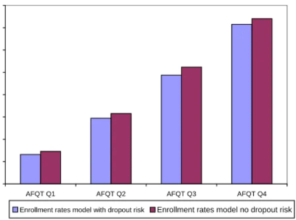
The matched participation rates for 1980 are shown in Figure 2, termed here as the risky allocation, which serve as a starting point for the risk premium measurement. To quantify to what extent the dropout risk can explain the return to college observed in the data, I update the simulation of the model without considering the dropout risk: if a high school graduate decides to attend college, he/she will successfully graduate. In this environment,ψ(Ωj) = 1∀Ωj. This alternative specification increases the life-time utility of
college participation since all agents receive the college premium with certainty. This implies that enrollment rates increase for the entire ability profile. I name this college participation profile the non-risky allocation. College participation rates in an environment with and without dropout risk are presented in figure 3.
Uncertainty Effect on Enrollment Rates
0% 10% 20% 30% 40% 50% 60% 70% 80%
AFQT Q1 AFQT Q2 AFQT Q3 AFQT Q4 Enrollment rates model with dropout risk Enrollment rates model no dropout risk
Figure 3: Dropout Risk Effect on College Enrollment Rates
To measure how much of the return to college observed in the data is due to risk premium, I adjust the college premium downwards in the model specification with no dropout risk, as depicted in Figure 3, such that college participation decreases from the non-risky allocation to the risky allocation profile. The amount of adjustment in the college wage premium corresponds to a quantification of the risk premium. The following table shows the college premium of the model with risk and without risk required to generate the participation rates from the risky allocation. The college premium is measured as the difference in average log wage between a college educated worker and a high school graduated worker.
For students with an ability level in the lowest quartile, AFQT Q1, the dropout risk explains about 19% of the observed college wage premium. For students from the top quartile of the ability distribution, AFQT
AFQT Q1 AFQT Q2 AFQT Q3 AFQT Q4 College Premium 22.70% 23.32% 24.61% 26.52% College Premium (no Risk) 18.36% 19.29% 19.69% 20.86%
Table 6: College Wage Premium
Note: The college wage premium reported corresponds to the average log wage differential that equates
college participation rates between college graduate and high school graduates, in risky and non-risky envi-ronments. See Figure 3.
AFQT Q1 AFQT Q2 AFQT Q3 AFQT Q4 College Dropout Rates 79% 70% 57% 41%
Table 7: College dropout rates per ability level. Source: NLSY79
The dropout risk in an environment in which I allow for selection and heterogeneity in ability level explains about 27% of the excess return to college education for low ability students and about 29% for those students with a high ability level. Dropout rates in the NLSY79 sample reach about 52% in average across ability levels. Dropout risk explains about one third of the return to college education. The effect is increasing in ability level.
5
Conclusion
This paper analyzes the excess return to college education in an environment in which human capital accu-mulation is risky. The risk arises from the possibility of college dropout (as measured about 52%).
Attending college is typically considered a very profitable investment, with annualized returns ranging from 8% to 13% (Card 1999).
I utilize a simple approach to quantify how much of the excess return to college is explained by its risk. To explore the role of individual heterogeneity, a life-cycle model is used to estimate how much of the college return is explained by dropout risk. The model is calibrated to match key moments observed in the data and it is simulated in an environment with and without risk. The college dropout risk explains about 19% of the college return for students with low ability level and about 21% of the return for students with high ability level.
Dropout risk reconciles two empirical facts: a high return to college education with low enrollment rates. Previous literature usually relies on selection bias as an explanation for these facts. Risk adverse individuals
References
Akyol, A. and K. Athreya (2005). Risky higher education and subsidies. Journal of Economic and Dynamic
& Control 29, 979–1023.
Belley, P. and L. Lochner (2007). The changing role of family income and ability in determining educational achievement. Journal of Human Capital 1(1), 37–89.
Card, D. (1999). The caussal effect of education on earnings. Handbook of Labor Economics 5, 1801–63.
Card, D. (2001). Estimating the return to schooling: Progress on some persistent econometric problems.
Econometrica 69, No 5, 1127–1160.
Carneiro, P., J. Heckman, and D. Masterov (2005). Labor market discrimination and racial differences in premarket factors. NBER Working Papers 10068, National Bureau of Economic Research, Inc.
Caucutt, E. and K. Kumar (1999). Higher education subsidies and heterogeneity a dynamic analysis. mimeo.
Gallipoli, G., C. Meghir, and G. Violante (2007). Equilibrium effects of education policies: a quantitative evaluation. mimeo.
Garriga, C. and M. Keightley (2007). A general equilibrium theory of college with education subsidies, in-school labor supply, and borrowing constraints. mimeo.
Goldin, C. and L. Katz (2007). The race between education and technology: The evolution of u.s. educational wage differentials, 1890 to 2005. NBER working paper 12984.
Heckman, J. (1979). Sample selection bias as a specification error. Econometrica 47, 153–61.
Ionescu, F. (2009). Federal student loan program: Quantitative implications for collge enrollment and default rates. Review of Economics Dynamics 12 (1), 205–231.
Mayer, A. (2008). The old college try: Estimating the role of uncertainty, costs and rewards in the experiment called college. Working paper, Texas A & M University.
Restuccia, D. and C. Urrutia (2004). Intergenerational persistence of earnings: The role of early and college education. American Econ Review 94(4), 1354–1378.
A
Solution Method
In this Appendix I propose an analytical solution to the model. Given the nature of the life-cycle environment, the model is solved backwards from the third stage of the agent life-cycle.
The individual’s maximization problem at the working stage, W(a, w), has a simple analytical solution since there is no uncertainty in the final stage of the life-cycle. Given the asset level at the beginning of this stage and the wage drawn, life-time utility is given by the following specification:
W(ao, w) = max{ct}∞t=0 ∞ P t=0 βtu(c t) (7) s.t. co+ c1 1 +r+... =a0+w+ w 1+r+...
Life-time utility at the working stage is increasing in assets and wages. Since wages are ability dependent, the life-time utility is also increasing in ability level.
Equation(7) also describes the trade off faced by high school graduates when facing the college enrollment decision. Graduating from college is associated with a higher expected wage, but financing education costs may lead to negative asset holdings. Taking into account the college dropout shock at the second stage of the life-cycle, college enrollment is also a risky investment decision. Individuals who attend college in the first period but drop out in the second period are likely to receive a lower wage offer but may have a larger accumulated debt when they join the labor force.
The saving decision of agents who choose not to enroll in college is given by equation (8).
a∗N C= [β(1 +r)Ψ1Ψ2] 1 σw−w(1+r) r Ψ1 (1 +r)Ψ1+ [β(1 +r)Ψ1Ψ2] 1 σ (8) where Ψ1≡ 1+r−[β(1+r)]σ1 1+r and Ψ2≡ 1 1−β[β(1+r)]1−σσ .
motives affecting their saving decisions. The discounted life-time utility of individuals who join the labor force as high school graduates is given by:
VN(Ωj, wNj ) =u(c∗) +βW a∗, w N j (9) = w N j −a∗ 1−σ 1−σ +W(a ∗, wN j )
The life-time utility of individuals without college education increases with their wage. On the other hand, receiving a higher wage offer in the first stage of the life-cycle reduces the probability of college enrollment.
To evaluate the saving decision of individuals who enroll in college in the initial stage of the life-cycle I numerically solve the following equation.
g(Ωj)−τ−a∗ ρI(a∗<0)+I(a∗>0) −σ = (10) β Z w (a+a∗) (1 +r) +w1 +r r Ψ1 −σ (1 +r)Ψ1Ψ2dFC(w) (11)
This equation is obtained from the first order conditions of the college participation problem. The savings of individuals who enroll in college is a decreasing function of both their value of college participation, deter-mined by transfers, and expected wage following graduation or dropout. Their saving/borrowing decisions are also affected by consumption smoothing motives and precautionary motives.
Given solutions for optimal saving decisions and wage offers, I estimate the life-time utilities at working stages for each ability and family income level. With the set of estimated life-time utilities in hand, I proceed to evaluate college enrollment rates and labor force participation patterns for each ability-family-income group.
B
Data: Summary Statistics NLSY 1979
Sample Descriptive Statistics NLSY79
Male 49.80%
Black 12.53%
Hispanic 8.25%
Completed high school 75.63% Attended college 40.73% Completed at least one year of college 28.16% Urban residence at age 12 76.05% Number of siblings 2.9 Mother HS graduate 67.36% Father HS graduate 66.55% Family income ($10,000, 2007 dollars) 5.789
Sample size 2,477
Table 8: Summary statistics for NLSY79 sample
Table 9 shows the summary statistics for different quartiles of ability and family income. Source is NLSY79, AFQT as measure of cognitive ability.
NLSY1979 AFQT* 0 (1) F. income 57,889 (33,157) AFQT Q1 -1.228 (0.202) AFQT Q2 -0.490 (0.235) AFQT Q3 0.353 (0.259) AFQT Q4 1.362 (0.330) F. income Q1 20,673 (7,310) F. income Q2 43,805 (5,834) F. income Q3 63,821 (6,278) F. income Q4 103,254 (24,363)
Table 9: Family income and AFQT summary statistics
C
Parameter Estimates
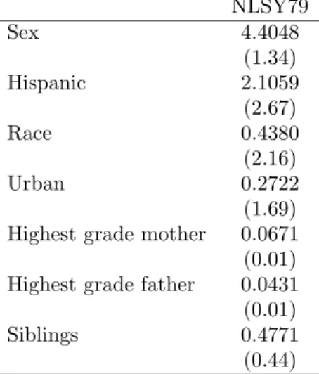
Estimated effects on college participation (selection equation used to implement the Heckman (1979) two-step procedure) are shown in Table 10.
NLSY79 Sex 4.4048 (1.34) Hispanic 2.1059 (2.67) Race 0.4380 (2.16) Urban 0.2722 (1.69) Highest grade mother 0.0671 (0.01) Highest grade father 0.0431 (0.01) Siblings 0.4771 (0.44)
Table 10: Estimated effects on college participation
The parameters estimated for the grant equation,g(Ωi) =α0+α1xi+α2yi+θXi+αλλbi+εi are reported
in Table 2
Wage estimation from the data proceed as follows: I first estimate a wage profile along the life-cycle. I impose rational expectations over the wage structure, i.e., agents can observe the wage profile along the life-cycle for each educational level and ability level. I control for experience and ability and perform estimations for each educational level. The wage equation is estimated for the first cohort using NLSY79 data available for the 1979 - 2006 period. The wage specification is: weduc
it =λ0+λ1expit+λ2expit2 +λ3xi+λ4Xi+εit.
This equation represents the log-wage structure for an individualiin periodtwho has an educational level
educ. The variable exp corresponds to experience and variable x to ability level. Xi is a set of controls
for individual and family characteristics. In these estimations I use information on white males only, whose annual wages are between $3,000 and $280,000. In the sample I include only individuals who participate in the labor force and are not attending school at that time. Estimates are presented in the Table 11.
Standard errors are in parenthesis. I project a hump shaped wage profile and estimate the average wage along the life-cycle. Average wages are reported in table 12.
D
Model Predictions
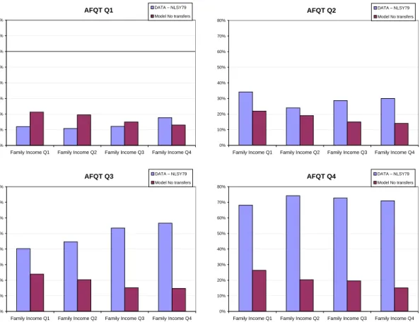
First, I solve the model without considering college utility. The model is employed to generate college attendance rates for each ability and family income group using parameters I estimated from NLSY79. These simulated outcomes are compared to those observed in the data. This exercise allows me to evaluate the performance of the model while only using parameters estimated from the data. Figure 4 presents the simulated and actual college attendance profiles of the NLSY79 cohort.
AFQT Q1 0% 10% 20% 30% 40% 50% 60% 70% 80%
Family Income Q1 Family Income Q2 Family Income Q3 Family Income Q4
DATA – NLSY79
Model No transfers AFQT Q2
0% 10% 20% 30% 40% 50% 60% 70% 80%
Family Income Q1 Family Income Q2 Family Income Q3 Family Income Q4
DATA – NLSY79 Model No transfers AFQT Q3 0% 10% 20% 30% 40% 50% 60% 70% 80%
Family Income Q1 Family Income Q2 Family Income Q3 Family Income Q4
DATA – NLSY79 Model No transfers AFQT Q4 0% 10% 20% 30% 40% 50% 60% 70% 80%
Family Income Q1 Family Income Q2 Family Income Q3 Family Income Q4
DATA – NLSY79 Model No transfers
Figure 4: College participation profile NLSY79-Data vs Model (no effor/cost utility parameter)
Adding the college utility parameters,φ(Ωj) =δ0+δ1xi+δ2yi, to the calibration of the model generates
High school College dropout College graduate λ0 9.046 9.071 9.344 (0.02) (0.04) (0.09) λ1 0.123 0.122 0.118 (0.004) (0.007) (0.012) λ2 -0.0027 -0.0026 -0.0027 (0.0001) (0.0002) (0.0004) λ3 0.157 0.037 0.186 (0.006) (0.012) (0.014)
Table 11: Estimated parameters for wage equations
college wage dropout wage non-college wage NLSY79 29,158 25,339 22,549
Table 12: Average wage per educational level, NLSY79 and NLSY97
Data Model Ability Family Income Q1 Q2 Q3 Q4 Q1 Q2 Q3 Q4 Q1 12.09% 34.19% 40.25% 68.15% 12.09% 33.03% 50.37% 68.14% Q2 10.83% 24.03% 44.65% 74.21% 13.12% 35.58% 51.00% 67.54% Q3 12.17% 28.66% 53.46% 72.73% 16.26% 35.01% 53.57% 68.81% Q4 17.72% 30.07% 56.60% 70.97% 17.70% 36.25% 56.77% 70.96%
Documentos de Trabajo
Banco Central de Chile
Working Papers
Central Bank of Chile
NÚMEROS ANTERIORES
PAST ISSUES
La serie de Documentos de Trabajo en versión PDF puede obtenerse gratis en la dirección electrónica:
www.bcentral.cl/esp/estpub/estudios/dtbc. Existe la posibilidad de solicitar una copia impresa con un costo de $500 si es dentro de Chile y US$12 si es para fuera de Chile. Las solicitudes se pueden hacer por fax: (56-2) 6702231 o a través de correo electrónico:[email protected].
Working Papers in PDF format can be downloaded free of charge from:
www.bcentral.cl/eng/stdpub/studies/workingpaper. Printed versions can be ordered individually for US$12 per copy (for orders inside Chile the charge is Ch$500.) Orders can be placed by fax: (56-2) 6702231 or e-mail: [email protected].
DTBC – 605
Determinants of Export Diversification Around The World: 1962 –
2000
Manuel R. Agosin, Roberto Álvarez y Claudio Bravo-Ortega
Enero 2011
DTBC – 604
A Solution to Fiscal Procyclicality: the Structural Budget
Institutions Pioneered by Chile
Jeffrey Frankel
Enero 2011
DTBC – 603
Eficiencia Bancaria en Chile: un Enfoque de Frontera de
Beneficios
José Luis Carreño, Gino Loyola y Yolanda Portilla
Diciembre 2010
DTBC – 602
Chile’s Structural Fiscal Surplus Rule: A Model – Based
Evaluation
Michael Kumhof y Douglas Laxton
Diciembre 2010
DTBC-601
Price Level Targeting and Inflation Targeting: a Review
Sofía Bauducco y Rodrigo Caputo
Diciembre 2010
DTBC-600
Vulnerability, Crisis and Debt Maturity: Do IMF Interventions
Shorten the Length of Borrowing?
DTBC-599
Is Previous Export Experience Important for New Exports?
Roberto Álvarez, Hasan Faruq y Ricardo A. López
Noviembre 2010
DTBC-598
Accounting for Changes in College Attendance Profile: A
Quantitative Life-cycle Analysis
Gonzalo Castex
Noviembre 2010
DTBC-597
Fluctuaciones del Tipo de Cambio Real y Transabilidad de Bienes
en el Comercio Bilateral Chile - Estados Unidos
Andrés Sagner
Octubre 2010
DTBC-596
Distribucion de Probabilidades Implicita en Opciones Financieras
Luis Ceballos
Octubre 2010
DTBC-595
Extracting GDP signals from the monthly indicator of economic
activity: Evidence from Chilean real-time data
Michael Pedersen
Octubre 2010
DTBC-594
Monetary Policy Under Financial Turbulence: An Overview
Luis Felipe Céspedes, Roberto Chang y Diego Saravia
Octubre 2010
DTBC-593
The Great Recession and the Great Depression: Reflections and
Lessons
Barry Eichengreen
Septiembre 2010
DTBC-592
Evidencia de Variabilidad en el Grado de Persistencia de la
Política Monetaria para Países con Metas de Inflación
Benjamín García
Septiembre 2010
DTBC-591
Mercados de Financiamiento a los Hogares en el Desarrollo de la
Crisis Financiera de 2008/2009
Gabriel Aparici y Fernando Sepúlveda