Consequences of Aid Volatility for Macroeconomic
Management and Aid Effectiveness
JOHN HUDSON
*University of Bath, UK
Summary.—We conclude that individual aid sector volatility matters as well as total aid volatility. Easily, the most important contrib-utor to total volatility is debt aid. The most volatile aid sectorsper seinclude debt, industry, and humanitarian, and the least include education and health. In several sectors volatility appears to have peaked around 2006. Within individual countries, sector volatility is often corrected for in the following period, there are also sometimes knock-on effects on other sectors. Finally we examine the impact of sector aid, and aid volatility, on school completion rates, death rates, Internet usage, and mobile phone subscriptions.
Ó2014 UNU-Wider. Published by Elsevier Ltd. This is an open access article under the CC BY license (http://creativecommons.org/licenses/ by/4.0/).
Key words— CRS data base, aid volatility, sector aid, school completion rates, Internet users
1. INTRODUCTION
In recent years the impact of aid has been more favorably viewed in the literature. One negative aspect, however, has been aid volatility. Celasun and Walliser (2008) argue that unexpected aid shortfalls can force governments to dispropor-tionately cut investment, including in human capital, while aid windfalls can disproportionately boost government consump-tion. The issue is relatively new to the literature.Pallage and Robe (2001)observed that aid is highly volatile with an aver-age volatility of about 25% in African recipients and 29.5% in nonAfrican recipients. But perhaps it was the work of Bulı´rˇ and Hamann (2003, 2008) which had most early influence. They argued that the volatility of aid is (i) greater than that of government revenue, (ii) increasing over time, and (iii) pro-cyclical (i.e., aid flows are inversely correlated with the level of government expenditures). Others have since built on and modified their conclusions. For example,Hudson and Mosley (2008a)find that volatility as a whole reduces growth given the level of aid, but not in a uniform way, differentiating between upside and downside volatility.
The majority of this work focuses on the totality of aid and its impact on key macroeconomic variables such as growth and government expenditure. Indeed this is also the case with the impact of aid itself. This is problematic. Why should health aid promote growth as equally as infrastructure aid, or vice versa with respect to targets such as infant mortality? Why, too, should volatility in these two sectors have the same impact? In this paper we seek to examine the nature of aid vol-atility as it relates to specific aid sectors. The database we use is the OECD’s Creditor Reporting System (CRS) on the DAC website. This gives detailed information on aid disbursements, and, over a longer time, commitments, by 50 different sectors and subsectors. The data on the former are only available in a reliable form since 2002, but on a panel data basis this is now sufficient to allow meaningful analysis.
We are also interested in analyzing the impact of aid and aid volatility on specific, and in some cases fairly narrow, targets. Much of aid works not so much on the macroeconomy, although there may, for example, be exchange rate effects and policy environment effects for all aid, but rather on indi-vidual aspects of the economy. The road built between A and B facilitates trade between those two locations, a new
hos-pital in location C facilitates healthcare in that location. Aid and aid volatility then impact on those projects, and, spillover effects apart, not on others. Now if there is a temporary switch in aid from healthcare to secondary education, this will not show up in the overall aid figures as volatility. The two will cancel each other out. But the healthcare project will have suf-fered from negative volatility and the education project from positive volatility. Hence a knowledge and understanding of aid sector volatility is important.
The paper proceeds as follows. In the next section, we review the literature, after which we discuss methodological and theoretical issues. Section 4 introduces the data. The empirical analysis follows. In this, we first decompose overall volatility into its constituent, sector parts. We then analyze the extent to which volatility is a dynamic process. Finally we examine the impact of the different aid sectors and associated volatility, on selected “micro targets,” i.e., death rates, pri-mary school completion rates, Internet usage, and mobile phone subscriptions. We then conclude the paper.
Table 1defines some key concepts and the measures of vol-atility we make use of in this paper. We use several different measures of volatility as is appropriate to the purpose for which it is being used. But, as is clear from the table, they are all based on the same basic variable, the error term from a trend regression.
2. LITERATURE REVIEW (a)Measuring aid volatility
The key initial work in this area is byBulı´rˇ and Hamann (2003, 2008). Their empirical work (ibid. 2008) is based on a
* This study paper has been prepared within the UNU-WIDER project
“Foreign Aid: Research and Communication (ReCom)” directed by T-ony Addison and Finn Tarp, and supported by specific contributions from the governments of Denmark (Ministry of Foreign Affairs, Danida) and Sweden (Swedish International Development Cooperation Agency— Sida). I would like to acknowledge their help and also the extraordinarily detailed and helpful comments of several anonymous referees. Final revision accepted: December 21, 2013.
0305-750X/Ó2014 UNU-Wider. Published by Elsevier Ltd. This is an open access article under the CC BY license (http:// creativecommons.org/licenses/by/4.0/). www.elsevier.com/locate/worlddev
http://dx.doi.org/10.1016/j.worlddev.2013.12.010
sample of 76 countries from 1975 to 2003. They use a Hodrick–Prescott filter1to derive aid residuals from a trend. The square of those residuals then measure volatility in a specific year for an individual country. Critical in all this is how one scales aid, particularly when comparing volatilities between different variables. Bulı´rˇ and Hamann specify aid in US dollars and government revenue in domestic currency. Both series were transformed into proportions of nominal GDP, PPP GDP, and constant US dollars per capita. This was done in part to remove the impact of scale on variabil-ity––clearly a variable with a large mean will tend to have a large variance. But when this is done, the resultant ratio is affected by both the variance of GDP, the variance of the rev-enue variable, e.g., aid, and the covariance between the two. The normalization process thatHudson and Mosley (2008a) employed involved defining all variables as a proportion of their mean value for the whole estimation period.
In their original paper, Bulı´rˇ and Hamann found that vola-tility was highest in the countries which are most aid-depen-dent, which are generally the poorest and most vulnerable. However, in their 2008 paper, they found that the pattern to be more complex, and that both those countries that are little dependent on aid and those that are heavily dependent on aid display high aid volatility relative to government revenue. Hudson and Mosley (2008a)in a subsequent paper found no evidence for highly aid dependent countries to have higher vol-atility. Indeed, they concluded that volatility declines as the aid-revenue ratio increases. But to a large extent they were able to confirm many of the conclusions of Bulı´rˇ and Hamann, for example that the ratio of aid to government revenue vola-tility was in excess of one for almost all countries. The volatil-ity of overseas aid was also noted to be severe, in relation to the volatility of domestic revenue, and increasing over time.
(b)The causes and the macroeconomic impact of aid volatility
Relatively little work has been done in analyzing the causes of volatility and how to reduce it. However, in a work which par-allels that ofFielding and Mavrotas (2005), Hudson and Mosley (2008a)examined the link between volatility and donor concen-tration. There was a tendency for countries with high two-donor concentration ratios, i.e., the share of aid provided by the two biggest donors, to have relatively high volatility. They also
found that in part, volatility was in response to recipient need, e.g., the famines in Ethiopia, but in part it was impacted on by donor coordination. Eifert and Gelb (2008) argued that the costs of aid volatility can be dramatically reduced by a flexible pre-commitment rule which adjusts aid flows in response to improvements or deteriorations in country performance rat-ings. They also suggested that a buffer stock of annual aid-financed spending might enable a corrective feedback loop, with the buffer depending on the size and variability of aid flows. Turning to self-insurance by recipient countries,Agenor and Aizenman (2010)studied the impact of aid volatility in a two-period model, with a first-two-period contingency fund financed through taxation. Unsurprisingly, an increase in aid volatility is shown to raise the optimal contingency fund. But if future aid also depends on the size of the contingency fund, the optimal recipient policy may entail no self-insurance.
Much more work has focused on the impact of volatility on
the macroeconomy. For example, Lensink and Morrissey
(2000)concluded that volatility damages the macroeconomic effectiveness of aid. Arellano, Bulı´rˇ, Lane, and Lipschitz (2009) examined the effects of aid and its volatility on con-sumption, investment, and the structure of production in the context of an inter-temporal, two-sector general equilibrium model. They argued that a permanent flow of aid mainly finances consumption rather than investment and that aid vol-atility results in substantial welfare losses to consumers, equiv-alent to 8% of the aid budget. Hudson and Mosley (2008b) analyzed the impact of aid volatility on GDP/GNP shares of expenditure. Negative volatility reduces investment and gov-ernment expenditure shares and also the import share. This may be because of the type of aid which is subject to volatility, or because consumers are better able to absorb shocks by drawing on savings and/or borrowing than other agents. The results also suggest a limited ability of governments to rearrange revenue flows to reduce the impact of volatility upon their expenditure priorities. Positive volatility also reduces investment and government expenditure shares, as well as increasing consumers’ expenditure share. These results suggest that absorptive capacity constraints particularly limit aid’s effectiveness with respect to both investment and government spending.Rodrik (1990) also analyzed the problems revenue volatility can cause developing countries, while Mosley and Suleiman (2007)showed that the ability of the recipient coun-Table 1. Key Definitions and Measures of Volatility
Aid sector This is the sector, or subsector, at which the aid is identified. Examples include health and program assistance. The term“sector”is the one employed on the CRS database. The different aid sectors we use are defined in theAppendix Table. They are chosen to be a comprehensive summary of total aid and also to reflect important social and productive sectors
Aid target This is the specific identifiable variable on which the aid is designed to impact. It could be literacy rates, Internet usage, or at a local level, access to safe drinking water in a specific location
Measures of volatility
Aid volatility (Table 2) This represents the mean of the square of the error term from regressing aid disbursements on a trend and trend squared for each country. If predicted aid from this regression is negative, then a lower bound of zero is imposed and the error adjusted accordingly.
Mean adjusted CV of aid volatility (Table 2)
Mean adjusted CV (coefficient of variation) divides the standard error of aid volatility, as defined above, in each year by the mean value of aid in all years for each country. In some years, particularly for debt aid, disbursements are low, which would lead to very large CVs as normally calculated
The aid error term (Tables 3 and 4)
InTable 3we represent the results of an“asymmetric VAR”based on the error term from the trend regression described above. This error term when squared is aid volatility, but is in its original form, more suitable for analysis in a VAR. This is also the basis for the positive and negative error terms used inTable 4as described in the Table The volatility measure
Figures 1 and 2)
InFigures 1 and 2the square root of aid volatility, as defined forTable 2, is regressed on a time trend and trend squared to fit trends in volatility. The square root was used as this more closely relates to the error itself and is less affected by outliers
try’s public sector to implement coherent investment programs and fiscal policies is reduced by aid volatility.
Chauvet and Guillaumont (2009) concluded that aid tends to neutralize volatility in export flows and also income volatil-ity, while aid volatility reduces its effectiveness in these respects. They also showed that the higher effectiveness of aid in vulnerable countries is, to a large extent, due to this sta-bilizing effect. Hudson and Mosley (2008a) differentiated between positive/upside and negative/downside volatility. Both reduce the impact of aid on growth, but subsequently some of this adverse impact is reversed, although only for positive volatility. With negative volatility there is no such reversal. This may reflect problems of absorptive capacity being short-term only. Positive volatility may also be reacting to emergencies and reflect an element of flexibility inherent in “reactive”forms of aid. The high incidence of this type of aid is, therefore, potentially an asset rather than a liability. Even negative volatility might feasibly have longer-term beneficial impacts, in persuading recipients to move toward policy reform, which are not apparent within the relatively short time-horizon Hudson and Mosley analyzed.
(c)A more disaggregated approach to the impact of aid volatility
Some studies have examined other macroeconomic factors such as public sector behavior in developing countries ( Mav-rotas & Ouattara, 2006a, 2006b). But there have been few attempts to focus the attention more finely, and there is also a tendency to treat all aid as the same. Clemens, Radelet, and Bhavnani (2004)questioned this and argued that different types of aid, impact on growth over different time frames, and to lump it all together in cross-country growth regressions is inappropriate. They focused on aid which could stimulate growth in a four year time-horizon. This includes budget and balance-of-payments support, investments in infrastruc-ture, and aid for productive sectors such as agriculture and industry.
Fielding and Mavrotas (2005)distinguished between sector aid and total aid in examining aid volatility in 66 countries over 1975–2004. They built on the conclusion by Levin and Dollar (2005)that aid is more volatile in countries identified as having weak political institutions and historically poor macroeconomic policies. Consistent with this, Fielding and Mavrotas (2008)concluded that institutional quality and mac-roeconomic stability affect aid volatility, as does reliance on a small number of donors. However, the relative importance of these effects varies across different aid types. Reflecting this, countries that have recently agreed to International Monetary Fund (IMF) conditionality experience higher total aid volatil-ity, but not higher sector aid volatility. This suggests that hav-ing agreed to such conditionality is a sign of weakness in existing macroeconomic policy. They also found that the fac-tors driving up sector aid volatility are different to those impacting on total aid volatility. In addition, a number of indi-vidual donors (in particular, Germany, US and the European Commission) appear to be associated with relatively high vol-atility sector aid flows.
The possibility that different types of aid may have different impacts on the recipient has been noted by, e.g.,Chatterjee, Sakoulis, and Turnovsky (2003), Clemenset al.(2004), Reddy and Minoiu (2006), Mavrotas (2002, 2005)andMavrotas and Ouattara (2006a). Mavrotas and Ouattara (2007)found that both project aid and financial program aid exert a positive, sig-nificant effect on total expenditure, but that project aid also appears to increase capital expenditure, while financial
program aid is associated with an increase in government con-sumption. This suggests that project financing is more likely to be growth enhancing than program aid. They found no evi-dence that aid flows are associated with a reduction in taxation effort. Indeed, project aid flows are associated with an increase in trade tax.Neanidis and Varvarigos (2009), using the CRS database, found that aid disbursements used for productive sectors have a positive effect on growth, but pure transfers reduce growth. Aid volatility is found to hurt growth, only when aid is used productively, while the volatility of pure aid disbursements is associated with higher growth.
Wolf (2007)andStuckler, Basu, and McKee (2011)focused on the effects of aid volatility on micro-targets. Wolf analyzes the effects of the volume and volatility of aid on education, health, water, and sanitation outcomes. Overall the share of official development assistance (ODA) that is provided for education and health seems to have a positive impact on out-comes in these sectors, whereas total aid seems to be negatively associated with these. Aid volatility is associated with better outcomesin sanitation, water, and infant mortality, contrary to expectations. The merits of this paper are in its focus and the use of sector aid as well as total aid. But the research mea-sures aid volatility as the coefficient of variation for total aid during 1980–2002, while the regressions themselves relate to just 2002. Hence, this is entirely different to the concept of vol-atility as used by most of the literature, and it is not really clear what this is picking up. Stuckler, Basu, and McKee focus on one of the possible consequences of volatility. They find that for each $1 of development assistance for health, about $0.37 is added to the health system. However, evaluating IMF-borrowing versus nonIMF-borrowing countries reveals that nonborrowers add about $0.45, whereas borrowers add less than $0.01 to the health system. This, they argue, could be because World Bank and IMF macroeconomic policies spe-cifically encourage governments to divert aid to reserves to cope with aid volatility.
There are thus arguably gaps in the literature, which we seek to reduce, in (i) understanding the interrelationship between volatility of the different aid sectors, on which there has been very little work and (ii) understanding the impact of sector aid, and aid volatility, on micro targets. In this respect, the key part of the paper is Section5. We begin by looking at volatility and trends in volatility of total aid and its constituent parts. This will help us understand what contributes most to the vol-atility of total aid and whether volvol-atility is increasing or decreasing. We then turn to analyze the interactions between the different aid sectors through an “asymmetric vector autoregression (VAR)”, before finally turning to analyze the impact of sector aid and aid volatility on five specific targets.
3. THEORY AND METHODOLOGY (a)The micro–macro adding up problem
Aid can impact on the target variables in two different ways, which one might loosely term supply side and demand side effects. Take, e.g., school completion rates which we examine later. Education aid targets the supply side, potentially improving the educational system, by, e.g., increasing the number, or the quality, of schools. Other types of aid can loosen the constraints on children going to school. For exam-ple, health aid, if it increases the health of the adult popula-tion, potentially increases their earning power and their ability to contribute to the household production function, reducing the need to rely on children in these respects, thus
raising the “demand” for education. Supply side effects can also occur through aid which increases access to the Internet. Hence it is not simply a case that if we wish to target human capital we should think exclusively about education aid.
The total impact of aid from all sectorsj(Aj) on a particular target (Yi) can be written as:
XJ j¼1 Aj @Yi @Aj ð1Þ
For many aid sectors and targets, the partial derivative will be zero. We would expect education aid to impact on primary school completion rates, rather than energy sector aid. But, as already argued, primary school completion rates may also depend upon socioeconomic factors and hence other aid sec-tors may be relevant in this context. The total impact on some macroeconomic variable such as growth (g) will then be found by summing the impact across the I targets:
XJ j¼1 XI i¼1 Aj @g @Yi @Yi @Aj : ð2Þ
Aid volatility impacts upon this by adversely impacting upon
oYi/oAj, i.e., reducing the effectiveness of aid. The total impact of aid volatility on the macroeconomic target will then equal XJ j¼1 XI i¼1 Aj @g @Yi AVj @Yji @AV j : ð3Þ
whereAVj is the volatility of AjandY j
i¼
@Yi
@Aj. As we shall see
later, there is an argument that we should further distinguish between positive and negative aid volatility.
Simply focusing on the impact of total aid volatility on a sin-gle macroeconomic variable such as growth misses two differ-ent effects. First, aid in sectorjmay switch between (micro-) targets, that is, education aid, for example, switches from one locality to another. This will not be reflected in overall aid volatility, but will result in positive volatility for one (micro-) target and negative volatility for another one. Second, and more the concern of this paper, aid may switch between sectors. Again, overall aid will show no volatility, but the indi-vidual sectors, will be affected.
(b)The donor’s allocation problem
We assume donors tend to maximize some form of welfare function subject to a budget constraint. They will be aware that volatility is potentially damaging to both the recipient country and its own credibility as a donor. But nonetheless, aid may still be volatile for a number of reasons. First, volatil-ity may be a response to recipient behavior. A failure to
imple-ment previous commitments, or a perceived corrupt
bureaucracy or political system, may see aid fall below intended disbursements. In this case we would expect to see no recovery of aid in succeeding periods, following a shortfall. Indeed the reverse may be the case, shocks may be perpetu-ated. Alternatively, an emergency in one country may lead to a tightening of budgets for other countries. In this case the donor will juggle the aid budget as best they can. Within a country, they will reduce the aid most in those sectors which are least important to the donor2and where, for example, it can be substituted between t and t+ 1 with relatively little adverse impact. Similarly there may be a need to switch aid between sectors within countries, quite independently of what is happening elsewhere. This can occur in response to an emer-gency in the country or unforeseen developments possibly
associated with existing aid spending. In this case the donor may seek to reduce aid in related sectors, e.g., given a surge in program aid, reduce government aid. However, as already indicated, having diverted aid away from sectorjin periodt, the donor may respond by increasing it above trend in the fol-lowing period and vice versa in a sector which saw an aid surge. In this way aid shocks can have ripple effects.
(c)Measuring volatility
We do not use the Hodrick–Prescott filter to derive esti-mates of volatility, as, particularly with respect to disburse-ments, we have relatively few data points to work with for each country.3 Instead we regress aid in sector j on a time trend and its square to calculate the trend. Squared deviations from this trend are then assumed to represent volatility. This leaves the possibility that some predicted aid values may be negative; we therefore impose a lower bound of zero and adjust the measures of volatility accordingly.4 Each trend is fitted for one country at a time. This assumes that in the initial periods, recipient countries are aware of this trend; that if aid, for example, rises steadily over the period, they are aware of this right at the beginning of the period. It is not obvious this is the case, and certainly at the beginning of a sustained period of growth, or decline, in the aid budget, the recipient country may be surprised. Even if the change is anticipated, they may well have difficulties in responding to change, or harbor doubts as to whether donors will fulfill commitments.
4. DATA
The CRS has annual data on aid, relating to commitments and disbursements. Commitments are in effect promises of aid, which may be fulfilled immediately, in the future or even not at all. Disbursements are the “release of funds to or the purchase of goods or services for a recipient. They record the actual international transfer of financial resources, or of goods or services valued at the cost to the donor”. The CRS has been used in many of the recent analyses on aid volatility and aid impact (e.g.,Clemenset al., 2004; Fielding & Mavro-tas, 2008; Neanidis & Varvarigos, 2009). But there are doubts about its suitability in early years. With respect to disburse-ments, before 2002 the annual coverage was below 60%, while it has been around and over 90% since 2002, and reached nearly 100% by 2007. Thus the OECD warns against using the earlier data for sectors, and these data on the main data-base are available only since 1995 for commitments and since 2002 for disbursements. As a consequence, 2002 represents the start date for the sample period we use in this paper. In our main regression analysis, as in the next sector, there are 137 countries. The panel is almost balanced with just two countries having less than the full number of observations.
The term “aid sector”signifies the sector of the recipient’s economy that the aid activity is designed to assist, e.g., health, energy, or agriculture. Some contributions are not targeted to a specific sector, e.g., emergency aid. These are called“ nonsec-tor allocable aid.”But all the data are derived from the section of the database termed“sector,”which is why we use this gen-eric term in this paper. For activities cutting across several
sec-tors, either a multi-sector sector code or the code
corresponding to the largest component of the activity is used. We analyze all the main sectors, or their constituent parts, but not all of the subsectors. Instead we focus on the social and production subsectors. More details on the data can be found in anAppendix.
In order to be able to combine data from different countries, we need to normalize aid in some manner. We do this by tak-ing aid as a proportion of recipient country GDP. The pros and cons of the various alternatives are discussed inHudson and Mosley (2008a). We are focused on comparing aid volatil-ity between different aid sectors rather than between aid and some other revenue variable such as government expenditure. In this case, in relative terms, the various differences between different normalization procedures are less important. We focus our analysis on disbursements rather than commitments, as these represent actual aid flows rather than the promises of flows. The data are available for different donors and groups of donors. We use ODA for all donors.
5. RESULTS
In this section we seek to (i) analyze the volatility of individ-ual sectors, (ii) identify any trends, albeit over a very short time period, (iii) analyze the extent to which aid shocks are corrected for in the following year and (iv) analyze the extent to which different aid sectors impact on different target vari-ables.
(a)The makeup of overall volatility
We begin by examining the causes of volatility, in terms of linking overall volatility to its component parts. As Fielding and Mavrotas (2008) emphasize, the variance of a variable made of n components is the sum of thenvariances plus twice each of the covariances. Thus the overall variance can exceed or fall short of the sum of each of the components, or sector, variances depending upon the signs of the covariances. If over-all, the covariances are positive, it will indicate that the sectors have tended to move together, with aid tending to increase or decrease for countries as a share of GDP. If on balance they are negative, it will indicate that there have been shifts in aid between sectors within countries.
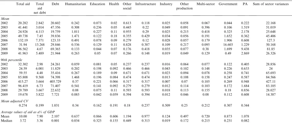
Table 2 shows the volatility of total disbursements in the first column, reporting the mean and the 90th percentile. It will be recalled that these relate to the squared residuals from a trend based regression.5 In the following columns we have the same data for most individual sectors. The final column relates to the sum of all the sector volatilities, not just the ones in this table. There are substantial differences between the first and the final columns, but, as expected, the correlation between the two is very high. Hence in an OLS regression of total aid volatility on summed sector volatility across all years and countries, theR2is 0.89. The difference between the two is due to the covariances between the different sectors impacting on total aid volatility in the first column but not the final one.6 It is not a simple story of one being consistently greater than the other, indicating that in some years the net effect of the covariances is negative and in others it is positive. Thus in 2007 there were 12 significant, at the 1% level, negative aid sec-tor correlations and eight positive ones, whereas in 2009 these figures were five and 11 respectively. There is, however, a ten-dency, 2007 apart, for the positive correlation to become rela-tively more important over time, as reflected in the gap between the first and final columns becoming steadily more positive. This suggests that increasingly all aid sectors within countries are moving up or down together, and that trade-offs within countries are becoming relatively less important. It is a moot question as to which is the better indicator of aid vola-tility, that relating to total aid or that to the sum of its constit-uent parts. However, as already indicated, it seems reasonable
to argue that it is more the latter, as the damage done to health, education and industry is not reduced (increased) because they are negatively (positively) correlated with each other. If this is accepted, then it follows that a measure of aid volatility based on total aid is limited. Indeed arguably the problem is worse than this, as a single sector in itself is likely to be made of multiple subsectors, for example, in differ-ent localities.7This is related to the point made by Fielding and Mavrotas (2008)that an increase in sector aid volatility does not on average appear to entail any significant increase in total aid volatility. They go on to emphasize that, in general, the factors driving up sector aid volatility are not the same as those driving up total aid volatility.
The remaining columns relate to individual sector volatility. The most important sectors in explaining total volatility are debt aid followed by government and program assistance (PA) aid. Debt volatility in particular goes a long way to explaining total volatility. Take this out of the picture, as in the second column, and aid disbursements appear substan-tially less volatile. However, being averages the figures are mis-leading to an extent, as they are substantially affected by outliers. This is reflected in the figures for the 90th percentile. The peak year for total volatility as measured by the mean is 2006, followed by 2008. But for the 90th percentile, it is the cluster of years 2005–2007. The dominant factor in both 2006 and 2008 is the volatility of debt aid. However in 2007 aid to government also showed considerable volatility. As dis-cussed below, this may anticipate the peak in debt aid in the following year.
These data tell us the most important sectors in determining overall volatility, but do not tell us which sectors are most vol-atile. A sector may have a small entry in Table 2 simply because it is a small sector in absolute terms, but it may still in itself be characterized by high volatility. To analyze this, we need to remove the scale factor. Dividing the square root of the error squared term8 for aid sector A by the average level of A’s aid over all years, in a manner similar to the coef-ficient of variation, achieves this. The result is shown in the final row ofTable 2. We now get a very different picture. Debt aid is still the most volatile. But aid for the social sectors, including education and health, tends to exhibit low volatility. Apart from debt aid, the most volatile sectors are industry, PA, and government aid. There are significant correlations between sectors, which change from year to year. But over the whole period, there are five significant negative correla-tions where the absolute value for the correlation statistic exceeds 0.2. Three of these involved PA. This is consistent with our a priori beliefs regarding the likelihood of PA being prone to short-term aid switching. Based on similar criteria, there were also five positive correlations, three of which involved linkages between education, health, and multi-sector aid.9
(b)Trends in volatility
In this section we examine whether there are any trends in volatility. There has, as we saw in the literature review, been a lot of work done which has concluded that volatility has been increasing. There are two questions we seek to answer. Firstly, given this more recent data is it still increasing and sec-ondly, is the same pattern in evidence for all sectors? On the first of these, there is reason to suppose that the increase in volatility will have stopped and may even have been reversed. This is because of the publicity given to this issue both in pub-lic pronouncements and through the research work we have already reviewed. Policy makers will be aware of this and can be expected to respond accordingly. On the second issue,
Table 2. Volatility: Aid Disbursements, 2002–09
Total aid Total aid net debt
Debt Humanitarian Education Health Other social
Infrastructure Industry Other production
Multi-sector Government PA Sum of sector variances
Mean 2002 20.282 2.842 20.602 0.242 0.073 0.02 0.613 0.118 0.025 0.058 0.067 0.044 0.222 22.168 2003 41.441 3.014 47.356 0.308 0.236 0.05 0.445 0.22 0.049 0.091 0.396 0.106 1.519 51.019 2004 24.926 4.113 19.759 1.011 0.227 0.11 0.955 0.29 0.025 0.215 0.418 0.325 2.178 25.648 2005 49.738 7.45 39.836 1.471 0.122 0.18 0.355 0.429 0.034 0.056 0.191 1.652 0.362 45.406 2006 132.19 7.371 123.33 0.491 0.078 0.09 0.279 0.12 0.028 0.057 0.179 1.906 0.608 127.3 2007 31.94 13.268 29.846 0.536 0.129 0.11 0.828 0.387 0.109 0.217 0.095 16.603 1.229 50.168 2008 96.562 4.67 69.365 0.133 0.044 0.07 0.176 0.418 0.035 0.077 0.38 1.699 9.438 81.85 2009 41.963 5.489 21.944 0.263 0.05 0.07 0.266 0.148 0.019 0.049 0.129 0.49 2.869 26.326 90th percentile 2002 32.302 2.98 24.261 0.059 0.081 0.05 0.237 0.237 0.016 0.064 0.077 0.122 0.405 28.856 2003 24.59 6.001 11.829 0.202 0.198 0.092 0.466 0.466 0.043 0.102 0.148 0.226 0.633 24 2004 59.55 4.48 35.416 0.267 0.189 0.09 0.671 0.671 0.023 0.094 0.078 0.258 0.741 65.693 2005 85.808 9.568 74.398 1.468 0.196 0.084 0.474 0.474 0.013 0.108 0.158 0.247 0.587 84.566 2006 415.27 3.664 405.729 0.37 0.221 0.066 0.317 0.317 0.007 0.07 0.105 0.269 0.948 427.11 2007 96.419 6.73 71.407 0.541 0.141 0.092 0.279 0.279 0.012 0.114 0.103 0.172 1.684 83.105 2008 29.789 3.667 22.632 0.08 0.075 0.11 0.593 0.593 0.018 0.113 0.155 0.18 0.856 28.027 2009 19.678 3.822 7.721 0.085 0.042 0.059 0.394 0.394 0.012 0.046 0.08 0.112 0.608 14.387 Mean adjusted CV 0.274 0.199 1.031 0.34 0.162 0.191 0.18 0.237 0.509 0.25 0.212 0.307 0.344
Average values of aid as a% of GDP
Mean 10.00 7.90 2.107 0.637 0.866 0.606 1.194 0.977 0.124 0.497 0.720 0.873 1.078 Median 3.72 3.36 0.001 0.034 0.325 0.155 0.449 0.313 0.019 0.172 0.215 0.231 0.082
Notes:The figures relate to the mean and 90th percentile values across all years, and aid recipients, of aid volatility as defined inTable 1for the sectors defined in theAppendix. PA denotes program
assistance. The final column relates to the sum of volatility in all the individual aid sectors. This includes smaller sectors such as relating to refugees and administration which are not included in the previous columns. The mean adjusted CV adjusts volatility for the scale factor as described inTable 1.
CONSEQUE NCES OF AID VOLAT ILITY FOR MACRO ECONOMIC MANAGEM ENT AND AID EFFECTIVE NESS 67
we anticipate that there will be significant differences between sectors. Some may be deemed of particular importance, e.g., health and education which are at the heart of the Millennium Development Goals, and hence have not seen the same rise in volatility as others. For other sectors there may be external factors driving increased volatility, e.g., with respect to humanitarian aid, the increased frequency of natural disasters (Hudson & Mosley, 2008a).
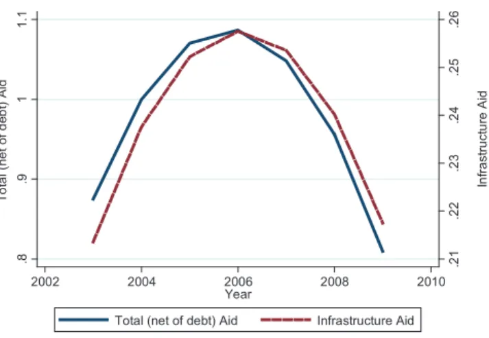
The measure of aid volatility frequently used tends to be the error term squared as reported inTable 2. In this analysis we will however not use this, but its square root,10which is less influenced by outliers. We regress this on a trend and squared trend, and use the coefficients to calculate a nonlinear trend. Country fixed effects are included to allow for systematic country differences. The curves for total aid, with debt netted out, and infrastructure, are shown inFigure 1. The trend vari-ables are jointly significant at the 5% level. We can see volatil-ity appears to increase until about 2006 after which it begins to decline. This nonlinear pattern, although not necessarily with the same turning point, is repeated for education and human-itarian aid, as can be seen fromFigure 2, and also for health and debt. The trend variables were jointly significant at the 1% level in all these equations. The turning point was 2006 for all apart for education and infrastructure, when it was 2005 and 2007 respectively. However, there were no significant trends, either linear or nonlinear, in government, PA, industry,
other-production, multi-sector aid, and other-social aid. We noted earlier that 2006 was a peak year for debt aid volatility and it is possible that this had knock-on effects on other aid sectors. This is not something we explore in more depth than in the VAR regressions which follow in the next section. Nor do we have a long enough run of data to discern any more general trends. But certainly there is no evidence that aid vol-atility is increasing.
(c)The dynamics of aid volatility
In this section we examine the dynamics of aid volatility via a modified VAR on aid volatility with respect to disburse-ments. Underlying these regressions is the behavior of donors trying to allocate aid to maximize its impact, given an objec-tive function as discussed earlier In any one period donors may be forced to reduce aid below trend, they will tend to do this in those sectors where it will do least harm, and in order to minimize the harm then to compensate for that short-fall in the following year. Some of these shocks may take the form of an aid surge in some other country or in some other sector within the same country. In order to be able to compen-sate for a sector shortfall the following year, within a budget which is approximately fixed over a several year period, the sectors which experienced the aid surge may see a reduction in aid. Of course an aid shortfall may reflect a punishment in some form by the donor on the recipient country, possibly in response to the failure to meet commitments previously made for aid given conditionally. In this case the shortfall would not be made good the following year, but could poten-tially be continued. There is also the possibility that aid surges will be corrected for.
We do not regress volatility on lagged volatility as in a stan-dard VAR, but in what we term an asymmetric VAR, distin-guishing between positive and negative volatility; that is, we regress the error term, rather than the error term squared, on lagged positive and negative errors terms11as two separate variables. As discussed above, positive and negative aid vola-tility are separate concepts, with separate causes and impacts. Thus there is reason to anticipate that they will have different impacts on future volatility within a VAR structure. If their coefficients are the same, then it is equivalent to a standard VAR. But our null hypothesis is that the impacts will be differ-ent. A second hypothesis is that the coefficients on a variable’s own lags will tend to be negative, e.g., that a shortfall in one year will be partially compensated for the following year. The specification of the variables in this VAR comprises all the sectors reported inTable 2. We have only a limited time dimension, but the cross-section element gives a reasonable number of observations. However, because of this we utilize only a first order VAR.
The coefficients on the other lagged variables will reflect the lagged trade-offs donors make in the aid allocation process. A negative coefficient indicates that an aid surge/fall in one sec-tor is subsequently being compensated for by a fall/surge in another sector. A positive coefficient may indicate closely related sectors where an increase in one signals a subsequent increase in another, possibly because aid in the first sector facilitates the subsequent increase of aid in the second. A pri-ori we expect there to be more negative interactions between related sectors, as donors seek to trade-off of“like with like.” The two government linked sectors, PA and Government, are obvious potential examples. Secondly we expect over-arching sectors to be particularly sensitive to shocks in other sectors, simply because they are closely related to many sectors. A key over-arching sector is PA. Finally, we anticipate that
.0 8 .1 .1 2 .1 4 .1 6 Ed u cat io n Ai d .1 .1 5 .2 .2 5 .3 H u ma n ita ri a n Ai d 2002 2004 2006 2008 2010 Year
Humanitarian Aid Education Aid
Note: See Table 1 and appendix for definitions
Figure 2. Trends in aid volatility.
.2 1 .2 2 .2 3 .2 4 .2 5 .2 6 In fr a str u ctu re A id .8 .9 1 1. 1 T o ta l ( n e t of d e b t) A id 2002 2004 2006 2008 2010 Year
Total (net of debt) Aid Infrastructure Aid
Note: See Table 1 and appendix for definitions
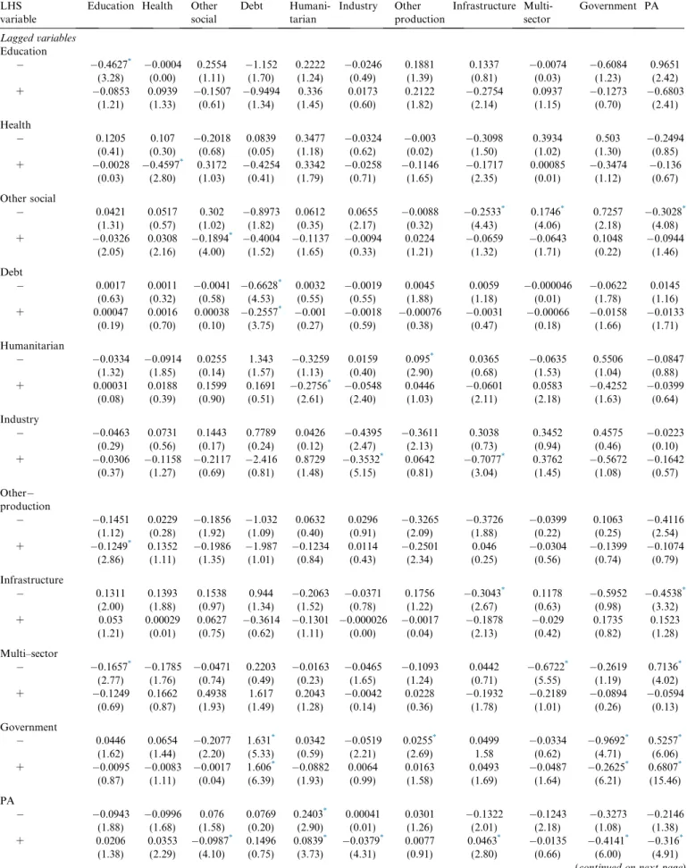
Table 3. Dynamic Impacts of Volatility
LHS variable
Education Health Other social Debt Humani-tarian Industry Other production Infrastructure Multi-sector Government PA Lagged variables Education 0.4627* 0.0004 0.2554 1.152 0.2222 0.0246 0.1881 0.1337 0.0074 0.6084 0.9651 (3.28) (0.00) (1.11) (1.70) (1.24) (0.49) (1.39) (0.81) (0.03) (1.23) (2.42) + 0.0853 0.0939 0.1507 0.9494 0.336 0.0173 0.2122 0.2754 0.0937 0.1273 0.6803 (1.21) (1.33) (0.61) (1.34) (1.45) (0.60) (1.82) (2.14) (1.15) (0.70) (2.41) Health 0.1205 0.107 0.2018 0.0839 0.3477 0.0324 0.003 0.3098 0.3934 0.503 0.2494 (0.41) (0.30) (0.68) (0.05) (1.18) (0.62) (0.02) (1.50) (1.02) (1.30) (0.85) + 0.0028 0.4597* 0.3172 0.4254 0.3342 0.0258 0.1146 0.1717 0.00085 0.3474 0.136 (0.03) (2.80) (1.03) (0.41) (1.79) (0.71) (1.65) (2.35) (0.01) (1.12) (0.67) Other social 0.0421 0.0517 0.302 0.8973 0.0612 0.0655 0.0088 0.2533* 0.1746* 0.7257 0.3028* (1.31) (0.57) (1.02) (1.82) (0.35) (2.17) (0.32) (4.43) (4.06) (2.18) (4.08) + 0.0326 0.0308 0.1894* 0.4004 0.1137 0.0094 0.0224 0.0659 0.0643 0.1048 0.0944 (2.05) (2.16) (4.00) (1.52) (1.65) (0.33) (1.21) (1.32) (1.71) (0.22) (1.46) Debt 0.0017 0.0011 0.0041 0.6628* 0.0032 0.0019 0.0045 0.0059 0.000046 0.0622 0.0145 (0.63) (0.32) (0.58) (4.53) (0.55) (0.55) (1.88) (1.18) (0.01) (1.78) (1.16) + 0.00047 0.0016 0.00038 0.2557* 0.001 0.0018 0.00076 0.0031 0.00066 0.0158 0.0133 (0.19) (0.70) (0.10) (3.75) (0.27) (0.59) (0.38) (0.47) (0.18) (1.66) (1.71) Humanitarian 0.0334 0.0914 0.0255 1.343 0.3259 0.0159 0.095* 0.0365 0.0635 0.5506 0.0847 (1.32) (1.85) (0.14) (1.57) (1.13) (0.40) (2.90) (0.68) (1.53) (1.04) (0.88) + 0.00031 0.0188 0.1599 0.1691 0.2756* 0.0548 0.0446 0.0601 0.0583 0.4252 0.0399 (0.08) (0.39) (0.90) (0.51) (2.61) (2.40) (1.03) (2.11) (2.18) (1.63) (0.64) Industry 0.0463 0.0731 0.1443 0.7789 0.0426 0.4395 0.3611 0.3038 0.3452 0.4575 0.0223 (0.29) (0.56) (0.17) (0.24) (0.12) (2.47) (2.13) (0.73) (0.94) (0.46) (0.10) + 0.0306 0.1158 0.2117 2.416 0.8729 0.3532* 0.0642 0.7077* 0.3762 0.5672 0.1642 (0.37) (1.27) (0.69) (0.81) (1.48) (5.15) (0.81) (3.04) (1.45) (1.08) (0.57) Other production 0.1451 0.0229 0.1856 1.032 0.0632 0.0296 0.3265 0.3726 0.0399 0.1063 0.4116 (1.12) (0.28) (1.92) (1.09) (0.40) (0.91) (2.09) (1.88) (0.22) (0.25) (2.54) + 0.1249* 0.1352 0.1986 1.987 0.1234 0.0114 0.2501 0.046 0.0304 0.1399 0.1074 (2.86) (1.11) (1.35) (1.01) (0.84) (0.43) (2.34) (0.25) (0.56) (0.74) (0.79) Infrastructure 0.1311 0.1393 0.1538 0.944 0.2063 0.0371 0.1756 0.3043* 0.1178 0.5952 0.4538* (2.00) (1.88) (0.97) (1.34) (1.52) (0.78) (1.22) (2.67) (0.63) (0.98) (3.32) + 0.053 0.00029 0.0627 0.3614 0.1301 0.000026 0.0017 0.1878 0.029 0.1735 0.1523 (1.21) (0.01) (0.75) (0.62) (1.11) (0.00) (0.04) (2.13) (0.42) (0.82) (1.28) Multi–sector 0.1657* 0.1785 0.0471 0.2203 0.0163 0.0465 0.1093 0.0442 0.6722* 0.2619 0.7136* (2.77) (1.76) (0.74) (0.49) (0.23) (1.65) (1.24) (0.71) (5.55) (1.19) (4.02) + 0.1249 0.1662 0.4938 1.617 0.2043 0.0042 0.0228 0.1932 0.2189 0.0894 0.0594 (0.69) (0.87) (1.93) (1.49) (1.28) (0.14) (0.36) (1.78) (1.01) (0.26) (0.13) Government 0.0446 0.0654 0.2077 1.631* 0.0342 0.0519 0.0255* 0.0499 0.0334 0.9692* 0.5257* (1.62) (1.44) (2.20) (5.33) (0.59) (2.21) (2.69) 1.58 (0.62) (4.71) (6.06) + 0.0095 0.0083 0.0017 1.606* 0.0882 0.0064 0.0163 0.0493 0.0487 0.2625* 0.6807* (0.87) (1.11) (0.04) (6.39) (1.93) (0.99) (1.58) (1.69) (1.64) (6.21) (15.46) PA 0.0943 0.0996 0.076 0.0769 0.2403* 0.00041 0.0301 0.1322 0.1243 0.3273 0.2146 (1.88) (1.68) (1.58) (0.20) (2.90) (0.01) (1.26) (2.01) (2.18) (1.08) (1.38) + 0.0206 0.0353 0.0987* 0.1496 0.0839* 0.0379* 0.0077 0.0463* 0.0135 0.4141* 0.316* (1.38) (2.29) (4.10) (0.75) (3.73) (4.31) (0.91) (2.80) (0.66) (6.00) (4.91)
(continued on next page)
health, being at the heart of the Millennium Development Goals, will tend to be protected from volatility, as suggested by its low volatility in Table 2. The same may also be true for education.
The results are shown in Table 3. We use as our bench-mark the 1% significance level. Focusing first on the own effects, i.e., the impacts of the twin lagged dependent vari-ables, there is a tendency for errors in period t1 to be partially corrected for in the following period. This is the case for five of the 12 negative volatilities and seven of the positive volatilities. There are no significant positive coefficients, indicating an absence of shock persistence. It is thus not simply a matter of volatility being limited to a single period and then a return to trend, it is that a positive injection of aid above trend tends to be partially compen-sated for in the following period by a below-trend level of aid and vice versa. There are also 21 cross-sector impacts and, as anticipated, over half relate to PA. In six cases a shock from PA has impacts on other sectors and in five cases the reverse is the case. When the impact is negative, the former is consistent with the hypothesis that other sec-tors are “paying for” the aid surge in PA. In two sectors there was a positive knock-on effect from positive volatility in PA, these were humanitarian aid and infrastructure aid. The latter may indicate the preparatory work that needs to take place before a large infrastructure project can begin. The former may relate to disaster prevention, which is part of humanitarian aid. Also in accordance with our expecta-tions, none of the interactions relate to health, although two do involve education. There is little evidence for debt aid crowding out other forms of aid.12 The only linkage to debt aid is from government sector aid, which is consis-tent with the donor preparing the recipient for subsequent debt relief as suggested by Cassimon and Essers (2013). Apart from PA, the other sectors which see substantial interaction are government and infrastructure aid, which to an extent share some of the over-arching characteristics of PA. For example, infrastructure aid declines in response to positive volatility in industry aid. These two sectors are competing for similar resources (Choi, 2005) and an increase in aid for one may signal a decline for the other.
Is the use of an asymmetric VAR justified? Just focusing on the own lagged impact, there is a significant difference in the two coefficients in one equation at the 1% level of nificance. It is, however, often more difficult to prove a sig-nificant difference between two variables than significance
per se, and two other equations have significantly different coefficients at the 5% level of significance and three at the 10% level. The use of an asymmetric VAR thus seems justi-fied.
(d)The impact of volatility
In this section we analyze the impact of volatility on several aspects of a country, which in general have not been the sub-ject of much research, at least with respect to the impact of aid. In part this is because some of the data, such as that relating to Internet usage, are available only over a limited time frame. But this time frame tends to match our data from the CRS database, and in any case with the cross-section data supple-menting the time series data, there are now sufficient observa-tions to make analysis plausible, even if slightly constrained. The other target variables are death rates, male and female pri-mary school completion rates and mobile phone subscriptions. In general these target variables tend to show substantial var-iation over time, albeit often along a trend. The choice of our variables is, in part, dictated by data availability and in part by the fact that they represent a combination of social targets and “economic targets.”
We argued earlier that aid can impact on target variables in two different ways, reflecting supply side and demand side effects. With respect to Internet usage, infrastructure aid may improve the quality and coverage of the Internet connec-tion, a supply side effect, but other aid such as for education and industry can increase the demand from users, either home users, or business ones. In terms of death rates, health aid can improve the quality of care, but aid which promotes growth can increase living standards and reduce poverty thus impact-ing on death rates, while education can facilitate healthy life styles. Hence when thinking about what types of aid might successfully promote a particular target, we should not restrict ourselves to the“obvious ones.”
Including aid in a regression with the target variable on the left hand side variable is not satisfactory as it will only capture a temporary impact and once the aid has finished, the target will return to the previous trend.13But the impact of aid on school completion rates should have a longer-term impact, whether that impact comes from supply side or demand side effects. Similarly if aid impacts on Internet usage, the impact is unlikely to be temporary, but longer lasting, as once some-one is a user, they will tend to stay a user. The same is true, to varying degrees, of the other variables we are analyzing, For this reason, we model these variables in a similar manner to the impact of aid on GDP or GDP per capita in growth regres-sions (Barro, 1991). Similar to the growth regressions, we include the base year value of the variable, e.g., for death rates, the death rate in the first year of our sample. The coefficient on this is expected to be negative, and if so will relate to the speed of convergence. We also include year dummy variables to cap-ture general movements over time caused, for example, by technical progress or the diffusion of a new technology. The Table 3—(continued)
LHS variable
Education Health Other social Debt Humani-tarian Industry Other production Infrastructure Multi-sector Government PA Asymmetry 5% ns 10% 5% ns ns 10% ns 10% 1% ns Observations 957 957 957 957 957 957 957 957 957 957 957 v2 1,672 2,052 1,861 1,100 3,450 1,300 288.3 1,244 7,905 1,100 5,600
Source:Compiled by the author based on data from the CRS database as detailed in theAppendix.
Notes:Regressions based on aid disbursements, regressing the errors on lagged positive and negative errors. Estimated by random effects over the period 2003–09. Standard errors corrected for clustering at the country level. PA denotes program assistance. Asymmetry relates to whether the coefficients on the two lagged dependent variables are significantly different, ns denotes“not significant,”5% denotes they are significantly different at that level.v2denotes the likelihood coefficient. The +/after the variable name indicates whether it relates to positive or negative volatility. Thus“Health”is equal to the negative error terms and an upper bound of zero when the error term is positive.
estimations are done using fixed effects (FE) or random effects as indicated appropriate by the Hausman test, with a correc-tion for heteroskedasticity using the robust (i.e., the sandwich) estimator of the standard errors. In the regressions we include both total aid disbursements and sector specific disbursements, as well as positive and negative error volatility, defined in a similar manner as inTable 3. The null hypothesis is that such volatility reduces the effectiveness of sector aid when that is significant. A second hypothesis is that positive and negative volatility will have different impacts. The former will present problems of absorptive capacity, the latter will potentially dis-rupt planned and existing activities.
The results are shown inTable 4. The first equation relates to death rates. Social infrastructure aid, which includes aid for health and education as well as water sanitation and indeed government,14is negatively significant at the 1% level of sig-nificance. Positive error terms, however, neutralize this impact.15There is no impact from negative error terms. This pattern was repeated in the next two equations linked to male and female primary school completion rates. In both equa-tions social infrastructure aid is significant at the 5% and 1% levels respectively, with signs which indicate it increases com-pletion rates. As with death rates, social infrastructure aid pro-duced better results than aid for specific social sectors such as
education aid. This is not surprising: completion rates, e.g., are impacted upon by social factors as well as purely education facilities. In these regressions error volatility has no significant impact. The next two equations relate to economic rather than social variables. The first is for Internet usage. Industry aid and the two associated error terms are significant. The signs are such that both positive and negative volatility reduce aid effectiveness. This suggests both that many people in develop-ing countries access the Internet via their firms and also that industry aid has facilitated the adoption of the Internet by firms. Internet usage, of course, has social benefits as well as economic ones and this result is an indication of just how com-plex the impact of aid can be on an economy and its people. The final column relates to mobile phone subscriptions. In this case it was infrastructure aid which was significant, at the 5% level, reflecting supply side factors. The positive error term was also significant with a sign which indicated volatility reduced aid effectiveness.
Robustness tests replaced the specified aid sector with oth-ers. For social infrastructure we substituted: PA, health, edu-cation, multi-sector, and government aid. For industry aid we substituted: PA, education, multi-sector, government, other-production, and infrastructure aid. For infrastructure aid we substituted: PA, education, multi-sector, government,
other-Table 4. The Impact of Aid on Specific Targets
School completion rate:
Aid disbursements Death rate Male Female Internet use Mobile phone
Social infrastructure Aid 0.00075** 0.00891* 0.0129** (3.64) (2.17) (2.59) Positive error 0.00110** 0.0204 0.00830 (2.66) (1.44) (0.46) Negative error 0.00018 0.00200 0.0206 (0.44) (0.18) (1.71) Industry Aid 0.2274** (2.75) Positive error 0.3811** (3.53) Negative error 0.1854** (2.60) Infrastructure Aid 0.0566** (2.80) Positive error 0.1151* (2.45) Negative error 0.0227 (0.45) Total disbursements 0.00005 0.00038 0.00008 0.00008 0.00027 (1.40) (1.03) (0.21) (0.10) (0.30)
Base year value of dependent variable 0.0011** FE FE
0.0043* 0.004** (4.25) (2.39) (5.08) Constant 0.0034 0.0122 0.0206 0.155** 0.1068** (1.44) (0.70) (1.17) (8.67) (4.84) Observations 1032 642 642 1047 1046 R2 0.095 0.250 0.330 0.160 0.140
Notes:Regressions estimated by fixed or random effects as indicated appropriate by the Hausman test (a 5% level of significance), over the period 2002–09 across potentially 154 countries, although missing observations reduced this, for example to 120 countries for completion rates. (.) denoteststatistics. Standard errors have been corrected for heteroskedasticity. Year dummy variables have been included. The positive (negative) error term takes a lower (upper) bound of zero and the coefficient is expected to have an opposite (the same) sign to that of aid.Source:Compiled by the author based on data from the CRS database as detailed in theAppendix.
*
Statistically significant at the 5% level.
**Statistically significant at the 1% level.
production, nonindustry, and industry aid. None were signif-icant for death and Internet use. For mobile phone subscrip-tions, government sector and industry aid were significant, but not when included in a regression with infrastructure, which remained significant. For both school completion rates, multi-sector aid was also significant, but not it’s associated volatility. In all the equations with random effects the base year variable was significant and indicated convergence. In none of the equations was total aid disbursements significant, nor were variations on this, e.g., total disbursements less debt aid.
6. CONCLUSIONS
In this paper we have explored a new, or at least a newly updated, dataset on aid disbursements and commitments, focusing on the former and issues surrounding volatility. We have expanded the issue of aid volatility to cover the dif-ferent aid sectors. Ignoring debt and humanitarian aid, the most volatile aid sectors as they relate to recipient countries are linked to government, industry, and PA. Aid for health, education, and other social sectors have relatively low volatil-ities. This, however, is not the case with respect to aid for industry, which raises the question as to whether this reflects the donors’ relative priorities. Much of the total aid volatility in recent years is due to debt aid. Humanitarian, infrastruc-ture and aid for governments are also significant components of overall volatility. This reflects both the volatility of these aid sectors, as well as their size. However, we have also put forward the case that the impact of volatility on an econ-omy cannot best be judged in terms of overall aid volatility, but rather by the sum of the volatility of its constituent sectors. If, for example, education aid and industry aid are volatile, it is not obvious that their impact on the recipient country is substantially reduced if they are negatively corre-lated with each other.
In many cases, positive/negative aid volatility in a particular sector tends not to be simply short lived with a return to trend, but also compensated for with negative/positive volatility in the following period. In addition there is also evidence of cross-sector impacts, the majority of which involve PA and government. For the relatively few cross-sector impacts not involving government or PA, the dominant impact tends to be negative, that is, e.g., a positive shock is adjusted for not just in the sector the shock occurred in, but also in other aid sectors too. Together this suggests that aid donors adjust in a fairly complex manner the different aid to the different
sectors and that a shock in one can have spillover effects in subsequent periods.
In the final section we examined the impact of aid on selected variables. These were more micro-focused variables than typically is the case. The results suggest that what matters for social targets is social infrastructure aid and for communi-cations, infrastructure aid, and also industry aid. But given more data, we might well find several different types of aid impact upon a target. Despite the relatively few years at our disposal, it is also apparent that volatility impacts even on these fairly focused variables. This emphasizes that sector aid often has many direct impacts which help contribute to the total impact of aid on a country’s economy and the well-being of its people. But aid effectiveness is also often reduced by aid volatility, both positive and negative. There is much lit-erature on an optimal aid allocation and this is generally in the context of allocating aid between countries. But our research points to another optimality problem, that between sectors within a country. In order to solve this we need more knowl-edge of the impact of individual sector aid on specific targets and how those targets then impact on macro-variables such as growth and poverty reduction. In addition the research emphasizes the importance of minimizing not just total aid volatility, but also volatility in individual sectors, as much as is feasible and optimal.
As more observations become available, many aspects of this dataset warrant further analysis. For example, on the dif-ferent aid volatilities of different donors and more finely focused on the different aid subsectors. In addition more detailed analysis of the lagged impact of aid disbursements will become possible. Work also needs to be done analyzing the different impacts of volatility and sustained trends in volatility. Is it really the case that a sustained and anticipated increase/ decrease in aid has no added impact over and above that of aid itself? In spatial terms do donors tend to shift the aid bud-get within regions such as sub-Saharan Africa, and to what extent is aid volatility within a country correlated with that of near neighbors? Related to this, are there regional spillovers of aid and aid volatility, whereby the impacts are not limited to one country, but involve multiplier effects on adjacent coun-tries? Finally we need more analysis of the impact of aid, sub-sector aid, and associated volatility on specific targets. Development economics used to be a data poor area, where researchers strived heroically with inadequate observations both in terms of time periods and variables. That is rapidly changing and the CRS database is helping to make develop-ment economics data rich, facilitating analysis and under-standing.
NOTES 1. This includes using a value for lambda of seven (seeBulı´rˇ & Hamann, 2008for clarification).
2. Or alternatively they will seek to protect those sectors which are of most importance.
3. Bulı´rˇ and Hamann note that the Hodrick–Prescott filter may (i) create spurious serial correlation in de-trended data and (ii) end-period obser-vations have larger mean square errors than obserobser-vations in the middle of the sample (Cogley & Nason, 1995). Bulı´rˇ and Hamann also note that there is relatively little difference between different methods of identifying residuals and that, e.g., a first difference operator gave similar results to those using the Hodrick–Prescott filter.
4. With relatively little data on disbursements, we had problems in estimating Tobit regressions for some individual countries.
5. Being as the mean from the error terms are zero they are closely related to the variance.
6. Note our methodology is such that the sum of the sector error terms is virtually identical to the error term for total aid (the correlation between the square of these two terms is 1.0000, rounded up). Hence the difference between the final and first columns is overwhelmingly due to the covariance terms.
7. This does not mean that the sum of the variances will increase as we get an increased number of more finely defined sub-categories as the variances of these sub-categories will also decline, for a similar reason as the mean declines. The variance is not standardized and will tend to be smaller around a smaller mean.
8. From the regression of aid on a trend and trend squared term for each individual country. Thus it is the square root of volatility.
9. The two positive correlations with multi-sector aid tentatively suggest measurement errors with this variable, which might be thought to exist, are not a substantial problem.
10. That is, the square root of the squared error term from the trend regression as defined inTable 1.
11. Where the lagged positive/negative error term takes a value equal to the error term if that is positive/negative, otherwise it takes a value of zero. The dependent variable being the error term is strictly speaking not volatility. In particular it can take negative values. But the results give us insights into the dynamic behavior of positive and negative volatility. The
term asymmetric VAR has been used in the literature both in the sense we are using it (Ferrucci, Jiminez-Rodriguez, & Onorante, 2010) and where there are variable lag lengths (Cheng, Cheng, & Cheng, 2009; Keating, 2000). Our methodology is similar to Ferrucci, Jiminez-Rodriguez, and Onorante.
12. This may seem to go against our previous speculation that the peak in volatility is associated with debt aid. But the findings inTable 3, as well as the correlations between the different sector volatilities discussed earlier, relate to aid switching within countries. It may still be that the increase in debt aid stimulated aid switching between countries, even if this was only short-term.
13. Essentially this would be the case even with a lag structure. 14. All of our results on the linkages of government aid with other sectors point to it being closely related to PA and its inclusion as part of social infrastructure in the CRS seems slightly misplaced.
15. The anticipated signs on the two volatility terms are explained in
Table 4.
REFERENCES
Agenor, P. R., & Aizenman, J. (2010). Aid volatility and poverty traps.
Journal of Development Economics, 91(1), 1–7.
Arellano, C., Bulı´rˇ, A., Lane, T., & Lipschitz, L. (2009). The dynamic implications of foreign aid and its variability.Journal of Development
Economics, 88(1), 87–102.
Barro, R. J. (1991). Economic growth in a cross section of countries.
Quarterly Journal of Economics, 106(2), 407–443.
Bulı´rˇ, A., & Hamann, J. (2003). Aid volatility: An empirical assessment.
IMF Staff Papers, 50(1), 64–89.
Bulı´rˇ, A., & Hamann, J. (2008). Volatility of development aid: From the frying pan into the fire?.World Development, 36(10), 2048–2066. Cassimon, D., & Essers, D. (2013). A chameleon called debt relief.IDPM
working paper 2013.01. Antwerp: University of Antwerp.
Celasun, O., & Walliser, J. (2008). Predictability of aid: Do fickle donors undermine aid effectiveness?.Economic Policy, 23(55), 546–594.
Chatterjee, S., Sakoulis, G., & Turnovsky, S. J. (2003). Unilateral capital transfers, public investment, and economic growth. European
Eco-nomic Review, 47(6), 1077–1103.
Chauvet, L., & Guillaumont, P. (2009). Aid, volatility, and growth again: When aid volatility matters and when it does not. Review of
Development Economics, 13(s1), 452–463.
Cheng, A.-S., Cheng, L.-Y., & Cheng, K.-F. (2009). Intrinsic bubbles and Granger causality in the S&P 500: Evidence from long-term data.
Journal of Banking and Finance, 33(12), 2275–2281.
Choi, E.K. (2005). Infrastructure aid, deindustiralization and welfare.
IMF working paper WP/05/150. Washington, DC: IMF.
Clemens, M., Radelet, S., & Bhavnani, R. (2004). Counting chickens when they hatch: The short-term effect of aid on growth.CGD working paper 44. Washington, DC: Center for Global Development.
Cogley, T., & Nason, J. W. (1995). Effects of the Hodrick–Prescott filter on trend and difference stationary time series: Implications for business cycle research. Journal of Economic Dynamics and Control, 19(2), 253–278.
Eifert, B., & Gelb, A. (2008). Reforming aid: Toward more predictable, performance-based financing for development. World Development, 36(10), 2067–2081.
Ferrucci, G., Jiminez-Rodriguez, R., & Onorante, L. (2010). Food price pass-through in the Euro Area: The role of asymmetries and non-linearities. ECB working paper 1168. Frankfurt: European Central Bank.
Fielding, D., & Mavrotas, G. (2005). The volatility of aid. WIDER discussion paper 2005/06. Helsinki: UNU-WIDER.
Fielding, D., & Mavrotas, G. (2008). Aid volatility and donor-recipient characteristics in“difficult partnership countries”.Economica, 75(299), 481–494.
Hudson, J., & Mosley, P. (2008a). Aid volatility, policy and development.
World Development, 36(10), 2082–2102.
Hudson, J., & Mosley, P. (2008b). The macroeconomic impact of aid volatility.Economics Letters, 99(3), 486–489.
Keating, J. W. (2000). Macroeconomic modeling with asymmetric vector autoregressions.Journal of Macroeconomics, 22(1), 1–28.
Lensink, R., & Morrissey, O. (2000). Aid instability as a measure of uncertainty and the positive impact of aid on growth. Journal of
Development Studies, 36(3), 31–49.
Levin, V., & Dollar, D. (2005). The forgotten states: Aid volumes and volatility in difficult partnership countries. InPaper prepared for DAC learning and advisory process on difficult partnerships, 13–14 January. London.
Mavrotas, G. (2002). Foreign aid and fiscal response: Does aid disaggre-gation matter?.Weltwirtschaftliches Archiv, 138(3), 534–559.
Mavrotas, G. (2005). Aid heterogeneity: Looking at aid effectiveness from a different angle. Journal of International Development, 17(8), 1019–1036.
Mavrotas, G., & Ouattara, B. (2006a). Aid disaggregation, endogenous aid and the public sector in aid-recipient economies: Some evidence from Cote D’Ivoire.Review of Development Economics, 10(3), 434–451.
Mavrotas, G., & Ouattara, B. (2006b). Public fiscal behaviour and aid heterogeneity in aid-recipient economies.Journal of Developing Areas, 39(2), 1–15.
Mavrotas, G., & Ouattara, B. (2007). Aid modalities and budgetary response: Panel data evidence.Review of World Economics, 143(4), 720–741.
Mosley, P., & Suleiman, A. (2007). Aid, agriculture and poverty.Review of
Development Economics, 11(1), 139–159.
Neanidis, K. C., & Varvarigos, D. (2009). The allocation of volatile aid and economic growth: Theory and evidence. European Journal of
Political Economy, 25(4), 447–462.
Pallage, S., & Robe, M. A. (2001). Foreign aid and the business cycle.
Review of International Economics, 9(4), 641–672.
Reddy, S. G., & Minoiu, C. (2006). Development aid and economic growth: A positive long-run relation.DESA working paper 29. New York: United Nations Department of Economic and Social Affairs.
Rodrik, D. (1990). How should structural adjustment programmes be designed?.World Development, 18(7), 933–947.
Stuckler, D., Basu, S., & McKee, M. (2011). International Monetary Fund and aid displacement.International Journal of Health Services, 41(1), 67–76.
Wolf, S. (2007). Does aid improve public service delivery?. Review of
World Economics, 143(4), 650–672.
APPENDIX A. DATA DEFINITIONS
Sector aid(Source: CRS Database available at:http://stats.oecd.org/Index.aspx?datasetcode=CRS1)
Education Primary, secondary, and post-secondary education
Health General and basic health
Government(and civil society) Includes general activities (e.g., anti-corruption, judiciary) as well as conflict and security areas
Other social sector Population, water supply, and sanitation and“other social infrastructure and services”
Social infrastructure The sum of education, health, other social sector, and government
Program assistance (PA) Un-earmarked contributions to the government budget; support for the implementation
of macroeconomic reforms (structural adjustment programs, poverty reduction strategies); general program assistance (when not allocable by sector). Also includes developmental food aid/food security assistance
Industry Industry, mining, and construction
Other-production Agriculture forestry and fishing, tourism, and trade policy and regulations
Infrastructure Includes transport, communications, energy, banking and financial services, and
business services
Humanitarian Comprises emergency response, reconstruction relief and rehabilitation, and disaster
prevention
Multi-sector Multi-sector and cross cutting, includes general environmental protection
Debt Includes debt forgiveness, rescheduling, buy backs, etc.
The target variables
Internet usage Internet users (per 100 people): people with access to the Worldwide Network.Source:
World Development Indicators (WDI) based on the International Telecommunication Union (ITU)
Mobile phones Mobile cellular subscriptions (per 100 people): subscriptions to a public mobile
telephone service using cellular technology. Post-paid and prepaid subscriptions are included.Source:WDI based on data from the ITU
Death rate Crude death rate indicates the number of deaths occurring during the year, per 1,000
population estimated at midyear.Source:WDI
School completion rate The total number of students in the last grade of primary school, minus the number of repeaters in that grade, divided by the total number of children of official graduation age.Source:WDI based on UNESCO Institute for Statistics
Note:Further details on the definitions with respect to the CRS data can be found inwww.oecd.org/document/32/0,3343,en_2649_33721_42632800_ 1_1_1_1,00.html#Commitment.