Contents lists available atScienceDirect
Neural Networks
journal homepage:www.elsevier.com/locate/neunet
Deep Multi-Critic Network for accelerating Policy Learning in
multi-agent environments
Joosep Hook
∗, Varuna De Silva, Ahmet Kondoz
Institute of Digital Technologies, Loughborough University London, 3 Lesney Avenue, E20 3BS, London, United Kingdom
a r t i c l e i n f o
Article history:
Received 12 October 2019
Received in revised form 18 March 2020 Accepted 27 April 2020
Available online 4 May 2020
Keywords:
Deep Multi-Critic Network Policy Learning
Football player analysis
a b s t r a c t
Humans live among other humans, not in isolation. Therefore, the ability to learn and behave in multi-agent environments is essential for any autonomous system that intends to interact with people. Due to the presence of multiple simultaneous learners in a multi-agent learning environment, the Markov assumption used for single-agent environments is not tenable, necessitating the development of new Policy Learning algorithms. Recent Actor–Critic algorithms proposed for multi-agent environments, such as Multi-Agent Deep Deterministic Policy Gradients and Counterfactual Multi-Agent Policy Gradients, find a way to use the same mathematical framework as single agent environments by augmenting the Critic with extra information. However, this extra information can slow down the learning process and afflict the Critic with Curse of Dimensionality. To combat this, we propose a novel Deep Neural Network configuration called Deep Multi-Critic Network. This architecture works by taking a weighted sum over the outputs of multiple critic networks of varying complexity and size. The configuration was tested on data collected from a real-world multi-agent environment. The results illustrate that by using Deep Multi-Critic Network, less data is needed to reach the same level of performance as when not using the configuration. This suggests that as the configuration learns faster from less data, then the Critic may be able to learn Q-values faster, accelerating Actor training as well.
©2020 The Author(s). Published by Elsevier Ltd. This is an open access article under the CC BY license
(http://creativecommons.org/licenses/by/4.0/).
1. Introduction
The main purpose of Policy Learning is teaching a desired behaviour to an agent. Examples are training delivery drones, robot firemen or Artificially Intelligent stockbrokers. The most popular framework for training agents is Reinforcement Learning. The autonomous agent, either physical (a robot) or virtual (a software), exists in some environment it can influence by acting intelligently. The environment provides positive (or negative) feedback to the agent after taking an action. This feedback helps the agent learn how to act in order to get the most positive reward. Teaching a dog (the agent) how to sit on command (a be-haviour) by giving it treats (reward) after a successful completion illustrates the important concepts introduced above. Recently, Reinforcement Learning enabled the learning of the game Go, a board game with a very large number of valid board configura-tions, from scratch without any human expert knowledge (Silver
et al., 2017). Going beyond Go and also mastering chess and
Japanese chess (Silver et al.,2018), Reinforcement Learning may be leading us closer to Artificial General Intelligence, a type of
∗
Corresponding author.
E-mail addresses: [email protected](J. Hook),[email protected] (V.D. Silva),[email protected](A. Kondoz).
Artificial Intelligence capable of generalising across and adapting to a variety of different tasks, even ones not foreseen by its creator (Goertzel,2014). In addition to board games, Reinforce-ment Learning has been used to learn how to play video games better than humans (Mnih et al.,2015) and to teach a robot hand to mimic actions as demonstrated by a human (Finn, Levine, &
Abbeel,2016).
For solving Reinforcement Learning problems with a single learning agent, many algorithms have been developed, such as Q-learning (Watkins & Dayan, 1992), deep Q-learning
(Mnih, Kavukcuoglu, Silver, Graves, Antonoglou, Wierstra, &
Ried-miller,2013), Trust Region Policy Optimisation (Schulman, Levine,
Abbeel, Jordan, & Moritz, 2015), and Policy Gradients. Policy
Gradient (PG) methods are a family of Reinforcement Learning algorithms in which a policy
π
parametrised byθ
is learned directly from experience (Sutton & Barto, 2018). Intuitively, PG methods try to estimate in which direction the policy parameterθ
should change in order to make the policy better (Silver et al.,2014). The downside of plain PG methods is high variance, owing to the varying length of episodic tasks and post-episode policy updates (Sutton & Barto,2018); to reduce variance, Actor–Critic methods train a Critic in addition to the Actor (the Policy in Policy Gradient methods) (Konda & Tsitsiklis, 2000). While the Actor estimates the direction of change for policy parameter
θ
, thehttps://doi.org/10.1016/j.neunet.2020.04.023
Critic estimates the appropriate step size in that direction to make sure the new updated policy is better than before. In this sense, the Critic guides the Actor in learning the policy by providing feedback on how much should the Actor change its policy in the proposed direction.
Although many Policy Learning algorithms exist for environ-ments with a single learning agent, most environenviron-ments we en-counter are inhabited by many learning agents. Autonomous vehicles should learn to drive among human drivers, robot fire-men must coordinate with their human colleagues and delivery drones in a fleet should learn to adapt their delivery routes on the fly. However, few algorithms have been developed for Multi-Agent Reinforcement Learning (MARL), the most notable being Multi-Agent Deep Deterministic Policy Gradients (MAD-DPG) (Lowe et al.,2017) and Counterfactual Multi-Agent (COMA) Policy Gradients (Foerster, Farquhar, Afouras, Nardelli, & White-son, 2018). Both algorithms are based on Actor–Critic meth-ods, but with an augmented Critic called the Centralised Critic. In a regular Actor–Critic algorithm, a Critic has access to the same local information as the Actor. In MADDPG and COMA, the Centralised Critic is able to see what every other Actor in the environment is doing as well. Because a Centralised Critic can see other Actors, it is able to estimate the size of the gradient step with greater accuracy. Moreover, the Critic is necessary only for training; once the Actors have been trained, the Critic can be discarded and the Actor should be successful in solving their task by using local information only.
However, learning from the local observations of all agents simultaneously can make the Critic difficult to train. First, the Critic must process data whose dimensionality grows linearly with the number of agents. With the number of agents N and the size of a local observationO, the Critic’s input isN
·
O. As the Critic’s model grows larger and more complex, so will the amount of training data needed, afflicting the Critic with Curse of Dimensionality (Buşoniu, Babuška, & De Schutter,2010).Second, while the input size increases, the rate of input data generation for the Critic remains constant. Whether there are 1, 1000 or 1 000 000 agents in the system, data is generated at the same rate as the Critic needs to process all local observations at once. This can slow down training speed even further.
Finally, knowledge reuse can be difficult with Centralised Crit-ics. For example, consider a company training a fleet of 1000 cooperating delivery drones. After training, the company has 1000 trained, ready-to-go drones and Critics that may be used to train another 1000 drone fleet. However, if the company must increase their fleet size to 2000, then there is no guarantee that the knowledge stored in the old Critic can be used for training. Theoretically, the company could use the old Critic to train another independent 1000 drone fleet, but if they require a cooperating fleet of 2000 drones, then additional training is required nonetheless.
In order to alleviate the effects of Curse of Dimensionality when training these Centralised Critics, we propose a novel Deep Neural Network architecture called Deep Multi-Critic Network (DMCN). The architecture is motivated by noting that the Critic may not have to focus its attention on every other agent in the system at all times. By creating a system of Critics that to learn features of different size and complexity, their combina-tion should be flexible enough to learn even in the presence of little high-dimensional data and alleviate the effects of Curse of Dimensionality. Moreover, as the Critics vary in complexity, the representations learned are different and place emphasis on different agents. DMCN’s output is a weighted sum over the outputs of many Critics of different complexity. We hypothesise that DMCN works because of the different capacities of Critics that give it more flexibility when learning from little available data.
The Baseline model is the simplest Deep Neural Network: DMCN is a superset or network as it contains the Baseline model as one Critic. For validation, we compare the performance of DMCN vs. Baseline by using data collected from a multi-agent en-vironment. In addition, we compare DMCN to Multi-Agent Deep Deterministic Policy Gradients and Counterfactual Multi-Agent Policy Gradients critics. If the Critic converges earlier during training, we allow the Actor to take properly sized gradient steps in the correct direction, accelerating its convergence as well.
The rest of the paper is organised as follows. Section 2 in-troduces the concept of ‘centralised training, decentralised ex-ecution’ and MARL algorithms MADDPG and COMA. Section 3
describes the proposed implementation of DMCN and Section4
presents experimental results and discussion. Conclusion and future work are discussed in Section5.
2. Related work
2.1. Multi-Agent Reinforcement Learning
Multi-Agent Reinforcement Learning problems are often mod-elled as partially observable Markov Games consisting of:
•
Nagents,•
set of statesS, rewardsR•
collection of action setsAi,
i∈ {
1,
2, . . . ,
N}
and observa-tionsOi•
state transition functionT:
S×
A1×
A2×· · ·×
AN→
S, which determines the probability of the next state p(s′|
s
,
A1,
A2,
. . . ,
AN) based on the current statesand the actions taken by all agents,•
private observations for each agentoi:
S→
Oi,•
a reward function for each agent byri:
S×
A1×
A2× · · · ×
AN
→
RThe policy of an agent is
π
i:
Oi×
Ai→
[
0,
1]
, which determines the probability of taking actiona∈
Aiafter receiving observationo∈
Oi. The goal of agentiis to learn a policyπ
isuch that arg max πi E ai∼πi[
Gi,t=
T∑
j=0γ
jr i,j(s,
a1,
a2, . . . , π
i(oi), . . . ,
aN)]
,
whereGi,T is agenti’s expected discounted return over the time horizonT, actions of other agentsj̸=
iare determined by their policiesπ
j, andri,jis immediate reward in timestepjfor agenti.2.2. Q-Learning and Deep Q-Learning in multi-agent environments
In Q-Learning and Deep Q-Learning, the optimal Q function
Qπ(s
,
a)=
E[
Gt|
St=
s,
At=
a] =
E[
Rt+
γ
Gt+1|
St=
s,
At=
a]
(1) is learned, from which the optimal policy is derived. In Deep Q-Learning, the recursive form of the optimal Q function is used to create an update rule to train a deep neural network with parametersθ
:L(
θ
)=
E[
(Q(s,
a|
θ
)−
y)2]
,
y=
r+
γ
max a′ Q(s′
,
a′|
θ
).
(2) Applying these concepts in multi-agent environments yields In-dependent Q Learners, where the Q function of each agent is conditioned only their own actions:Qπi(s
,
a)=
E
[
Gt|
St=
s,
At=
ai] =
E[
Rt+
γ
Gt+1|
St=
s,
At=
ai]
.
(3)However, it is not reasonable to assume that the optimal Q function is not dependent on the actions of others. If the Q function learned by Independent Q Learners is suboptimal, then so is the policy derived from this function. Moreover, as multiple agents are learning (changing their policies) simultaneously, the Markov assumption is violated from the perspective of each indi-vidual learner (Laurent, Matignon, & Fort-Piat,2011), losing any convergence guarantees of the Q learning algorithm.
In the paradigm of ‘centralised training, decentralised execu-tion’ (Foerster et al., 2018; Lowe et al., 2017), Q functions are learned centrally: by conditioning each Q function on the actions of allNagents
Qπi(s
,
a1
,
a2, . . . ,
ai, . . . ,
aN)=
E[
Gt|
St=
s,
At=
(a1,
a2, . . . ,
ai, . . . ,
aN)]
,
(4) the Markov property is preserved and the optimal Q values can be learned, although the Q function can be used for deriving the optimal policy when actions of others are known. However, if the Q function is used as part of an Actor–Critic method, where the Q function determines the length of the gradient step, it can be used to train agents capable of acting on their own by following the gradient∇
θiJ(θ
i)=
E[∇
θilogπθ
i(a|
s)Qπi(s
,
a1
,
a2, . . . ,
ai, . . . ,
aN)]
.
(5) After training, we are left with Actorsπ
i(a|
s) capable of acting without additional information and Critics Qπi(s,
a1
,
a2,
. . . ,
ai, . . . ,
aN), which can be discarded. Works utilising this paradigm includeLowe et al.(2017) andFoerster et al.(2018).2.3. Attention mechanisms in Reinforcement Learning
Many different attention mechanisms have been used in (Multi-Agent) Reinforcement Learning settings to combat Curse of Dimensionality.
A technique for incorporating attention mechanisms into the Deep Recurrent Q-Network (DRQN) algorithm, used for Reinforce-ment Learning of Atari games, was developed by in Sorokin,
Seleznev, Pavlov, Fedorov, and Ignateva(2015). The authors were
motivated by a desire for faster training and testing times. An additional benefit of using attention was the ability to visu-alise regions of input the learning agent focused on, bringing an additional dimension of interpretability to the approach. At the heart of the approach lies the composition of 3 networks: the Convolutional Neural Network (CNN) that extracts feature maps from input, the attention network which calculates the context vector from the outputs of the CNN and the previous hid-den state of the policy network, and a recurrent policy network that outputs state–action valuesQ(s
,
a). The context vector may be calculated in two different ways, creating ‘‘soft’’ and ‘‘hard’’ attention models, respectively.In similar spirit, Choi, Lee, and Zhang(2017) set out to im-prove sample efficiency in a RL setting by introducing Multi-focus Attention Networks (MANets). Their approach is usable in both single and multi-agent environments with little modifications. For the multi-agent setting, similarly to attention mechanisms used in Neural Translation, a key, query and value vector are de-rived from the agents’ observations. Weights are then calculated to assess how useful the observations are for each agent. Then, a weighted sum of value vectors, called the communication feature, is concatenated with the value vector itself, which is used as input to theQ-value network.
Another attention mechanism is proposed by Iqbal and Sha, combined with an RL algorithm to create Multiple-Actor– Attention-Critic (MAAC) (Iqbal & Sha,2018). The approaches are quite similar in that both follow the same pattern of calcu-lating keys, queries and values. While in MANets, these were
Table 1
The similarities and differences of MANet and MAAC attention mechanism implementations.
Parameter description MANet MAAC
Embedding ci=ff(si) ei=gi(ai,oi)
Key Keyi=Wkeyci Keyj=Wkej
Query ai=W aci qi=Wqei Value Vali=fv(Wvalci) vj=h(Vgj(oj,aj)) Score Ai j∝exp(a iKeyT j) αj∝exp((Wkej)TWqei) Contribution hi=∑jValjAij xi=∑j̸=iαjvj
Agenti Q-function input (Vali,hi) (ei,xi)
calculated from extracted features, in MAAC they are calculated from agent embeddings. Although many calculated values are similar, there are subtler differences between the approaches. For example, MANet extracts features from private observations using the same function while each agent has its own embedding function in MAAC. The commonalities and differences of the two approaches are illustrated inTable 1.
3. The proposed implementation of Deep Multi-Critic Network
3.1. Challenges in focusing on different agents
Although the idea of focusing only on the relevant features when making a decision is simple, implementing it is not. The main difficulties arise from the combinatorial explosion of feature combinations to select and the inability of Deep Neural Networks to work with inputs of varying size.
First, the number of possible agent selections grows exponen-tially with the number of agents. WithNagents, the total number of selections is 2N. In a soccer game with 22 players, this leads to over 4
·
106 combinations, which renders exhaustive search impractical. Approximate solutions, such as Genetic Algorithms, can still be unusable as the algorithm should be ran for each training sample to have a sample-based selection of players for every training data point. Should the number of data points be approximately 104 and the Genetic Algorithm runs for 2 s, then it will take roughly 5.5 h for a single iteration over training data. Second, it is difficult to make use of varying number of in-put features. As Central Critics are often Deep Neural Networks (DNNs), it is not straightforward to use DNNs with inputs of vary-ing size. Technically, Recurrent Neural Networks (RNNs) should be able to learn from sequences of various lengths. However, as the input of Central Critics is either the whole system state or concatenated local observation vector, then creating a time series based on this vector contains no true global temporal relationship in the sequence. Observing the features of agents 1, 2 and 3 should produce the same selection result no matter the order they are observed in. Moreover, the RNN has no information about which agent’s features it is processing, so it can be difficult to learn and predict the same answer regardless of the order of inputs.Another method is to represent discarded inputs by replacing them with 0s. Using this technique care must be taken that no input to the DNN is 0 unless the input is truly considered missing. Otherwise the network may not learn to correctly interpret 0 as a symbol for missing information. But, an optimal solution would still require exhaustive search through all selections.
3.2. The proposed solution
As mentioned before, the amount of possible player selections in a game of football makes exhaustive search intractable for finding the best selection. In addition, it is difficult to use neural
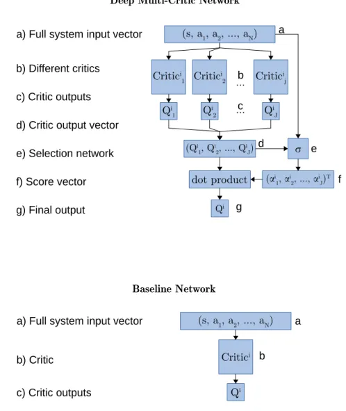
Fig. 1. Network architectures for the Baseline and Deep Multi-Critic Network.
networks with a varying number of features. The proposed Deep Multi-Critic Network architecture, illustrated inFig. 1, attempts to overcome both obstacles.
The architecture is defined as follows. First, we initialisej Crit-icsQi
j(s
,
a|
θ
ji) of different complexity for agenti∈ {
1,
2, . . . ,
N}
. Then, we feed the centralised observationO=
(s,
a1,
a2, . . . ,
aN) through each Critic and obtain a vector consisting of j Critic outputs:−
→
Qi
=
(Q1i(O|
θ
1i),
Q2i(O|
θ
2i), . . . ,
Qji(O|
θ
Ni)).
A selection networkfcalculates a score for each of the Critics
−
→
α
=
f(O
,
−
→
Qi
|
σ
)T=
(α
1, α
2, . . . , α
j)T,
which are used to produce the final output of the network: a weighted sum over the Critic outputs
Qi
=
−
→
Qi·
−
→
α
=
−
→
Qi·
f(O,
−
→
Qi|
σ
)T=
∑
jα
jQji(O|
θ
ji).
By combining the outputs of different Critics, each individual bias will be less prominent in the total output. Moreover, as no single Critic is responsible for the Q values alone, the responsibility is distributed among the Critics, so that a large change in one Critic will not have a great impact on the total output of the system.
The number of units in each hidden layer is defined as K
∑
i=1
dim(oi)
+
dim(ai),
i∈ {
1, . . . ,
N}
,
where dim(oi)
+
dim(ai) is the sum of the dimensions of agenti’s observation and action space. All hidden layer activation func-tions are ReLUs. The Critics have no activation function in the final layer, the selection network has a softmax activation function for producing scores that sum to 1.
3.3. Baseline network architecture
Deep Multi-Critic Network is compared to the Baseline net-work, which is the simplest Deep Neural Network with 2 fully connected hidden layers and ReLU activation functions. The main goal of Deep Multi-Critic Network is to achieve better generalisa-tion compared to Baseline. The number of trainable parameters in Baseline is 4418, while Deep Multi-Critic Network has 48 349. By having substantially more parameters, Deep Multi-Critic Net-work should in theory be prone to overfitting compared to the relatively simple Baseline network. The challenge is to achieve better generalisation performance with a more complex model.
The Baseline architecture was chosen by performing a search over a grid of parameters. For each combination of parameters, 10-fold cross-validation was used to find the best performing
Table 2
Parameters searched over for the baseline architecture.
Parameter name Values
L1 regularisation 0.1, 0.001, 0.0001
No. of hidden layers 1, 2, 3
Epochs trained 1, 2, 3, 4, 5
Learning rate 0.1, 0.01, 0.001, 0.0001
Table 3
Football tracking data overview.
Property Value
Tracking data capture rate 10 Hz
Number of sequences 7500
Average sequence length 176 steps
Minimum sequence length 50 steps
Maximum sequence length 1480 steps
Sequence length standard deviation 133 steps
Total steps in all sequences 1321.7 k
Number of features 46
Features per agent (incl. ball) 2
model. Data used for performing the search originated from a single player, leaving us with the data of 21 other players for testing. Each fold was trained with 80% of training data and was validated on the hold-out 20% data. This was done in order to find the optimal complexity of the network when enough data has been generated. Because we know the optimal complexity and parameters beforehand, we can see how the network performs when very little data is available. The score for a parameter combination was the mean absolute prediction error on hold-out data for each fold. The parameters searched over are presented in
Table 2.
3.4. Comparisons to COMA and MADDPG
In addition to comparing DMCN to Baseline, we also compare it to COMA and MADDPG critics. Moreover, we also present results for another configuration based on the DMCN approach, called DMCN 128/8. The architectural idea behind the network is the same as before, but now we are using subnetworks with widths
w
∈ {
8,
16, . . . ,
128}
, in order to investigate the prop-erties of a similar architecture with more complex subnetworks. Finally, observing results using a similar, but different architec-ture gives us more evidence either for or against the proposed solution’s effectiveness.4. Experimental results and discussions
4.1. Description of the dataset
The data used for conducting the experiments contains track-ing data from 7500 football gameplay sequences, collected at 10 Hz. The data consists of the (x
,
y) coordinates of the players and the ball recorded from to a top–down view of the football court. The gameplay sequences are of varying length and in total correspond to roughly corresponding 45 games worth of playing time. Each sequence starts with the attacking team possessing the ball and ends with them losing control of the ball — this has been done in order to reduce the amount of ‘dead time’ in the learning examples. The data has been prepared so that the attacking team always moves from left to right. The data is available here (LLC,2018).
For a more detailed overview of the data, please refer to
Table 3.
Training data for the Critics, which consist of input–output pairs, were generated from gameplay sequences as follows. Each gameplay sequence is in matrix formST×F, whereT is the length
Table 4
The training set sizes used.
% of data 0.0125 0.025 0.05 0.1 0.2 0.5 1
Nr. of samples 82 165 329 659 1318 3295 6589
Table 5
Proposed solution (DMCN) compared to Counterfactual Multi-Agent Policy Gra-dient (COMA) and Multi-Agent Deep Deterministic Policy GraGra-dient (MADDPG) critics. Values presented in the table are test losses, measured and averaged over 30 different runs.
DMCN COMA MADDPG DMCN 128/8 Data (%)
0.511 0.395 0.54 0.368 0.0125 0.379 0.236 0.414 0.213 0.025 0.177 0.111 0.23 0.073 0.05 0.0588 0.057 0.108 0.025 0.1 0.024 0.03 0.051 0.011 0.2 0.008 0.012 0.018 0.004 0.5 0.004 0.006 0.007 0.002 1.0
of the sequence andF is the number of features (46). FromST×F we create input–output pairs for agenti
(St,:
,
St+1,2i:2i+1),
t∈ {
1,
3, ...,
2⌊
T
2
⌋ +
1}
.
The training data was standardised to have 0 mean and a standard deviation of 1. Test data was standardised with the parameters used for training data.
4.2. Effects of Curse of Dimensionality
The main purpose of Deep Multi-Critic Network is to reduce the effects of Curse of Dimensionality when training Central Critics. However, there is more than enough data when gameplay sequences are turned to input–output pairs. In order to see the effects of Curse of Dimensionality, very small subsets of available data are used to train the Baseline and Deep Multi-Critic Network models. The small subsets are randomly sampled from training data repeatedly for various subset sizes. This is done to simulate the model’s learning performance in different stages of data avail-ability. Test data is also sampled randomly, without overlapping with training data. Both models get trained and tested on the same data in order to provide as fair of a comparison as possible. For each subset of training and testing data, both Baseline and Deep Multi-Critic Network model are instantiated, trained and tested 30 times. Training dataset sizes range from 0.125% to 1% of available data, with each successive dataset doubling in size (see Table 4). Both models are trained for 10 epochs and their performance on test data (20% of available data, sampled randomly) is calculated after each epoch. This allows us to see if and when the models stop generalising and start overfitting. After completing 30 runs, the metrics are averaged to produce an aggregated view of model performance.
4.3. Results
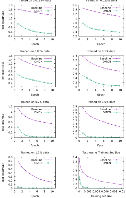
The experimental results show that Deep Multi-Critic Net-work’s test loss is significantly lower than Baseline’s on all tested training set sizes (Fig. 2). Although Deep Multi-Critic Network contains more than 10 times the trainable parameters in the Baseline model, the performance advantage for Deep Multi-Critic Network is preserved even when 0.05% of data is used for train-ing. Intuitively, such a complicated model will likely overfit. The gap between Baseline and Deep Multi-Critic Network perfor-mance becomes smaller as training progresses, allowing Baseline to catch up to Deep Multi-Critic Network. However, the no-ticeable gap between the models remains, even as more data becomes available.
Fig. 2. Baseline vs. Deep Multi-Critic Network (DMCN) performance on the test sets.
The results suggest that Deep Multi-Critic Network uses avail-able data more efficiently than the Baseline model. In each train-ing data setttrain-ing, the loss gap between Baseline and Deep Multi-Critic Network after the first epoch is between 0.7 and 0.8. The gap between the losses of Baseline and Deep Multi-Critic Network shrinks from 0.8 down to 0.2 as the networks are trained with more data.
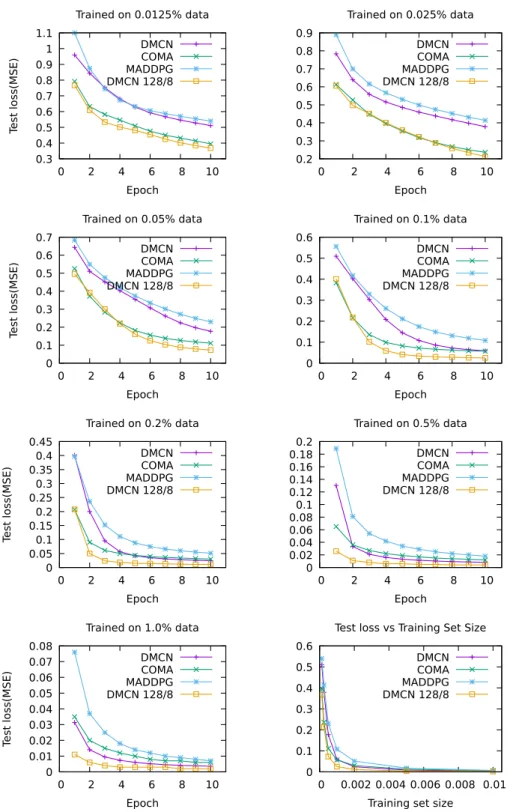
Comparing the proposed approach (DMCN) to the critics of Multi-Agent Deep Deterministic Policy Gradients (MADDPG) and Counterfactual Multi-Agent Policy Gradients (COMA), COMA comes ahead in the three smallest data settings, with DMCN
maintaining an advantage over MADDPG (Fig. 3. Starting from the fourth smallest data setting (0.1%), the performance gap between DMCN and COMA closes (0.059 vs. 0.057, respectively), with DMCN coming ahead in other experiments (Table 5). However, DMCN 128/8 can achieve better performance compared to COMA in all available data settings.
4.4. Discussion
In order to understand how Deep Multi-Critic Network achieves good performance, we investigate the change in Critic
Fig. 3. Deep Multi-Critic Network (DMCN) compared to Counterfactual Multi-Agent Policy Gradient (COMA) and Multi-Agent Deep Deterministic Policy Gradient (MADDPG) critics.
scores. As the output of Deep Multi-Critic Network is a weighted sum of Critics, with the weights given by the Selection network, observing the scores gives us insight into how Critic contribu-tions change during training and with increasing the amount of training data.
To visualise the scores, Deep Multi-Critic Network was trained 30 times on sampled data for each dataset size for 10 epochs. The scores were produced by evaluating the model on test data (20%) after each training epoch and collecting the Selection network’s outputs. After collection, the scores were averaged to produce the mean score for each Critic during each training epoch.
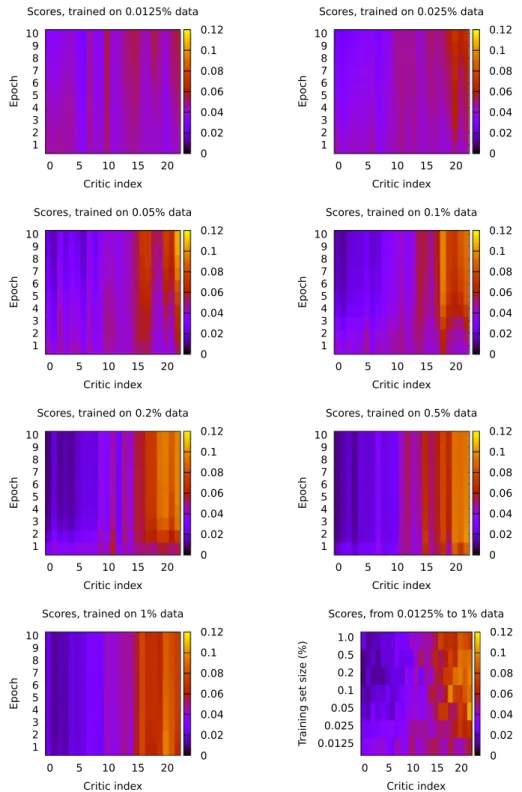
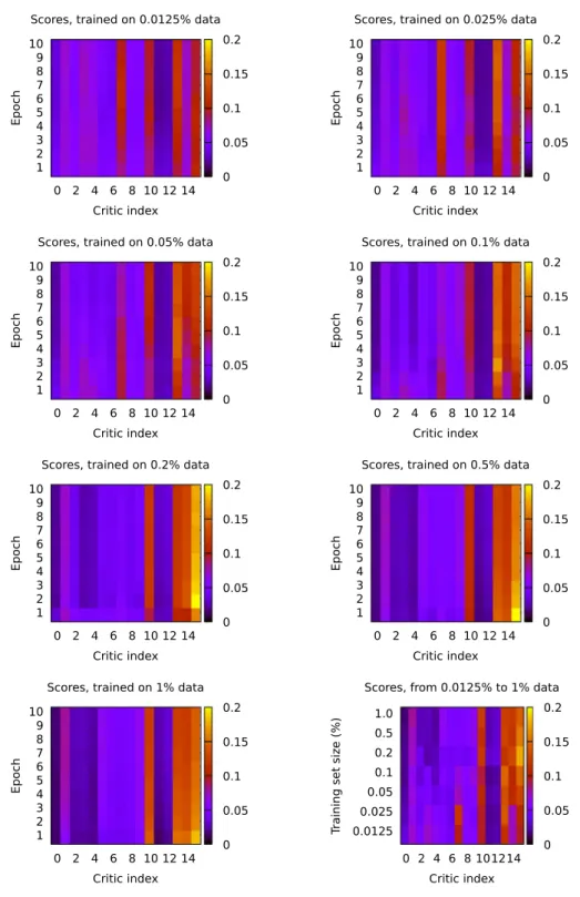
Average scores indicate that once more training data becomes available, more complex Critics are given a higher score (Fig. 4). With the lowest data setting, scores are distributed rather uni-formly, even after the last training epoch, which shows that no single Critic is a distinct contributor to the output. In higher data settings, the score distribution moves towards the right in the direction of more complex Critics, indicating the higher contri-bution of larger subnetworks to the overall output. Intuitively, as the more complex critics are exposed to more data, they get increasingly accurate compared to the smaller critics. The smaller critics are limited by their capacity, enabling more complex critics
Fig. 4. Average scores for DMCN Critics during training.
to contribute more to the overall output as more data becomes available for the multi-critic network.
Compared to the Baseline Network, the proposed Deep Multi-Critic Network with its many Multi-Critics achieved equivalent per-formance earlier during training and achieved an overall lower loss, suggesting the ability to learn more from the same amount of data. Even though Deep Multi-Critic Network contains more than 10 times the parameters in the Baseline Network, over-fitting did not occur and the generalisation performance was better than the baseline model in all experiments. This effect can be attributed to the distribution of responsibility: no single subnetwork is responsible for the final output alone, but selected subnetworks can learn to contribute more than others. Deep
Multi-Critic Network’s performance is comparable with critics from other approaches (COMA and MADDPG). Although DMCN and DMCN 128/8 have a more complex architecture with more neurons, they manage to achieve competitive performance com-pared to COMA and MADDPG without overfitting to the small amounts of training data. Interestingly, DMCN 128/8, with a more complicated architecture (approximately 152k parameters), of-fers better performance in low-data settings compared to the original DMCN, possibly indicating an enhanced ability to learn from the same amount of experience. Looking at the critic scores
inFig. 5, we observe a similar pattern of critic scores inFig. 4. In
both cases, higher complexity critics contribute more to the final output of the network, with some critics of moderate complexity
Fig. 5. Average scores for DMCN 128/8 Critics during training.
having a noticeable score as well. Again, we hypothesise that the performance gains are achieved by distributing responsibility among critics and leveraging the possibility of combining the outputs of models, each of various capacity.
5. Conclusions and future work
Overcoming the issue of Curse of Dimensionality associated with multi-agent reinforcement learning is crucial for the suc-cess of many applications that require policy learning in multi-agent settings. Paying attention to only a subset of features is an avenue that researchers have recently focused on. However, implementing such feature selection, in real-world environments
is a challenging concept to implement, because of the com-binatorial explosion of feature combinations to select and the inability of Deep Neural Networks to work with inputs of varying size. To overcome this issue, this paper presents an ensemble of critic networks is trained, which performs a context depen-dent summation of the results. The proposed Deep Multi-Critic Network, which is proposed as a method for reducing the ef-fects of Curse of Dimensionality, was shown to have an ability to learn faster from fewer samples, in a multi-agent learning environment. The proposed methodology to simplify the learning process in a Multi-agent scenario is a step towards enhancing the effectiveness of data driven policy learning.
Future work is necessary to investigate efficient ways for finding the optimal architectures of the Critics — their number, width, depth and other parameters, as we believe this to be very problem-dependent. Furthermore, it is necessary to determine how the addition of Deep Multi-Critic Network will affect the convergence of the Critic in Actor–Critic methods to further val-idate the findings. Finally, we intend to investigate how strongly the initial weights of Deep Multi-Critic Network determine which Critics receive higher scores during training.
Declaration of competing interest
The authors declare that they have no known competing finan-cial interests or personal relationships that could have appeared to influence the work reported in this paper.
Acknowledgement
This work was funded by the Engineering and Physical Sci-ences Research Council in the United Kingdom, under grant number EP/T000783/1: MIMIC: Multimodal Imitation Learning in Multi-Agent Environments
References
Buşoniu, L., Babuška, R., & De Schutter, B. (2010). Multi-agent reinforcement learning: An overview. (pp. 183–221). http://dx.doi.org/10.1007/978-3-642-14435-6_7, URLhttp://link.springer.com/10.1007/978-3-642-14435-6_7. Choi, J., Lee, B.-J., & Zhang, B.-T. (2017). Multi-focus attention network for
efficient deep reinforcement learning. InWorkshops at the thirty-first AAAI conference on artificial intelligence.
Finn, C., Levine, S., & Abbeel, P. (2016). Guided cost learning: Deep inverse op-timal control via policy optimization. InInternational conference on machine learning(pp. 49–58).
Foerster, J. N., Farquhar, G., Afouras, T., Nardelli, N., & Whiteson, S. (2018). Counterfactual multi-agent policy gradients. InThirty-Second AAAI conference on artificial intelligence.
Goertzel, B. (2014). Artificial general intelligence: concept, state of the art, and future prospects.Journal of Artificial General Intelligence,5(1), 1–48. Iqbal, S., & Sha, F. (2018). Actor-attention-critic for multi-agent reinforcement
learning. arXiv preprintarXiv:1810.02912.
Konda, V. R., & Tsitsiklis, J. N. (2000). Actor-critic algorithms. InAdvances in neural information processing systems(pp. 1008–1014).
Laurent, G. J., Matignon, L., & Fort-Piat, L. (2011). The world of independent learners is not Markovian. International Journal of Knowledge-Based and Intelligent Engineering Systems,15(1), 55–64.
LLC, S. (2018). Data science | STATS. URL https://statstesting.wpengine.com/data-science/.
Lowe, R., Wu, Y., Tamar, A., Harb, J., Abbeel, O. P., & Mordatch, I. (2017). Multi-agent actor-critic for mixed cooperative-competitive environments. In Advances in neural information processing systems(pp. 6379–6390). Mnih, V., Kavukcuoglu, K., Silver, D., Graves, A., Antonoglou, I., Wierstra, D., &
Riedmiller, M. (2013). Playing atari with deep reinforcement learning. InNIPS deep learning workshop, Harrah’s Sand Harbor, Lake Tahoe, USA.
Mnih, V., Kavukcuoglu, K., Silver, D., Rusu, A. A., Veness, J., Bellemare, M. G., et al. (2015). Human-level control through deep reinforcement learning. Nature,518, 529, URLhttps://doi.org/10.1038/nature14236 http://10.0.4.14/ nature14236 https://www.nature.com/articles/nature14236#supplementary-information.
Schulman, J., Levine, S., Abbeel, P., Jordan, M., & Moritz, P. (2015). Trust region policy optimization. In International conference on machine learning (pp. 1889–1897).
Silver, D., Hubert, T., Schrittwieser, J., Antonoglou, I., Lai, M., Guez, A., et al. (2018). A general reinforcement learning algorithm that masters chess, shogi, and Go through self-play.Science,362(6419), 1140–1144.
Silver, D., Lever, G., Heess, N., Degris, T., Wierstra, D., & Riedmiller, M. (2014). Deterministic policy gradient algorithms.
Silver, D., Schrittwieser, J., Simonyan, K., Antonoglou, I., Huang, A., Guez, A., et al. (2017). Mastering the game of Go without human knowledge. Na-ture, 550(7676), 354–359.http://dx.doi.org/10.1038/nature24270, URLhttp: //www.nature.com/doifinder/10.1038/nature24270.
Sorokin, I., Seleznev, A., Pavlov, M., Fedorov, A., & Ignateva, A. (2015). Deep attention recurrent Q-network. arXiv preprintarXiv:1512.01693.
Sutton, R. S., & Barto, A. G. (2018).Reinforcement learning: An introduction. MIT press.
Watkins, C. J. C. H., & Dayan, P. (1992). Q-learning. Machine Learning, 8(3), 279–292.http://dx.doi.org/10.1007/BF00992698.