Magn Reson Med. 2019;81:1979–1992. wileyonlinelibrary.com/journal/mrm
|
1979F U L L PA P E R
Model‐based reconstruction framework for correction of signal
pile‐up and geometric distortions in prostate diffusion MRI
Muhammad Usman
1|
Lebina Kakkar
2|
Alex Kirkham
3|
Simon Arridge
1|
David Atkinson
21Centre for Medical Image Computing, Department of Computer Science, University College London, London, United Kingdom 2Centre for Medical Imaging, Division of Medicine, University College London, London, United Kingdom
3Department of Radiology, University College Hospital, London, United Kingdom
© 2018 The Authors Magnetic Resonance in Medicine published by Wiley Periodicals, Inc. on behalf of International Society for Magnetic Resonance in Medicine
This is an open access article under the terms of the Creative Commons Attribution License, which permits use, distribution and reproduction in any medium, provided the original work is properly cited.
Correspondence
Muhammad Usman, Centre for Medical Image Computing, Department of Computer Science, University College London, Gower Street, London, WC1E 6BT, United Kingdom.
Email: [email protected]
Funding Information
Cancer Research UK/EPSRC (grant A21099) and the NIHR Biomedical Research Unit at UCH
Purpose: Prostate diffusion‐weighted MRI scans can suffer from geometric distor-tions, signal pileup, and signal dropout attributed to differences in tissue susceptibil-ity values at the interface between the prostate and rectal air. The aim of this work is to present and validate a novel model based reconstruction method that can correct for these distortions.
Methods: In regions of severe signal pileup, standard techniques for distortion cor-rection have difficulty recovering the underlying true signal. Furthermore, because of drifts and inaccuracies in the determination of center frequency, echo planar imag-ing (EPI) scans can be shifted in the phase‐encodimag-ing direction. In this work, usimag-ing a B0 field map and a set of EPI data acquired with blip‐up and blip‐down phase
encod-ing gradients, we model the distortion correction problem linkencod-ing the distortion‐free image to the acquired raw corrupted k‐space data and solve it in a manner analogous to the sensitivity encoding method. Both a quantitative and qualitative assessment of the proposed method is performed in vivo in 10 patients.
Results: Without distortion correction, mean Dice similarity scores between a refer-ence T2W and the uncorrected EPI images were 0.64 and 0.60 for b‐values of 0 and 500 s/mm2, respectively. Compared to the Topup (distortion correction method com-monly used for neuro imaging), the proposed method achieved Dice scores (0.87 and 0.85 versus 0.82 and 0.80) and better qualitative results in patients where signal pi-leup was present because of high rectal gas residue.
Conclusion: Model‐based reconstruction can be used for distortion correction in prostate diffusion MRI.
K E Y W O R D S
1
|
INTRODUCTION
Prostate cancer is the most commonly diagnosed cancer in males and the second cause of cancer‐related deaths in men.1
Early detection of prostate cancer can help in better manage-ment and treatmanage-ment of disease when the cancer is still local-ized. Multiparametric prostate magnetic resonance imaging (mpMRI) is now becoming a common tool for early detection and staging of prostate cancer. Typically, mpMRI is done as a combination of T2‐weighted (T2W), diffusion‐weighted MRI (DWI), and dynamic contrast‐enhanced MRI (DCE) scans, which determine the likelihood of clinically significant cancer at a particular location within prostate.2,3 DWI is the
main sequence for cancer detection in the peripheral zone of the prostate,4 where 75% of tumors usually occur.5 Prostate
cancers normally show abnormal diffusion restrictions and high signal in DWI images.
In DWI, single‐shot echo planar imaging (SS‐EPI) has been the preferred k‐space read out technique because of its fast speed and robustness against motion artefacts. However, SS‐EPI has a disadvantage of low bandwidth along the phase‐ encoding direction, making it sensitive to inhomogeneities in the magnetic field. In MRI, spatial encoding is achieved by using magnetic field gradients, and the measured signal rep-resents the Fourier transform of the object. In the presence of magnetic field inhomogeneities, an additional off‐resonance field (called B0 field) will add an additional component to the
linear magnetic field gradient so that the position‐frequency relationship is changed. This results in signal stretching in areas within the image where the gradient of B0 field has the
same polarity as the phase‐encoding gradient. Conversely, signal compression or pileup occurs in regions where the B0 field gradient direction is opposite to that of the phase‐
encoding gradient. This results in multiple pixels along the phase‐encoding direction being merged into a single pixel. The main source of B0 field inhomogeneities is the
suscep-tibility differences that arise at the interface between tissues of different susceptibilities. Larger local susceptibility differ-ences will create a stronger off‐resonance field that will result in more‐severe signal pileup or stretching within the image. For DWI prostate images, susceptibility differences result in severe distortions and poor depiction of zonal anatomy.6 This
can result in nondiagnostic images, errors in image interpre-tation, or a requirement for biopsy. Additionally, DWI images from prostate cancer patients with metallic hip prostheses7
may also suffer from susceptibility‐induced distortions across the whole prostate region. In addition to susceptibility‐ induced distortions, a translational shift may occur along the phase‐encoding direction8 in the reconstructed EPI images
attributed to drifts in center frequency of the magnet. Several methods have been proposed to address the B0
distortion problem in EPI images. Some of these techniques correct distortions directly in the image space using a B0 field
calculated from a separate dual‐echo gradient echo scan.9-12
Having an accurate B0 field, these methods can generally
cor-rect for signal‐stretching artefacts in the images. However, using EPI data acquired with only 1 phase‐encoding direction may not provide sufficient information to correct for signal pile‐up artefacts. To address this issue, image‐registration– based reverse‐phase–encoded gradient methods have been proposed for brain functional MRI that acquire the same slice twice with opposite phase‐encoding gradient directions, re-sulting in 2 data sets, blip‐up and blip‐down.8,13 Using the
assumption that the signal pile‐up effects with blip‐up data set will correspond to the signal‐stretching effects in the same region with blip‐down data set and vice versa, these methods attempt to find the B0 field as a symmetrical displacement
field by using image registration that will result in identical corrected images in the 2 phase‐encoding gradient direc-tions. However, instead of solving the full inverse problem constrained to the acquired raw k‐space data, these methods perform image‐based optimization. This may result in an erroneous calculation of the B0 field attributed to the lack
of a unique solution between the corresponding locations in the blip‐up and blip‐down images (especially in regions with severe signal pileup),14 leading to artifacts or blurring
in the final images. Furthermore, in image‐based methods, the registration becomes more difficult when the image sig-nal‐to‐noise ratio (SNR) is poor15,16 and registration errors
may lead to failure in distortion correction. By defining a forward model linking the distortion free image to the ac-quired corrupted raw k‐space data, an exact solution of the full inverse problem may be achieved by using the forward and conjugate transpose operators with a conjugate gradient scheme.17 Distortions attributed to B
0 field inhomogeneities
may be corrected directly during the reconstruction process using this full inverse problem solution, although a previous estimation of the B0 field is needed. The complex
averag-ing used in the reconstruction avoids the bias from noise that can occur when magnitude images are combined.18-21 This is
likely to be especially beneficial for high b‐value DWI im-ages with low SNR.18,20,21
In this work, we propose a model‐based reconstruction framework to solve the full inverse problem of prostate DWI distortion correction. By using the EPI raw k‐space data from acquisitions with blip‐up and blip‐down phase‐encoding gra-dients, we model the distortion correction problem linking the corrupted k‐space data to the corrected image and solve it in a manner analogous to sensitivity encoding (SENSE),22 using
the conjugate gradient (CG) iterative method. To solve the issue of translational shifts attributed to the uncertainties in center frequency, we include the centre frequency offset cor-rection as an initial unknown in our framework. In addition, a phase correction is also incorporated into our framework to avoid any phase cancellation issues that may arise because of small motion of the tissue within the diffusion‐encoding
gradients. Results using the proposed method are compared in 10 patients against a neuroimaging distortion correction method based on reverse‐phase–encoding gradient, known as Topup.8
2
|
METHODS
2.1
|
Acquisition
The proposed framework acquires 2 EPI data sets (blip‐up and blip‐down) with opposite phase‐encoding gradient direc-tions. A B0 scan is acquired as a separate dual‐echo gradient
echo scan for estimation of the B0 field.
2.2
|
Reconstruction
With B0 field inhomogeneities, the corrupted k‐space Yj
cor-responding to jth coil (j = 1, 2,…,J; J being total number of
coils) can be related to the undistorted image x by the follow-ing model (Equation 1):
where m, n are image coordinate indices, M, N are image dimensions, k, l are k‐space coordinate indices, t(k, l) is the sample time for location (k, l) in k‐space, ΔB0 is the B0 field
in Hz that is estimated from a separate dual echo gradient echo scan, Cj is the jth coil sensitivity, and j = 1, 2,..,J
In the presence of a center frequency offset (∆f0), the
model in Equation 1 is modified as Equation 2:
In the above expression, the center frequency offset ∆f0
is assumed to be a constant in space. For a given ∆f0,
trans-lational shifts in image space are equal and opposite for op-posite phase‐encoding gradient directions (e.g., positive shift for blip‐up and negative for blip‐down scans or vice versa).
2.3
|
Proposed Framework
The proposed reconstruction framework has the following 3 steps.
2.3.1
|
Step 1. Estimation of center
frequency offset (∆
f0
)
Let Yj1 and Yj2 be the k‐space for blip‐up and blip‐down EPI
scans for jth coil, respectively. Mathematically, we can write
(Equation 3):
where t1 and t2 are the acquisition times of the k‐space
sam-ples for blip‐up and blip‐down scans, respectively. Equation 3 can be summarized as Equation 4:
where Ej1 and Ej2 are the encoding operators for blip‐up and
blip‐down scans, respectively. The preliminary model‐based conjugate phase reconstructions (xcp1 and xcp2) from
multi-coil data are calculated as a multimulti-coil combination, where the jth coil contribution is obtained by performing adjoint of en-coding operators Ej1 and Ej2 onto the corresponding k‐space Yj1 and Yj2, respectively.
Mathematically, xcp1 and xcp2 are expressed as Equation 5:
where(⋅)H is the Hermitian operator.
The optimal center frequency offset ∆f0,opt is estimated as a parameter that maximizes the mutual information (MI) similarity measure23 between preliminary model‐based
conjugate phase reconstructions of the blip‐up and blip‐ down EPI data (xcp1 and xcp2) acquired with a b‐value of
0 s/mm2 by solving the following unconstrained problem
(Equation 6):
The B0 field is corrected by updating it with estimated
optimal center frequency offset ∆f0,opt. The definition of Mutual Information function used in our method is described in Appendix I.
2.3.2
|
Step 2. Phase correction
For diffusion‐weighted data (b‐value > 0 s/mm2), the phase
of the blip‐up and blip‐down data in the image space might be different because of small physiological motion that may occur during the diffusion sensitization gradients. If data (1) Yj(k,l) = N−1 ∑ n=0 M−1 ∑ m=0 Cj(m,n)x(m,n)e−i2𝜋(mkM+ nl N)e−i2𝜋(𝚫B0(m,n).t(k,l)) (2) Yj(k,l) = N−1 ∑ n=0 M−1 ∑ m=0 Cj(m,n)x(m,n)e−i2𝜋( mk M+ nl N)e−i2𝜋((𝚫B0(m,n)+Δf0).t(k,l)) Yj1(k,l) = N−1 ∑ n=0 M−1 ∑ m=0 Cj(m,n)x(m,n)e−i2𝜋(mkM+ nl N)e−i2𝜋((𝚫B0(m,n)+Δf0).t1(k,l)) (3) Yj2(k,l) = N−1 ∑ n=0 M∑−1 m=0 Cj(m,n)x(m,n)e−i2𝜋 ( mk M+ nl N ) e−i2𝜋((𝚫B 0(m,n)+Δf0).t2(k,l)) Yj1=Ej1x (4) Yj2=Ej2x xcp1= J ∑ j=1 (Ej1)HYj1 (5) xcp2= J ∑ j=1 (Ej2)HYj2 (6) Δf0,opt=argΔf 0max (MI ( xcp1,xcp2))
are combined from the 2 phase‐encoding directions without phase correction, this may result in phase cancellation lead-ing to signal dropout in the final reconstructed image. To cater for this issue, we propose to calculate a phase correction ∆Ф obtained by taking the Hermitian inner product between the preliminary model‐based conjugate phase reconstructions (xcp1 and xcp2) of blip‐up and blip‐down EPI data using
cor-rected B0 field (Equation 7):
where <.> indicates the inner product, (.)* denotes the com-plex conjugate, and m, n are image coordinate indices. In the above expression, the phase correction ΔФ varies in space because of the spatial variance of phases in xcp1 and xcp2. The
raw k‐space data are corrected in phase by applying the phase correction ΔФ in the image space as follows.
With k‐space Yj2 selected as a reference, phase correction
was applied to Yj1 by (1) first applying the inverse Fourier
transform (IFT) to it, (2) multiplying by an exponential term containing the phase correction ΔФ to get the corrected image ỹj1, and (3) transforming back to k‐space by the Fourier transform (FT) to get a final phase‐corrected k‐space Ỹj
1.
Mathematically (Equation 8),
2.3.3
|
Step 3. Model‐based reconstruction
The phase‐corrected multicoil k‐space data Ỹ
1and Ỹ2 and
the encoding operators E1 and E2 for blip‐up and blip‐down
scans can be expressed mathematically by stacking data and encoding operators from all J coils (Equation 9):
Using the center frequency offset corrected ΔB0 obtained
from step 1, for each b‐value and diffusion direction, the phase‐corrected EPI data Ỹ
1 and Ỹ2 can be combined into a
single formulation by setting Ỹ=[Ỹ
1Ỹ2]T and E = [E1 E2]T
in Equation 2. Model‐based reconstruction is done (Figure 1a) from combined k‐space data Ỹ in a manner anal-ogous to an iterative SENSE reconstruction22 based on the
conjugate gradient method by solving the following minimi-zation problem (Equation 10):
The above minimization problem is strictly convex be-cause the encoding operator E is a linear function in x. Large negative local B0 field gradients in the phase‐encoding
di-rection can make the encoding operator E1 or E2 singular or
badly ill‐conditioned.12 The convergence of the CG iterations
is achieved when the normalized residual r=||EHEx−EHỸ||2 ||EHỸ||
2
(||⋅||2 denotes the l2 norm) in the current iteration becomes
smaller than ϵ (ϵ being a small number) giving the final dis-tortion corrected output image ẋ.
Figure 1b and Figure 1c shows visual illustrations for details of implementation of forward and adjoint encoding operators Ei and EHi, respectively; i = 1 and i = 2 refer to blip‐
up and blip‐down scans, respectively. The forward encoding operator Ei involves multiplication of input image x by
in-dividual coil sensitivities Cj that is followed by a modified Fourier transform operator G that maps the product of image and coil sensitivity from image to Fourier space, taking into account the susceptibility effects determined by B0 field and
phase‐encoding direction dependent k‐space sampling times ti. The adjoint encoding operator EHi involves transforming
each individual coil k‐space data to image space by adjoint of modified Fourier transform operator (GH) followed by multiplication by the corresponding complex conjugated coil sensitivity (Cj)* and the final summation over all the coils.
2.4
|
Experiments
Ten male patients (median weight, 84 [range, 68–98] kg and age 68 [57–79] years old) were recruited from the clinical prostate imaging pathway and were consented for additional image acquisitions. No antispasmodic agent was adminis-tered. Patients were placed feet first into the scanner and im-aging was carried out during free breathing for all patients. The study was approved by the ethics committee, and written signed consent was obtained from all patients for the research scans.
Scanning was performed on a 3T scanner (Achieva; Philips Healthcare, Best, The Netherlands) equipped with 16 ante-rior + 16 posteante-rior channel receive coil array. Single‐shot EPI data in both blip‐up and blip‐down phase‐encoding directions were acquired. The EPI scans had the following parameters: resolution = 2 × 2 × 4 mm3, field of view (FOV) = 180 to
220 × 180 to 220 × 55 to 90 mm3, partial Fourier acquisition
with half scan factor of 0.75, TE/TR = 80 msec/2500 msec, phase‐encoding direction = anterior‐posterior (AP) axis with fat shift in the direction “P” for blip‐up and direction “A” for blip‐down scans, b‐values = 0 and 500 s/mm2, number of
isotropic diffusion directions = 3, number of averages = 3, phase‐encode bandwidth per pixel = 10.4 to 11.2 Hz/pixel, and scan time = 30 sec. For calculation of the B0 field, a
separate 3D dual‐echo gradient echo scan was acquired with the following parameters: resolution = 2 × 2 × 2 mm3, FOV
(7) Δ𝚽(m,n)=angle<xcp1(m,n),x∗ cp2(m,n)> Step a: yj1←IFT←Yj1 Step b:ỹj1=yj1exp (−iΔ𝚽) (8) Step c:ỹj1→FT→Ỹj1 ̃ Y1=[Ỹ1 1 ̃ Y21⋅ ⋅ ⋅ ⋅ỸJ 1] T ⋅ ⋅ ⋅and⋅ ⋅Ỹ2=[Y 1 2Y 2 2⋅ ⋅ ⋅ ⋅Y J 2] T (9) E1=[E11E21⋅ ⋅ ⋅ ⋅EJ1]T ⋅ ⋅ ⋅ ⋅and⋅ ⋅ ⋅ ⋅E2=[E 1 2E 2 2⋅ ⋅ ⋅ ⋅E J 2] T (10) minx||E H Ex−EHỸ||22
= 200 to 250 × 200 to 250 × 70 to 120 mm3, flip angle = 6°,
right to left phase‐encoding direction, SENSE acceleration factor = 1, TE difference (ΔTE) = 2.3 msec, TE1/TE2/TR = 4.6/6.9/8.7 msec, and scan time = 1 minute. For reference, axial T2W images were acquired using a turbo spin echo scan with the following parameters: resolution = 2 × 2 × 4 mm3,
FOV = 180 to 220 × 180 to 220 × 55 to 90 mm3, SENSE
acceleration factor = 2, TE/TR = 100/4700 msec, and scan time = 40 sec. Volume shimming was performed to cover the whole prostate and surrounding areas.
2.5
|
Data Postprocessing
To save the raw data together with the relevant information needed for the reconstruction framework, a software patch was implemented using ReconFrame software (Gyrotools Zurich, Zurich, Switzerland). EPI phase correction was performed using the ReconFrame tool to correct for ghosts originating from alternating offsets of phase encode lines in k‐space. Subsequent postprocessing was implemented in MATLAB (The MathWorks, Inc., Natick, MA).
The B0 field was calculated using the quantitative sus-ceptibility mapping toolbox24 that estimates the field by a
weighted least squares fit of temporally unwrapped phases in each voxel over echo time. A robust spline‐based smoothing25
was applied to the B0 field in image domain to smooth out noisy components. The 3D B0 field and T2W images were
re-sampled to match the EPI scan resolution and the associated FOV. The iterative optimization in Equation 6 to estimate the optimal center frequency offset Δf0,opt was carried out using the fminsearch function in MATLAB that uses the Nelder‐ Mead simplex algorithm.26 The number of iterations in the
algorithm was set to 10, and the optimal frequency offset Δf0,opt was set to the value of Δf0 found in the last iteration.
This was followed by phase correction (Equations 7 and 8) and model‐based reconstruction in Equation 10. The threshold ∊ for convergence of CG iterations in Equation 10
was set to 0.0025 in all our experiments. The model‐based corrected reconstruction was compared against uncorrected blip‐up and blip‐down reconstructions and the neuroimaging distortion correction Topup method.
2.6
|
Image Analysis
For quantitative evaluation, reconstructed images were con-verted to DICOM format and exported to Horos software,27
which is an open‐source medical image viewer. A region of interest (ROI) was manually drawn around the boundary of whole prostate in each T2W image and each reconstructed image by a radiologist with 12 years’ experience in reporting prostate MRI. Dice similarity coefficient scores28 were
com-puted from the ROI overlap of each reconstruction and the reference T2W image. For qualitative assessment, the images reconstructed with different methods were put in a random order and blinded to method to avoid subjective assessment. The radiologist scored each image in terms of resolution, dis-tortion, demarcation, and zonal anatomy.29 The “resolution”
was defined as the ability to recognize detailed anatomical structures within the prostate, and it was assessed on a 5‐ point scale (1 = poor; 2 = below average; 3 = average; 4 = above average; and 5 = excellent). The “distortion” was defined as the presence of artifacts, including signal pile‐up, signal dropout, warping, ghosting, and blurring. It was as-sessed on a 5‐point scale (1 = severe influence; 2 = signifi-cant influence; 3 = moderate influence; 4 = low influence; and 5 = no influence). The “demarcation” was defined as the ability to depict the prostatic capsule in a continuous fashion around the prostate. It was assessed on a 5‐point scale (1 = poor; 2 = below average; 3 = average; 4 = above average; and 5 = excellent). “Zonal anatomy” was defined as the abil-ity to distinguish the transitional zone of the prostate from the peripheral zone and was assessed on a 5‐point scale (1 = poor; 2 = below average; 3 = average; 4 = above average; and 5 = excellent).
FIGURE 1 Implementation of iterative model‐based reconstruction (step 3 of proposed framework) using data from both blip‐up and blip‐ down EPI scans. (a) Given the input k‐space data Ỹ
=[Ỹ1Ỹ2]
T that have been phase corrected in step 2, in each iteration of the conjugate gradient
(CG) algorithm, we iterate back and forth between the k‐space and image x by encoding operator E = [E1E2]T and its adjoint EH that include the center frequency offset corrected B0 field. The convergence is achieved when the residual r=EHEx−EHỸ2
EHỸ
2 in the current iteration becomes smaller
than ϵ (ϵ being a small number) giving the final distortion corrected output image ẋ. (b) Details of the forward encoding operator Ei that takes the input single image x to the multicoil output k‐space Yi for phase‐encoding direction i, i = 1 corresponds to the blip‐up and i = 2 corresponds to the blip‐down scans, respectively. The image x is first multiplied by the coil sensitivity Cj (j = 1, 2,..,J). This is followed by a modified Fourier
transform operator G that maps the product of image and coil sensitivity from image to Fourier space, taking into account the susceptibility effects determined by B0 field and k‐space sampling times ti, resulting in k‐space data Yji (j = 1, 2,..,J). (c) Details of the adjoint encoding operator EH
i
that takes the multicoil k‐space data Yji (j = 1, 2,..,J) to single image x for phase‐encoding direction i, i = 1 corresponds to the blip‐up and i = 2
corresponds to the blip‐down scans, respectively. Each individual coil k‐space data Yji is transformed to image space by the adjoint of a modified
Fourier transform operator (GH). The resulting images are individually multiplied by complex conjugated coil sensitivities (Cj i)
∗ (j = 1, 2,..,J) and
2.7
|
Phase correction procedures
The phase of DWI data (b‐value, >0 s/mm2) can change
dynamically because of small physiological motion occur-ring duoccur-ring the diffusion sensitization gradients. To evalu-ate the performance of the phase correction procedure used in our proposed framework, a mid‐prostate single slice was acquired for b‐value of 500 s/mm2 on 2 patients
for 40 dynamics with blip‐up phase‐encoding gradient. Model‐based reconstruction was done with and without phase correction for each pair of dynamics (dynamic 1 and dynamic 2, dynamic 1 and dynamic 3,….) in each diffu-sion direction with dynamic 1 selected as a reference. The goal is to check whether the proposed phase correction can work in cases where the dynamics have significantly different phases from one another in the conjugate phase reconstructions.
3
|
RESULTS
3.1
|
Estimation of center frequency offset
(∆f
0)
For all patients, the values of optimal center frequency off-set (in Hz) for a mid‐prostate slice are shown in Figure 2a, together with a convergence plot of objective function (nega-tive of mutual information function) as a function of iteration number in Figure 2b. The curve in Figure 2b shows that the objective function minimum (or equivalently mutual infor-mation function maximum) was achieved in 5 to 6 iterations. Mean frequency offset across all patients was 47.15 Hz with a standard deviation of 5.2 Hz.
3.2
|
Model‐based reconstruction
In Figure 3, for patient 1, the reference T2W image, the B0
field, uncorrected blip‐up and blip‐down reconstructions, correction using blip‐up data only and blip‐down data only, and proposed model‐based reconstructions are shown for b‐ values of 0 and 500 s/mm2, respectively. Because of
suscep-tibility differences at the interface between different tissues in the prostate region, the variation in B0 was around 120 Hz
that corresponds to a shift of 7 to 8 pixels at a bandwidth/ pixel of ~15.80 Hz in phase‐encoding direction. This resulted in pileup in regions where the B0 field gradient magnitude
was high and its direction was opposite to that of phase‐ encoding gradient (see regions pointed out by red arrows in Figure 3). The reconstruction results for patient 2 are shown in Figure 4. The proposed method corrected for signal pile‐ up artefacts that cannot be corrected using data from only 1 phase‐encoding gradient direction. For a mid‐prostate axial
slice in a selective group of 3 patients (patient 4, patient 6, and patient 9), the proposed and Topup reconstructions for b‐values of 0 and 500 s/mm2 are shown in Figures 5 and 6,
respectively. The complete set of results for patient 3 to patient 10 for b‐value of 0 and 500 s/mm2 can be seen in
Supporting Information Figures S1 and S2, respectively. Supporting Information Figure S3 shows an example plot of normalized residual error r as a function of CG iteration
num-ber. From our empirical observation, convergence of the CG method was achieved in 10 to 15 iterations.
Box plots showing the Dice scores for different recon-struction methods are shown in Figure 7. Mean Dice sim-ilarity scores were 0.60 (b‐value of 0) and 0.58 (b‐value of 500 s/mm2) for uncorrected blip‐up reconstructions and
0.68 (b‐value of 0) and 0.62 (b‐value of 500 s/mm2) for
un-corrected blip‐down reconstructions. The proposed method achieved mean Dice similarity scores of 0.87 and 0.85 for b‐value of 0 and 500 s/mm2, respectively, and scored
higher than the corresponding Dice similarity scores of the Topup method (0.82 and 0.80 for b‐value of 0 and 500 s/ mm2, respectively). Qualitative scores (distortion,
resolu-tion, demarcaresolu-tion, and zonal anatomy) for all 4 methods
FIGURE 2 In vivo results. (a) Estimated center frequency offset ∆f0 (measured in Hz) in mid‐prostate slice as a function of patient number. (b) Convergence of mutual information‐based optimization as a function of iteration number
corresponding to b‐value of 0 s/mm2 and b‐value of 500 s/
mm2 are given in Tables 1 and 2, respectively. Mean
per-centage of improvement in qualitative scores using the pro-posed method compared to other reconstructions is shown in Supporting Information Figure S4. The proposed method performed better, on average, than all other reconstructions for each qualitative measure.
3.3
|
Phase correction
Figure 8 shows the usefulness of phase correction used in the proposed method for patient 11 and patient 1 for data combined from a pair of dynamics acquired with diffusion weighting (b‐value of 500 s/mm2). Here, results are shown for
a pair of dynamics (dynamic 1 and 13 for patient 11, dynamic
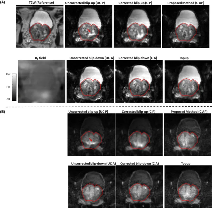
FIGURE 3 In vivo patient 1 reconstruction results for b‐value of 0 and b‐value of 500 s/mm2 are shown in (a) and (b), respectively. The reference T2W image and estimated B0 field (in Hz) are shown in (a). For EPI scans, the AP axis was selected as the phase‐encoding direction with fat shift in the direction “P” for blip‐up and “A” for blip‐down scans, respectively. Whole prostate (red) was delineated on reference T2W image and overlaid on reconstructions without distortion correction (uncorrected blip‐up [UC P] and uncorrected blip‐down [UC A]), reconstruction with distortion correction using data from 1 direction only (corrected blip‐up [C P] and corrected blip‐down [C A]), model‐based reconstruction using both blip‐up and blip‐down data (C AP), and Topup method (Topup). Red arrows indicate the regions of pile‐up. The proposed method corrected most of the signal pileup and has better resolution details than the Topup method
1 and 25 for patient 1) that had significant different phases in conjugate phase reconstructions. Without phase correction, signal cancellation occurred in the reconstructed image in each diffusion direction. By using the proposed phase correc-tion (Equacorrec-tion 8), the signal was preserved in each diffusion direction. The magnitude average of the reconstructions in three diffusion directions (Mag Avg) is shown in the right column that had close correspondence to the reference T2W image.
4
|
DISCUSSION
A novel model‐based reconstruction framework is pro-posed that can correct for geometric distortions, signal pileup, and signal dropout in diffusion‐weighted prostate images. By using the power of complimentary encoding information within data from both blip‐up and blip‐down directions, the model‐based framework was able to cor-rect most of the pileup in regions of severe distortions and
FIGURE 4 In vivo patient 2 reconstruction results for b‐value of 0 and b‐value of 500 s/mm2 are shown in (a) and (b), respectively. The reference T2W image and estimated B0 field (in Hz) are shown in (a). For EPI scans, the AP axis was selected as the phase‐encoding direction with fat shift in the direction “P” for blip‐up and “A” for blip‐down scans, respectively. Whole prostate (red) was delineated on reference T2W and overlaid on reconstructions without distortion correction (uncorrected blip‐up [UC P] and uncorrected blip‐down [UC A]), reconstruction with distortion correction using data from 1 direction only (corrected blip‐up [C P] and corrected blip‐down [C A]), model‐based reconstruction using both blip‐up and blip‐down data (C AP), and Topup method (Topup). The proposed method performed better than all other reconstructions in terms of distortion correction
performed better than the Topup method (commonly used for neuroimaging) or model‐based reconstructions using data from 1 phase‐encoding gradient direction only. The proposed mutual information maximization used for cor-rection of center frequency offset in the B0 field may also
be used as a method for overcoming uncertainties in coor-dinates that may happen in the process of reconstruction from raw data.
The proposed method assumes the B0 field to be static
except for center frequency offset attributed to the frequency drift between B0 and EPI scans. In case of motion or changes
in the rectal area adjacent to the prostate region between the EPI and B0 scans, the B0 field estimated from B0 scan may
be mismatched, resulting in inaccurate distortion correction. Some of the remaining distortions in the proposed method reconstructions can be attributed to dynamic changes in B0 FIGURE 5 In vivo reconstruction results for selected patients (P4, P6, and P9) for data acquired at b‐value of 0 s/mm2. For EPI scans, the AP axis was selected as the phase‐encoding direction with fat shift in the direction “P” for blip‐up and “A” for blip‐down scans, respectively. Whole prostate (red) was delineated on a reference T2W image (left column) and overlaid on uncorrected blip‐up (UC P), uncorrected blip‐down (UC A), Topup, and proposed distortion‐corrected (C AP) reconstructions
FIGURE 6 In vivo reconstruction results for selected patients (P4, P6, and P9) for data acquired at b‐value of 500 s/mm2. For EPI scans, the AP axis was selected as the phase‐encoding direction with fat shift in the direction “P” for blip‐up and “A” for blip‐down scans, respectively. Whole prostate (red) was delineated on a reference T2W image (left column) and overlaid on uncorrected blip‐up (UC P), uncorrected blip‐down (UC A), Topup, and proposed distortion‐corrected (C AP) reconstructions
field because no antispasmodic agent drug was administered in our scans that would suppress bowel movements and/or rectal gas. Changes in B0 might be addressed by a joint
esti-mation of both B0 and the corrected EPI images, starting with
the initial B0 fields estimated from B0 scan.30
For higher b‐values (b‐value > = 1000 s/mm2), the low
SNR in the reconstructed images might affect the inverse problem and the technique may benefit from preconditioning or additional regularization.
Our proposed method uses a B0 field estimated from a
dual‐echo gradient echo scan. In image regions where the individual echoes have low SNR or missing signal (espe-cially in the rectal‐air region), the measurement of B0 field
in that area might not be always possible, leading to noisy and unwrapped phases in the B0 field. To address this issue,
B0 field might be modeled in this region using a
suscep-tibility map distribution31 that could be obtained from a
segmentation of air and tissue areas on a reference T2W
image. Alternatively, a projection onto dipole fields (PDF) method32 might also be used for estimating the B
0 field
in-side the rectal‐air region. The PDF method calculates the B0 field inside an ROI by projection of known dipole fields
from outside the ROI.
Last, the proposed method does not include any physio-logical motion effects that may occur between the EPI blip‐ up and blip‐down scans. In case of motion between blip‐up and blip‐down scans, both motion parameters and the image would need to be estimated simultaneously and the optimi-zation in Equation 10 becomes nonconvex. The optimioptimi-zation may be simplified by estimating motion in a preceding step similar to the framework in a previous work33 by
register-ing model‐based reconstructions from blip‐up and blip‐down scans with either blip‐up or blip‐down reconstruction being set as the reference. The estimated motion fields can then be incorporated into Equation 10 by motion matrix transfor-mation17,33 that will relate the acquired corrupted k‐space FIGURE 7 Quantitative assessment: box plots showing Dice scores (range, 0–1) for uncorrected blip‐up (UC P), uncorrected blip‐down (UC A), Topup, and proposed method (C AP) corresponding to b‐value of 0 s/mm2 (b
0) and b‐value of 500 s/mm2 (b500) in the left and right columns, respectively. The T2W image was taken as a reference for calculation of Dice scores
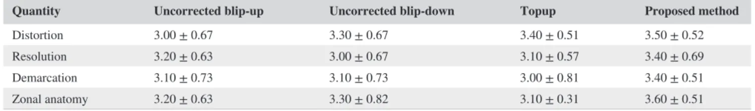
TABLE 1 Qualitative scores across 10 patients for different reconstruction methods for data acquired at b‐value of 0 s/mm2
Quantity Uncorrected blip‐up Uncorrected blip‐down Topup Proposed method
Distortion 3.00 ± 0.67 3.30 ± 0.67 3.40 ± 0.51 3.50 ± 0.52
Resolution 3.20 ± 0.63 3.00 ± 0.67 3.10 ± 0.57 3.40 ± 0.69
Demarcation 3.10 ± 0.73 3.10 ± 0.73 3.00 ± 0.81 3.40 ± 0.51
Zonal anatomy 3.20 ± 0.63 3.30 ± 0.82 3.10 ± 0.31 3.60 ± 0.51
The associated standard deviations are also indicated.
TABLE 2 Qualitative scores across 10 patients for different reconstruction methods for data acquired at b‐value of 500 s/mm2
Quantity Uncorrected blip‐up Uncorrected blip‐down Topup Proposed method
Distortion 3.30 ± 0.67 3.40 ± 0.70 3.50 ± 0.52 3.90 ± 0.57
Resolution 3.00 ± 0.47 3.10 ± 0.74 3.00 ± 0.47 3.20 ± 0.78
Demarcation 3.30 ± 0.67 3.30 ± 0.48 3.50 ± 0.84 3.50 ± 0.52
Zonal anatomy 3.10 ± 0.56 2.80 ± 0.63 3.10 ± 0.56 3.10 ± 0.73
data to corrected images through a combined model that is a concatenation of B0 distortion and motion corruption
effects.
Prostate diffusion MRI is recognized as a potential bio-marker for tumor detection, but, currently, it is unusable in some patients because of significant distortions. We proposed a novel model‐based reconstruction framework that can cor-rect these distortions by using data from opposite phase‐en-coding gradient directions. The proposed method was applied successfully in 10 clinical patients, despite no antispasmodic drug being administered. The proposed technique may offer potential to radiologists and clinicians by increasing the
diagnostic value of prostate images for tumor detection, thus making prostate MRI a more reliable and reproducible bio-marker in future.
ACKNOWLEDGMENTS
We acknowledge research support provided by Philips Healthcare.
ORCID
David Atkinson http://orcid.org/0000-0003-1124-6666
FIGURE 8 Evaluation of phase correction procedure: model‐based reconstruction with and without phase correction for dynamic frames of data acquired at b‐value of 500 s/mm2. Reconstructions for each individual diffusion direction (Dir 1, Dir 2, and Dir 3) are shown for patient 11 and patient 1 in (a) and (b), respectively. Data are combined from 2 dynamics (dynamic 1 and 13 for patient 11, dynamic 1 and 25 for patient 1) that had significantly different phases in conjugate phase reconstructions. Without phase correction, the phase cancellation in each model‐based reconstruction leads to signal dropout and signal cancellations (bottom row in a and b). The proposed phase correction procedure preserved signal in each diffusion direction (top row in a and b). The magnitude average (Mag avg) of model‐based reconstructions from the 3 directions (Dir 1, Dir 2, and Dir 3) is shown in the right column
REFERENCES
1. Murphy G, Haider M, Ghai S, Sreeharsha B. The expanding role of MRI in prostate cancer. Am J Roentgenol. 2013;201:1229–1238. 2. Shimofusa R, Fujimoto H, Akamata H, et al. Diffusion‐
weighted imaging of prostate cancer. J Comput Assist Tomogr. 2005;29:149–153.
3. Miao H, Fukatsu H, Ishigaki T. Prostate cancer detection with 3‐T MRI: comparison of diffusion‐weighted and T2‐weighted imag-ing. Eur J Radiol. 2007;61:297–302.
4. Steiger P, Thoeny HC. Prostate MRI based on PI‐RADS version 2: how we review and report. Cancer Imaging. 2016;16:9. 5. Kayhan A. Multi‐parametric MR imaging of transition zone
prostate cancer: imaging features, detection and staging. World J Radiol. 2010;2:180–187.
6. Donato F, Costa DN, Yuan Q, Rofsky NM, Lenkinski RE, Pedrosa I. Geometric distortion in diffusion‐weighted MR imaging of the prostate‐contributing factors and strategies for improvement.
Acad Radiol. 2014;21:817–823.
7. Gill AB, Czarniecki M, Gallagher FA, Barrett T. A method for mapping and quantifying whole organ diffusion‐weighted image distortion in MR imaging of the prostate. Sci Rep. 2017;7: 12727.
8. Andersson JL, Skare S, Ashburner J. How to correct suscepti-bility distortions in spin‐echo echo‐planar images: application to diffusion tensor imaging. Neuroimage. 2003;20:870–888. 9. Robson MD, Gore JC, Constable RT. Measurement of the point
spread function in MRI using constant time imaging. Magn Reson Med. 1997;38:733–740.
10. Reber PJ, Wong EC, Buxton RB, Frank LR. Correction of off res-onance‐related distortion in echo‐planar imaging using EPI‐based field maps. Magn Reson Med. 1998;39:328–330.
11. Jezzard P, Balaban RS. Correction for geometric distortion in echo planar images from B0 field variations. Magn Reson Med. 1995;34:65–73.
12. Munger P, Greller GR, Peters TM, Pike GB. An inverse prob-lem approach to the correction of distortion in EPI images. IEEE Trans Med Imaging. 2000;19:681–689.
13. Holland D, Kuperman JM, Dale AM. Efficient correction of inho-mogeneous static magnetic field‐induced distortion in echo planar imaging. Neuroimage. 2010;50:175–183.
14. In MH, Posnansky O, Beall EB, Lowe MJ, Speck O. Distortion correction in EPI using an extended PSF method with a reversed phase gradient approach. PLoS One. 2015;10:e0116320. 15. Kale SC, Lerch JP, Henkelman RM, Chen XJ. Optimization of the
SNR‐resolution tradeoff for registration of magnetic resonance images. Hum Brain Mapp. 2008;29:1147–1158.
16. Kale SC, Chen XJ, Henkelman RM. Trading off SNR and resolu-tion in MR images. NMR Biomed. 2009;22:488–494.
17. Batchelor PG, Atkinson D, Irarrazaval P, Hill DL, Hajnal J, Larkman D. Matrix description of general motion correc-tion applied to multishot images. Magn Reson Med. 2005;54: 1273–1280.
18. Newbould R, Skare S, Bammer R. On the utility of complex‐aver-aged diffusion‐weighted images. ISMRM. 2008;16:1810. https:// cds.ismrm.org/ismrm-2008/files/01810.pdf. Accessed October 10, 2018.
19. Skare S, Holdsworth S. On the battle between Rician noise and phase‐interferences in DWI. ISMRM. 2009;12:1409. https://ar-chive.ismrm.org/2009/1409.html. Accessed October 10, 2018.
20. Scott AD, Nielles‐Vallespin S, Ferreira PF, McGill LA, Pennell DJ, Firmin DN. The effects of noise in cardiac diffusion ten-sor imaging and the benefits of averaging complex data. NMR Biomed. 2016;29:588–599.
21. Lauzon CB, Crainiceanu C, Caffo BC, Landman BA. Assessment of bias in experimentally measured diffusion tensor imaging pa-rameters using SIMEX. Magn Reson Med. 2013;69:891–902. 22. Pruessmann KP, Weiger M, Scheidegger MB, Boesiger P.
SENSE: sensitivity encoding for fast MRI. Magn Reson Med. 1999;42:952–962.
23. Cover TM, Thomas JA. Elements of Information Theory. Hoboken, NJ: John Wiley & Sons; 2005.
24. Quantitative Susceptibility Mapping Toolbox. Cornell MRI Research Laboratory. http://weill.cornell.edu/mri/pages/qsm. html. Accessed April 28, 2018.
25. Garcia D. Robust smoothing of gridded data in one and higher dimensions with missing values. Comput Stat Data Anal. 2010;54:1167–1178.
26. Lagarias JC, Reeds JA, Wright MH, Wright PE. Convergence properties of the Nelder‐Mead simplex method in low dimen-sions. SIAM J Optim. [Internet]. 1998;9:112–147.
27. The Horos Project, version 1.1.7. https://horosproject.org/ li-censed under the GNU Lesser General Public License, Version 3.0 (LGPL 3.0). Access June 27, 2018.
28. Dice LR. Measures of the amount of ecologic association be-tween species. Ecology. 1945;26:297–302.
29. Stocker D, Manoliu A, Becker AS, et al. Image quality and geometric distortion of modern diffusion‐weighted imaging se-quences in magnetic resonance imaging of the prostate. Invest Radiol. 2018;53:200–206.
30. Ramani S, Fessler JA. Parallel MR image reconstruction using augmented lagrangian methods. IEEE Trans Med Imaging. 2011;30:694–706.
31. Jordan CD, Daniel BL, Koch KM, Yu H, Conolly S, Hargreaves BA. Subject‐specific models of susceptibility‐induced B0 field variations in breast MRI. J Magn Reson Imaging. 2013;37:227–232.
32. Liu T, Khalidov I, de Rochefort L, et al. A novel background field removal method for MRI using projection onto dipole fields (PDF). NMR Biomed. 2011;24:1129–1136.
33. Usman M, Atkinson D, Odille F, et al. Motion corrected com-pressed sensing for free‐breathing dynamic cardiac MRI. Magn Reson Med. 2013;70:504–516.
SUPPORTING INFORMATION
Additional supporting information may be found online in the Supporting Information section at the end of the article.
FIGURE S1 In vivo reconstruction results for patients 3 (P3) to patient 10 (P10) for data acquired at b‐value of 0. For EPI scans, the AP axis was selected as the phase‐encoding direc-tion with fat shift in the direcdirec-tion “P” for blip‐up and “A” for blip‐down scans, respectively. Whole prostate (red) was delineated on reference T2W image (left column) and over-laid on uncorrected blip‐up (UC P), uncorrected blip‐down (UC A), Topup, and proposed distortion‐corrected (C AP) reconstructions
APPENDIX 1
The mutual information function MI(A,B)23 between the 2
images A and B, is defined as:
where H(A) and H(B) are marginal entropy functions for im-ages A and B, respectively, given as:
Pa being the probability of pixels in image A having signal intensity a and Pb being the probability of pixels in image B having signal intensity b.
H(A, B) is the joint entropy function of images A and B calculated as:
Pab being the joint probability of pixels in image A having
intensity a and pixels in image B having intensity b MI(A,B) =H(A) +H(B) −H(A,B) H(A) = −∑ a PalogPa⋅ ⋅ ⋅ ⋅and⋅ ⋅ ⋅ ⋅H(B) = − ∑ b PblogPb H(A,B) = −∑ a ∑ b PablogPab FIGURE S2 In vivo reconstruction results for patients 3 (P3)
to patient 10 (P10) for data acquired at b‐value of 500 s/mm2.
For EPI scans, the AP axis was selected as the phase‐encod-ing direction with fat shift in the direction “P” for blip‐up and “A” for blip‐down scans, respectively. Whole prostate (red) was delineated on reference T2W image (left column) and overlaid on uncorrected blip‐up (UC P), uncorrected blip‐ down (UC A), Topup, and proposed distortion‐corrected (C AP) reconstructions
FIGURE S3 Plot of normalized residual error r=E
H
Ex−EHỸ2
EHỸ
2 as a function of the CG iteration number
FIGURE S4 Qualitative assessment: mean percentage of im-provement in qualitative scores (distortion, resolution, demar-cation, and zonal anatomy) using model‐based reconstruction compared to uncorrected blip‐up (UC P), uncorrected blip‐ down (UC‐A), and Topup methods. The results are shown for b‐values of 0 and 500 s/mm2. The improvements in all
the qualitative scores for the proposed method were positive compared to the other reconstructions
How to cite this article: Usman M, Kakkar L, Kirkham A, Arridge S, Atkinson D. Model‐based reconstruction framework for correction of signal pile‐up and geometric distortions in prostate diffusion MRI. Magn
Reson Med. 2019;81:1979–1992. https://doi.