BANCO CENTRAL DE RESERVA DEL PERÚ
Oil Shocks and Optimal Monetary Policy
Carlos Montoro*
* Banco Central de Reserva del Perú and LSE
DT. N° 2007-010
Serie de Documentos de Trabajo
Working Paper series
Agosto 2007
Los puntos de vista expresados en este documento de trabajo corresponden a los del autor y no reflejan necesariamente la posición del Banco Central de Reserva del Perú.
The views expressed in this paper are those of the author and do not reflect necessarily the position of the Central Reserve Bank of Peru.
Oil Shocks and Optimal Monetary Policy
∗ Carlos Montoro†Banco Central de Reserva del Per´u and LSE First version: November 2005
This version: June 2007
Abstract
This paper investigates how monetary policy should react to oil shocks in a micro-founded model with staggered price-setting and oil as a non-produced input in the pro-duction function. We extend Benigno and Woodford (2005) to obtain a second order approximation to the expected utility of the representative household when the steady state is distorted and the economy is hit by oil price shocks.
The main result is that oil price shocks generate a trade-off between inflation and output stabilisation when oil has low substitutability in production. Therefore, it becomes optimal to the monetary authority to stabilise partially the effects of oil shocks on inflation and some inflation is desirable. We also find, in contrast to Benigno and Woodford (2005), that this trade-off remains even when we eliminate the effects of monopolistic distortions from the steady state.
Our results also shed light on how technological improvements which reduces the de-pendence on oil, also reduce the impact of oil shocks on the economy. This can explain why oil shocks have lower impact on inflation in the 2000s in contrast to the 1970s. Since oil has become easier to substitute with other renewable resources, the impact of oil shocks has been dampened.
JEL Classification: D61, E61.
Keywords: Optimal Monetary Policy, Welfare, Second Order Solution, Oil Price Shocks, Endogenous Trade-off.
∗
I would like to thank Chris Pissarides, Gianluca Benigno, Pierpaolo Benigno, John Driffill and participants at the Macroeconomics Student Seminar at LSE and the BCRP for their comments and help. The views expressed herein are those of the author and do not necessarily reflect those of the Banco Central de Reserva del Per´u. Any errors are my own responsibility.
†
1
Introduction
Oil is an important production factor in economic activity, because every industry uses it to some extent. Moreover, since oil cannot easily be substituted by other production factors, economic activity is heavily dependent on its use. Furthermore, the oil price is determined in a weakly competitive market; there are few large oil producers dominating the world market, setting its price above a perfect competition level. Also, its price fluctuates considerably due to the effects of supply and demand shocks in this market1.
The heavy dependence on oil and the high volatility of its price generates a concern among the policymakers on how to react to oil shocks. Oil shocks have serious effects on the economy because they raise prices for an important production input and for important consumer goods (gasoline and heating oil). This causes an increase in inflation and subsequently a decrease in output, generating also a dilemma for policymaking. On one hand, if monetary policy makers focus exclusively on the recessive effects of oil shocks and try to stabilise output, this would generate inflation. On the other hand, if monetary policy makers focus exclusively on neutralising the impact of the shock on inflation through a contractive monetary policy, some sluggishness in the response of prices to changes in output would imply large reductions in output. Therefore, policymakers are confronted with a trade-off between stabilising inflation and output. But, what exactly should be the optimal stabilisation of inflation and output? Which factors affect this trade-off? To our knowledge there is not been a formal study on this topic.
To answer these questions we extend the literature on optimal monetary policy including oil in the production process in a standard New Keynesian model. In doing so, we extend Benigno and Woodford (2005) to obtain a second-order approximation to the expected utility of the representative household when the steady state is distorted and the economy is hit by oil price shocks. We include oil as a non-produced input as in Blanchard and Gali (2005), but differently from those authors we use a constant-elasticity-of-substitution (CES) production function to capture the low substitutability of oil. Then, a low elasticity of substitution between labour and oil indicates a high dependence on oil2.
The analysis of optimal monetary policy in microfounded models with staggered price set-ting using a quadratic welfare approximation was first introduced by Rotemberg and Woodford (1997) and expounded by Woodford (2003) and Benigno and Woodford (2005). This method allows us to obtain a linear policy rule derived from maximising the quadratic approximation of the welfare objective subject to the linear constraints that are first-order approximations of the true structural equations. This methodology is called linear-quadratic (LQ). The advantage of this approach is that it allows us to characterise analytically how changes in the produc-tion funcproduc-tion and in the oil shock process affect the monetary policy problem. Moreover, in contrast to the Ramsey policy methodology, which also allows a correct calculation of a linear
1
For example during the 1970s and through the 1990s most of the oil shocks seemed clearly to be on the international supply side, either because of attempts to gain more oil revenue or because of supply interruptions, such as the Iranian Revolution and the first Gulf war. In contrast, in the 2000s the high price of oil is more related to demand growth in the USA, China, India and other countries.
2
In contrast, Blanchard and Gali (2005) use a Cobb-Douglas production function, in which the elasticity of substitution is equal to one.
approximation of the optimal policy rule, the LQ approach is useful to evaluate not only the optimal rules, but also to evaluate and rank sub-optimal monetary policy rules.
A property of standard New Keynesian models is that stabilising inflation is equivalent to stabilising output around some desired level, unless some exogenous cost-push shock dis-turbances are taken into account. Blanchard and Gali (2005) called this feature the ”divine coincidence”. These authors argue that this special feature comes from the absence of non-trivial real imperfections, such as real wage rigidities. Similarly, Benigno and Woodford (2004, 2005) show that this trade-off also arises when the steady state of the model is distorted and there are government purchases in the model.
We found that, when oil is introduced as a low-substitutable input in a New Keynesian model, a trade-off arises between stabilising inflation and the gap between output and some desired level. We call this desired level the “‘efficient level”. In this case, because output at the efficient level fluctuates less than it does at the natural level, it becomes optimal to the monetary authority to react partially to oil shocks and therefore, some inflation is desirable. Moreover, in contrast to Benigno and Woodford (2005), this trade-off remains even when the effects of the monopolistic distortions are eliminated from the steady state.
This trade-off is generated because oil shocks affect output and labour differently, generat-ing a wedge between the effects on the utility of consumption and the disutility of labour. The lower the elasticity of substitution in production, the higher this wedge and also the greater the trade-off. In contrast, in the case of a Cobb-Douglas production function, there is no such a trade-off because this wedge is zero. Then, in the Cobb-Douglas case stabilising output around the natural level also implies stabilising output around its efficient level.
Also, the substitutability among production factors affects both the weights on the two stabilisation objectives and the definition of the welfare-relevant output gap. The lower the elasticity of substitution, the higher the cost-push shock generated by oil shocks and the lower the weight on output stabilisation relative to inflation stabilisation. Moreover, when the share of oil in the production function is higher, or the steady-state oil price is higher, the size of the cost-push shock increases.
Section 2 presents our New Keynesian model with oil prices in the production function. Section 3 includes a linear quadratic approximation to the policy problem. Section 4 uses the linear quadratic approximation to the problem to solve for the different rules of monetary policy and make some comparative statics to the parameters related to oil. The last section concludes.
2
A New Keynesian model with oil prices
The model economy corresponds to the standard New Keynesian Model in the line of Clarida et.al. (2000). In order to capture oil shocks we follow Blanchard and Gali (2005) by introducing a non-produced input M, represented in this case by oil. Q will be the real price of oil which is assumed to be exogenous. This model is similar to the one used by Castillo et.al. (2007), except that we additionally include taxes on sales of intermediate goods and oil to analyse the distortions in steady state.
2.1 Households
We assume the following utility function on consumption and labour of the representative consumer Uto =Eto ∞ X t=to βt−to Ct1−σ 1−σ − L1+t ν 1 +ν (2.1)
whereσrepresents the coefficient of risk aversion andν captures the inverse of the elasticity of labour supply. The optimiser consumer takes decisions subject to a standard budget constraint which is given by Ct= WtLt Pt +Bt−1 Pt − 1 Rt Bt Pt +Γt Pt + Tt Pt (2.2)
whereWtis the nominal wage,Ptis the price of the consumption good,Btis the end of period nominal bond holdings, Rt is the nominal gross interest rate , Γt is the share of the represen-tative household on total nominal profits, andTtare net transfers from the government3. The first order conditions for the optimising consumer’s problem are:
1 =βEt " Rt Pt Pt+1 Ct+1 Ct −σ# (2.3) Wt Pt =CtσLνt =M RSt (2.4)
Equation (2.3) is the standard Euler equation that determines the optimal path of consump-tion. At the optimum the representative consumer is indifferent between consuming today or tomorrow, whereas equation (2.4) describes the optimal labour supply decision. M RStdenotes for the marginal rate of substitution between labour and consumption. We assume that labour markets are competitive and also that individuals work in each sector z∈[0,1]. Therefore,L
corresponds to the aggregate labour supply:
L=
Z 1
0
Lt(z)dz (2.5)
2.2 Firms
2.2.1 Final Good Producers
There is a continuum of final good producers of mass one, indexed by f ∈[0,1] that operate in an environment of perfect competition. They use intermediate goods as inputs, indexed by
z∈[0,1] to produce final consumption goods using the following technology:
Ytf = Z 1 0 Yt(z) ε−1 ε dz ε−ε1 (2.6) 3
In the model we assume that the government owns the oil endowment. Oil is produced in the economy at zero cost and sold to the firms at an exogenous priceQt.The government transfers all the revenues generated
whereεis the elasticity of substitution between intermediate goods. Then the demand function of each type of differentiated good is obtained by aggregating the input demand of final good producers Yt(z) = Pt(z) Pt −ε Yt (2.7)
where the price level is equal to the marginal cost of the final good producers and is given by:
Pt= Z 1 0 Pt(z)1−εdz 1−1ε (2.8)
and Yt represents the aggregate level of output.
Yt=
Z 1
0
Ytfdf (2.9)
2.2.2 Intermediate Goods Producers
There is a continuum of intermediate good producers. All of them have the following CES production function Yt(z) = h (1−α) (Lt(z)) ψ−1 ψ +α(M t(z)) ψ−1 ψ iψψ−1 (2.10)
whereM is oil which enters as a non-produced input, ψ represents the intratemporal elasticity of substitution between labour-input and oil and α denotes the share of oil in the production function. We use this generic production function in order to capture the fact that oil has few substitutes, in general we assume that ψ is lower than one. The real oil price,Qt, is assumed to follow anAR(1) process in logs,
logQt= logQ+ρlogQt−1+εt (2.11)
whereQ is the steady state level of oil price. From the cost minimisation problem of the firm we obtain an expression for the real marginal cost given by:
M Ct(z) = " (1−α)ψ Wt Pt 1−ψ +αψ((1 +τq)Qt)1−ψ #1−1ψ (2.12)
whereM Ct(z) represents the real marginal cost,Wt nominal wages andPtthe consumer price index, and τq is a proportional tax on oil sales. Notice that marginal costs are the same for all intermediate firms, since technology has constant returns to scale and factor markets are competitive, i.e. M Ct(z) =M Ct. On the other hand, the individual firm’s labour demand is given by: Ldt(z) = 1 1−α Wt/Pt M Ct −ψ Yt(z) (2.13)
Intermediate producers set prices following a staggered pricing mechanism a la Calvo. Each firm faces an exogenous probability of changing prices given by (1−θ). A firm that changes its price in period t chooses its new price Pt(z) to maximise:
Et ∞ X k=0 θkζt,t+kΓ (Pt(z), Pt+k, M Ct+k, Yt+k) whereζt,t+k=βk C t+k Ct −σ Pt
Pt+k is the stochastic discount factor. The function: Γ (P(z), P, M C, Y) = [(1−τy)P(z)−P M C] P(z) P −ε Y
is the after-tax nominal profits of the supplier of good zwith price Pt(z),when the aggregate demand and aggregate marginal costs are equal to Y and M C, respectively. τy is the propor-tional tax on sale revenues, which we assume constant and equal to τy.The optimal price that
solves the firm’s problem is given by
Pt∗(z) Pt = µEt ∞ P k=0 θkζt,t+kM Ct,t+kFtε++1kYt+k Et ∞ P k=0 θkζ t,t+kFtε+kYt+k (2.14)
where µ ≡ ε−ε1/(1−τy) is the price markup, P∗
t (z) is the optimal price level chosen by the firm andFt+k= PtP+tk the cumulative level of inflation. The optimal price solves equation (2.14) and is determined by the average of expected future marginal costs as follows:
Pt∗(z) Pt =µEt "∞ X k=0 ϕt,t+kM Ct,t+k # (2.15) where ϕt,t+k = θkζt,t+kFtε++1kYt+k Et ∞ P k=0 θkζ t,t+kFtε+kYt+k (2.16)
Since only a fraction (1−θ) of firms changes prices every period and the remaining one keeps its price fixed, the aggregate price level, the price of the final good that minimise the cost of the final goods producers, is given by the following equation:
Pt1−ε=θPt1−−1ε+ (1−θ) (Pt∗(z))1−ε (2.17) Following Benigno and Woodford (2005), equations (2.14) and (2.17) can be written recursively introducing the auxiliary variables Nt andDt (see appendix B for details on the derivation):
θ(Πt)ε−1= 1−(1−θ)
Nt1−
Dt=Yt(Ct)−σ+θβEt h (Πt+1)−1Dt+1 i (2.19) Nt=µYt(Ct)−σM Ct+θβEt[(Πt+1)Nt+1] (2.20) Equation (2.18) comes from the aggregation of individual firms prices. The ratioNt/Dt repre-sents the optimal relative price Pt∗(z)/Pt.These three last equations summarise the recursive representation of the non linear Phillips curve.
2.3 Market Clearing
In equilibrium labour, intermediate and final goods markets clear. Since there is neither capital accumulation nor government sector, the economy-wide resource constraint is given by
Yt=Ct (2.21)
The labour market clearing condition is given by:
Lst =Ldt (2.22)
Where the demand for labour comes from the aggregation of individual intermediate producers in the same way as for the labour supply:
Ld = Z 1 0 Ldt(z)dz= 1 1−α Wt/Pt M Ct −ψZ 1 0 Yt(z)dz (2.23) Ld = 1 1−α Wt/Pt M Ct −ψ Yt∆t where ∆t= R1 0 P t(z) Pt −ε
dz is a measure of price dispersion. Since relative prices differ across firms due to staggered price setting, input usage will differ as well, implying that is not possible to use the usual representative firm assumption. Therefore, the price dispersion factor, ∆t appears in the aggregate labour demand equation. We can also use (2.17) to derive the law of motion of ∆t ∆t= (1−θ) 1−θ(Πt)ε−1 1−θ !ε/(ε−1) +θ∆t−1(Πt)ε (2.24)
Note that inflation affects welfare of the representative agent through the labour market. From (2.24) we can see that higher inflation increases price dispersion and from (2.23) that higher price dispersion increases the labour amount necessary to produce certain level of output, implying more disutility on (2.1).
2.4 Monetary Policy
We abstract from any monetary frictions assuming that the central bank can control directly the risk-less short-term interest rateRt.
2.5 The Log Linear Economy
To illustrate the effects of oil in the dynamic equilibrium of the economy, we take a log linear approximation of equations (2.1), (2.4),(2.11),(2.12),(2.18),(2.19),(2.20) and (2.23) around the deterministic steady-state. We denote variables in steady state with over bars (i.e. X) and their log deviations around the steady state with lower case letters (i.e. xt= log(XXt)). After, imposing the goods and labour market clearing conditions to eliminate real wages and labour from the system, the dynamics of the economy is determined by the following equations,
lt=yt−δ[(σ+v)yt−qt] (2.25) mct=χ(ν+σ)yt+ (1−χ)qt (2.26) πt=βEtπt+1+κmct (2.27) yt=Etyt+1− 1 σ(rt−Etπt+1) (2.28) qt=ρqt−1+ξt (2.29) where α ≡ αψ (1+τq)Q M C 1−ψ , δ ≡ ψχ1−αα, χ ≡ 1−α 1+vψα and κ ≡ 1−θ θ (1−θβ) . Q, and
M C represent the steady-state value of oil prices and of the marginal cost, respectively. α
corresponds to the share of oil on marginal costs in steady state, δ and (1−χ) accounts for the effects oil prices in labour and marginal costs, respectively; andκis the elasticity of inflation respect to marginal costs.
Interestingly, the effects of oil prices on marginal costs, equation (2.26), depends crucially on the share of oil in the production function, α, and on the elasticity of substitution between oil and labour,ψ. Thus, whenαis large,χis smaller making marginal costs more responsive to oil prices. Also, whenψis lower, the impact of oil on marginal costs is larger. It is important to note that even though the share of oil in the production function,α,can be small, its impact on marginal cost, α, can be magnified when oil has few substitutes (that is when ψ is low). Moreover, a permanent increase in oil prices, that is an increase in Q, would make marginal cost of firms more sensitive to oil price shocks since it increasesα. In the case that α= 0, the model collapses to a standard close economy New Keynesian model without oil.
If we replace equation (2.26) in (2.27) we obtain the traditional New Keynesian Phillips curve.
πt=κyyt+κqqt+βEtπt+1 (2.30) where κy = κχ(v+σ) and κq = κ(1−χ). We define the natural rate of output as the level of output such inflation is zero in all periods, this is given by ynt =−κq
κyqt. Then, the Phillips curve can be written in terms of deviations of output from its natural level:
2.6 Distortions in steady state
The details of the steady state of the variables is in appendix A. In steady state we have two distortions: the first one is the monopolistic distortion and the second one comes from the Oil market. Related to the first distortion, because intermediate goods producers set prices monopolistically, the price they charge is higher than the marginal cost, and the monopolistic distortion is given by:
M C = 1−τ
ε/(ε−1) = 1
µ ≤1 (2.31)
whereτ =τq. Let’s denote the steady state distortion caused by monopolistic competition by
Φ = 1− 1−τ
ε/(ε−1)
where Φ measures the monopolistic distortion, when taxes on sales can eliminate this distortion we have that Φ = 0. In a competitive equilibrium the marginal rate of substitution between consumption and leisure must equal the marginal product of labour. However, monopolistic distortions generates a wedge between this two, given by ΦL
ΦL = 1− VL UC ∂L ∂Y (2.32) = 1−(1−α) (1−Φ) (1−δ(σ+v))
Note that in this economy since labour is not the only input in the production function, then ΦL 6= Φ the wedge in the labour market is not the same as the distortion in marginal costs. Also, eliminating the monopolistic distortion (Φ) doesn’t eliminate this wedge. The effect of the monopolistic distortion on ΦL can be eliminated with a subsidy (negative tax rate) such that ΦL= 0.
Similarly, the oil market distortion affects the share of oil in the steady state marginal costs: α=αψ 1 +τ Q Q M C !1−ψ
Since in this economy firms are price takers for oil, its price can also be distorted from a competitive equilibrium. Again, this distortion can be eliminated with a tax (or subsidy) such that 1 +τQQ/M C equals to the one from a competitive equilibrium. In general, when the oil price is to high respect to marginal cost, the policy to eliminate this distortion is to subsidise the use of oil (τq<0), since such high price increases the costs of firms and reduces output and consumption below the optimal.
3
A Linear-Quadratic Approximate Problem
In this section we present a second order approximation of the welfare function of the repre-sentative household as function of purely quadratic terms. This representation allows us to characterise the policy problem using only a linear approximation of the structural equations of the model and also to rank sub-optimal monetary policy rules.
Since the model has a distorted steady state, a standard second order Taylor approximation of the welfare function will include linear terms, which would lead to an inaccurate approx-imation of the optimal policy in a linear-quadratic approach. We use then the methodology proposed by Benigno and Woodford (2005), which consists on eliminating the linear terms of the policy objective using a second order approximation of the aggregate supply.
3.1 Second order Taylor expansion of the model
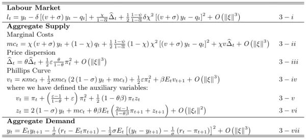
In this sub-section we present a log-quadratic (Taylor-series) approximation of the fundamental equations of the model around the steady state, a detailed derivation is provided in Appendix B. The second-order Taylor-series expansion serves to compute the equilibrium fluctuations of the endogenous variables of the model up to a residual of order Okξk2, where kξtk is a bound on the size of the oil price shock. Up to second order, equations (2.25) to (2.28) are replaced by the following set of log-quadratic equations:
Labour Market lt=yt−δ[(v+σ)yt−qt] +1−χα∆bt+2111−−ψαδχ2[(v+σ)yt−qt]2+O kξk3 3−i Aggregate Supply Marginal Costs mct=χ(v+σ)yt+ (1−χ)qt+1211−−ψα(1−χ)χ2[(v+σ)yt−qt]2+χv∆bt+O kξk3 3−ii Price dispersion b ∆t=θ∆bt+12ε1−θθπ 2 t +O kξk 3 3−iii Phillips Curve vt=κmct+12κmct(2 (1−σ)yt+mct) +12επ2t +βEtvt+1+O kξk3 3−iv
where we have defined the auxiliary variables:
vt≡πt+ ε−1 1−θ+ε π2 t +12(1−θβ)πtzt 3−v zt≡2 (1−σ)yt+mct+θβEt 2ε−1 1−θβπt+1+zt+1 +O kξtk2 3−vi Aggregate Demand yt=Etyt+1−1σ(rt−Etπt+1)−12σEt (yt−yt+1)−σ1(rt−πt+1) 2 +O kξk3 3−vii
Table 3.1: Second order Taylor expansion of the equations of the model
Equations (3-i) and (3-ii) are obtained taking a second-order Taylor-series expansion of the aggregate labour and the real marginal cost equation, after using the labour market equilibrium to eliminate real wages. ∆bt is the log-deviation of the price dispersion measure ∆t, which is a
second order function of inflation (see appendix B for details) and its dynamic is represented with equation (3-iii).
We replace the equation for the marginal costs (3-ii) in the second order expansion of the Philips curve and iterate forward. Then, replace recursively the price dispersion terms from equation (3-iii) to obtain the infinite sum of the Phillips curve only as a function of output,
inflation and the oil shock: vto = ∞ X t=to βt−to κyyt+κqqt+12ε(1 +χv)π2t +12κ cyyyt2+ 2cyqytqt+cqqqt2 + (1−θ)χv∆bto−1+ kξtk3 (3.1)
wherecyy,cyq andcqq are defined in the appendix.
3.2 A second-order approximation to utility
A second order Taylor-series approximation to the utility function, expanding around the non-stochastic steady-state allocation is:
Uto =Y uc ∞ X t=to βt−to ΦLyt+ 1 2uyyy 2 t +uyqytqt+u∆∆bt +t.i.p.+Okξtk3 (3.2) where yt ≡ log Yt/Y
and ∆bt ≡ log ∆t measure deviations of aggregate output and the price dispersion measure from their steady state levels, respectively. The term ”t.i.p.” collects terms that are independent of policy (constants and functions of exogenous disturbances) and hence irrelevant for ranking alternative policies. ΦL is the wedge between the marginal rate of substitution between consumption and leisure and the marginal product of labour generated by the monopolistic distortion, defined in the previous section. The coefficients: uyy,uyq and
u∆ are defined in the appendix B.
We use equation (3-iii) to substitute in our welfare approximation the measure of price dispersion as a function of quadratic terms of inflation. Also, we use the second order approx-imation of the AS (equation 3.1) to solve for the infinite discounted sum of the expected level of output as function of purely quadratic terms. Then, as in Beningno and Woodford (2005) we replace this last expression in (3.2). We can rewrite (3.2) as:
Uto =−Ω " Eto ∞ X t=to βt−to 1 2λ(yt−y ∗ t)2+ 1 2π 2 t −Tto # +t.i.p.+Okξtk3 (3.3) where Ω = Y ucλπ and Tto = ΦL
κyvto, λπ is defined in the appendix. λ measures the relative weight between a welfare-relevant output gap and inflation. y∗t is the efficient output, the level of output that maximises our measure of welfare when inflation is zero. The values of λand
yt∗ are given by:
λ = κy ε (1−σψα)γ (3.4) yt∗ = − 1 +ψv σ+v α∗ 1−α∗ qt (3.5)
whereα∗ is the efficient share in steady state of oil in the marginal costs, given by:
α∗ = α
Both γ and η are function of the deep parameters of the model and are defined in the appendix. Note that the natural rate of output can be written in a similar way as the efficient output: ynt =− 1 +ψv σ+v α 1−α qt
3.3 The linear-quadratic policy problem
The policy objective Uto can be written on terms of inflation and the welfare-relevant output gap defined byxt:
xt≡yt−y∗t
Benigno and Woodford (2005) show that maximisation ofUto is equivalent to minimise the following lost functionLto subject to a predeterminated value of vto :
Lto ≡Eto ∞ X t=to βt−to 1 2λx 2 t + 1 2π 2 t (3.7)
Also, because the objective function is purely quadratic, a linear approximation of vto suffices to describe the initial commitments, given by vto =πto.
We are interested in evaluating monetary policy from a timeless perspective: optimising without regard of possible short run effects and avoiding possible time inconsistency problems. Then, from a timeless perspective the predetermined value ofπto must equal π
∗
to, the optimal value of inflation atto consistent with the policy problem. Thus, the policy objective consists on minimise (3.7) subject to the initial inflation rate:
πto =π ∗
to (3.8) and the Phillips curve for any date fromto onwards:
πt=κyxt+βEtπt+1+ut (3.9)
Note that we have expressed (3.9) in terms of the welfare relevant output gap, xt. ut is a ”cost-push” shock, that is proportional to the deviations in the real oil price:
ut ≡ κy(y∗t −ytn) = $qt where $≡κy 1 +ψv σ+v α 1−α − α∗ 1−α∗
In this model a ”cost-push” shock arises endogenously since oil generates a trade-off between stabilising inflation and deviations of output from an efficient level, different from the natural level. In the next section we characterise the conditions under which oil shocks preclude simultaneous stabilisation of inflation and the welfare-relevant output gap.
4
Optimal monetary response to oil shocks from a timeless
perspective.
In this section we use the linear-quadratic policy problem defined in the previous section to evaluate optimal and sub-optimal monetary policy rules under oil shocks. This policy problem can be summarised to maximise the following Lagrangian:
Lto ≡ −Eto P∞ t=toβ t−to1 2λx 2 t +12π 2 t −ϕt(πt−κyxt−βEtπt+1−ut) +ϕto−1 πto−π ∗ to (4.1) whereβt−toϕ
t is the Lagrange multiplier at period t.
The second order conditions for this problem are well defined for λ≥0, which is the case for plausible parameters of the model4. Then, as Benigno and Woodford (2005) show, since the loss function is convex, randomisation of monetary policy is welfare reducing and there are welfare gains when using monetary policy rules.
Under certain circumstances the optimal policy involves complete stabilisation of the infla-tion rate at zero for every period, that is complete price stability. These condiinfla-tions are related to how oil enters in the production function and are summarised in the following proposition:
Proposition 1 When the production function is Cobb-Douglas the efficient level of output is equivalent to the natural level of output.
In the case of a Cobb-Douglas production function, the elasticity of substitution between labour and oil is unity (i.e. ψ = 1). In this case η = 0 and the share of oil on the marginal costs in the efficient level is equal to the share in the distorted steady state, equal to α (that isα∗ =α=α) Then, the efficient level of output is equal to the natural level of output.
In this special case of the CES production function, fluctuations in output caused by oil shocks at the efficient level equals the fluctuations in the natural level. Then, stabilisation of output around the latter also implies stabilisation around the former. This is a special case in which the ”divine coincidence” appears . Therefore, setting output equal to the efficient level also implies complete stabilisation of inflation at zero.
In this particular case there is not trade-off between stabilising output and inflation. How-ever, in a more general specification of the CES production function this trade-off appears, as it is established in the next proposition:
Proposition 2 When oil is difficult to substitute in production the efficient output respond less to oil shocks than the natural level, which generates a trade-off.
When oil is difficult to substitute the elasticity of substitution between inputs is lower than one (that isψ <1). In this caseη <0 and the efficient share of oil on marginal costs is lower than in the steady state (that isα∗ < α), which causes that the efficient output fluctuates less 4More precisely, we are interested on study the model when 0< ψ≤1 andσnot too high. Sinceλis positive
than the natural level (that is |yt∗|<|ytn|). Then, in this case it is not possible to have both inflation zero and output at the efficient level at all periods.
It is important to mention that we have this trade-off even in the case when the effects of monopolistic distortions on welfare are eliminated (that is when ΦL= 0). This is because oil shocks affects differently consumption and leisure in the welfare function. When there is an oil price shock, output (and hence consumption) decreases because of the effects on marginal costs. Similarly, labour (and hence leisure) also decreases because of lower aggregate demand. Since the elasticity of substitution is lower than one, labour decreases less than the decrease in output, generating a wedge between the utility of consumption and the disutility of labour. The lower the elasticity, the lower the effect on labour and the higher the relative effect on production, and the higher this wedge. The efficient level of output is the one that minimises the effects of oil fluctuations on welfare, which is different from the natural level of output.
Figure 4.1 shows the effect on α∗ and α and on y∗ andyn of the elasticity of substitution. As mentioned in proposition 1, whenψ = 1 then α∗ =α=α. Similarly, as in proposition 2, when ψ < 1 it increases both α∗ and α, but α∗ is lower than α. Also, forψ < 1 the efficient output fluctuates less than the natural level of output an oil price shock of unity.5
Figure 4.1: (a) Steady state and efficient share of oil on marginal costs. (b) Natural and efficient level of output.
It is also important to analyse how the production function affects λ, the weight between stabilising the welfare relevant output-gap and inflation.The next two propositions summarise behaviour of λ.
Proposition 3 When the production function is Cobb-Douglas, the relative weight in the loss function between welfare-relevant output gap and inflation stabilisation (λ) becomes κy
ε (1−σα) In the case of a Cobb-Douglas production function the coefficientγ = 1 andλ= κy
ε (1−σα). 5
As benchmark calibration we use the same values as in Castillo et.al (2007). Those values are: β= 0.99, σ= 1, v= 0.5, ε= 11, Q= (M C), ψ= 0.6, α= 0.01, ρ= 0.94 andσ = 0.14
This is similar to the coefficient found for many authors for the case of a closed economy6, which is the ratio of the effect of output on inflation in the Phillips curve and the elasticity of substitution across goods over, but multiplied by the additional term (1−σα).
The term (1−σα) captures the effects of oil shocks in inflation through costs, which is independent of the degree of substitution. When the weight of oil in the production function (α) is higher, the effects of oil shocks in marginal costs and inflation are more important. Then, the more important becomes to stabilise inflation over output.
Proposition 4 The lower the elasticity of substitution between oil and labour, the higher the weight in the loss function between welfare-relevant output gap and inflation stabilisation (λ).
When the elasticity of substitutionψis lower, the effect of output fluctuations on inflation becomes smaller (κy). This implies a higher relative effect on inflation respect to output, and therefore lowerλ. This also implies a higher sacrifice ratio, since there are necessary relatively larger changes on the interest rate in order to stabilize inflation.
The next graph shows the effects on λ of the elasticity of substitution for three different values ofα. λtakes its lowest value whenψ= 1 and decreases exponentially for lowerψ. Also, higherα reducesλ , which means a higher weight on inflation relative to output fluctuations in the welfare function.
Figure 4.2: Relative weight between output and inflation stabilisation (λ).
6
4.1 Optimal unconstrained response to oil shocks
When we solve for the Lagrangian (4.1), we obtain the following first order conditions that characterise the solution of the optimal path of inflation and the welfare-relevant output gap in terms of the Lagrange multipliers:
Proposition 5 The optimal unconstrained response to oil shocks is given by the following conditions:
πt = ϕt−1−ϕt
xt =
κy
λϕt
where ϕt is the Lagrange multiplier of the optimisation problem, that has the following law of
motion :
ϕt=τϕϕt−1−φqt
for φ≡ τϕ
1−βτϕρ$, and satisfies the initial condition:
ϕto−1 =−φ ∞ X k=0 τϕkqt−1−k where τϕ =Z− q Z2− 1 β <1 and Z = (1 +β) +κ 2 y λ /(2β).
The proof is in the appendix. From a timeless perspective the initial condition for ϕto−1 depends on the past realisations of the oil prices and it is time-consistent with the policy problem.
Also, we define the impulse response of a shock in the oil price in periodt(ξt) in a variable
z int+j as the unexpected change in its transition path. Then the impulse is calculated by:
It(zt+j) =Et[zt+j]−Et−1[zt+j]
and the impulse response for inflation and output gap for the optimal policy is:
Itopt(πt+j) = ρj+1−τϕj+1 ρ−τϕ −ρ j−τj ϕ ρ−τϕ ! φξt (4.2) Itopt(xt+j) = − κy λ ρj+1−τϕj+1 ρ−τϕ ! φξt (4.3)
See appendix B.3 for details on the derivation.
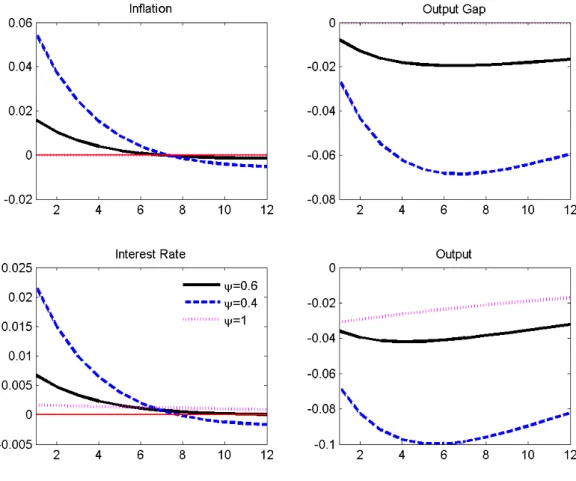
Figure 4.3 shows the optimal unconstrained impulse response functions to an oil price shock of size one for different values of the elasticity of substitution (ψ) for inflation, welfare-relevant output gap, the nominal interest rate and inflation. Inflation and the nominal interest rate are in yearly terms. The benchmark case is a value of ψ = 0.6, similar to the one used by Castillo et.al. (2007). In these graphs we can see that after an oil shock the optimal response
Figure 4.3: Impulse response to an oil shock under optimal monetary policy.
is an increase of inflation and a reduction of the welfare-relevant output gap, and consequently also of output. The nominal interest rate also increases to partially offset the effects of the oil shock on inflation. Inflation after 8 quarters become negative as the optimal unconstrained plan is associated to price stability. To summarise, the optimal response to an oil shock imply an effect on impact on inflation that dies dies out very rapidly and a more persistent effect on output.
A reduction in the elasticity of substitution from 0.6 to 0.4 magnifies the size of the cost push shock, and increases α but reduces λ. Then, the impact on all the variables increases exponentially, being inflation initially the more affected variable. However, after 8 quarters the response is magnified on the welfare relevant output gap. In contrast, when the elasticity of substitution is unity, since there is no such a trade-off, both inflation and welfare-relevant output gap are zero in every period. There is also a reduction on output caused by the oil shock and the increase on the interest rate needed to maintain zero inflation.
4.2 Evaluation of suboptimal rules - the non-inertial plan
We can use our linear-quadratic policy problem for ranking alternative sub-optimal policies. One example of such policies is the optimal non-inertial plan. By a non-inertial policy we mean on in which the monetary policy rule depends only in the current state of the economy. In this case, if the policy results in a determinate equilibrium, then the endogenous variables depend also on the current state.
If the current state of the economy is given by the cost push shock, which has the following law of motion:
ut=ρut−1+$ξt
where ξt is the oil price shock and $ is defined in the previous section. A first order general description of the possible equilibrium dynamics can be written in the form 7:
πt = π+fπut (4.4)
xt = x+fxut (4.5)
ϕt = ϕ+fϕut (4.6)
where we need to determine the coefficients: π, x, ϕ, fπ, fx and fϕ. To solve for the optimal non-inertial plan we need to replace (4.4),(4.5) and (4.6) in the Lagrangian (4.1) and solve for the coefficients that maximise the objective function. The results are summarised in the following proposition:
Proposition 6 The optimal non-inertial plan is given by πt =π+fπut and xt = x+fxut,
where π = 0 fπ = κ2 λ(1−ρ) y+λ(1−βρ)(1−ρ) x= 0 fx = κy κ2 y+λ(1−βρ)(1−ρ)
Note that in the optimal non-inertial plan the ratio of inflation/output gap is constant and equal to λ(1κ−ρ)
y . The higher the weight in the loss function for output fluctuations relative to inflation fluctuations, the higher the inflation rate. Also, the more persistent the oil shocks, the lower the weight on inflation relative to the welfare-relevant output-gap.
Similar the the optimal case, the impulse response functions for inflation and output are defined by:
Itni(πt+j) = fπ$ρjξt
Itni(xt+j) = fπ$ρjξt
Figure 4.4 shows the optimal non-inertial plan to an unitary oil price shock. In this case, the ratio of inflation to the welfare-relevant output gap is constant. For the benchmark case (ψ = 0.6) the response of inflation is lower than in the unconstrained optimal plan, but the
7
Note that in this sub-section we focus on the simplest case of the non-inertial plan, in which all endogenous variables depends only the current state of the economy. In contrast, Benigno and Woodford (2005) work with a different non-inertial plan, in which the lagrange multipliers satisfy the first order conditions of the
effect on output is higher. Also, the effects on both variables are more persistent than in the unconstrained plan.
Furthermore, under the optimal non-inertial plan, when ψ decreases from 0.6 to 0.4 the impact on all the variables increases. This is due to the magnifying effect of ψ on the cost-push shock. Also, the reduction of ψ diminishesλ, which increases more the effect on output relatively to inflation. As in the unconstrained case, whenψ= 1 the trade-off disappears. In that case, inflation is zero in every period and output reduces.
Both exercises, the optimal unconstrained plan and the optimal non-inertial plan, show that to the extent that economies are more dependent on oil, in the sense that oil is difficult to substitute, the impact of oil shocks on both inflation and output is greater. Also, in this case, monetary policy should react by raising more the nominal interest rate and allowing relatively more fluctuations on inflation than on output.
5
Conclusions
This paper characterises the utility-based loss function for a closed economy in which oil is used in the production process, there is staggered price setting and monopolistic competition. As in Benigno and Woodford (2005), our utility based-loss function is a quadratic on inflation and the deviations of output from an efficient level, which is the welfare-relevant output gap.
We found that this efficient level differs from the natural level of output when the elasticity of substitution between labour and oil is different from one. This generates a trade-off between stabilising inflation and output in the presence of oil shocks. Also, the cost-push shocks involved in this trade-off are proportional to oil shocks. The lower this elasticity of substitution, the higher the size of the cost-push shock. We also find, in contrast to Benigno and Woodford (2005), that this trade-off remains even when the effects of monopolistic distortions on the steady state are eliminated.
Furthermore, the relative weight between the welfare-relevant output gap and inflation on the utility-based loss function depends directly to this elasticity of substitution. On the contrary, the higher the share of oil in the production function, the relative weight is smaller. These results show that to the extent that economies are more dependent on oil, in the sense that oil is difficult to substitute in production, the impact of oil shocks on both inflation and output is higher. Also, in this case the central bank should allow less fluctuations on inflation relative to output due to oil shocks.
Moreover, these results shed light on how technological improvements which reduces the dependence on oil, also reduce the impact of oil shocks on the economy. This could also explain why oil shocks have lower impact on inflation in the 2000s in contrast to the 1970s. Since oil has become easier to substitute with other renewable resources, the impact of oil shocks has been dampened. An observation that accords with the theoretical model provided in this paper.
References
[1] Abel, A. (1990), Asset Prices under Habit Formation and Catching up with the Joneses. The American Economic Review, Vol 80 No2 pp38-pp42.
[2] Blanchard, Olivier and Jordi Gali (2005) , Real Wage Rigidities and the New Keynesian Model, mimeo Pompeu Fabra University.
[3] Benigno, Pierpaolo and Michael Woodford (2003), Optimal Monetary Policy and Fiscal Policy,NBER Macroeconomic Annual 2003, Cambridge, MA: MIT Press
[4] Benigno, Pierpaolo and Michael Woodford (2004), Optimal Stabilization Policy when Wages and Prices are sticky: The Case of a Distorted Steady-state, NBER working paper 10839.
[5] Benigno, Pierpaolo and Michael Woodford (2005)” “Inflation Stabilization and Welfare: The Case of a Distorted Steady State”, Journal of the European Economic Association, 3(6): 1-52 .
[6] Calvo, Guillermo (1983), Staggered Prices in a Utility Maximizing Framework. Journal of Monetary Economics, 12, 383-398.
[7] Campbell, and Cochrane J (1999), By Force of Habit: A Consumption-Based Explanation of Aggregate Stock Market Behaviour. The Journal of Political Economy, Vol 107, No 2, 205-251.
[8] Castillo, Paul, Carlos Montoro and Vicente Tuesta (2007), Inflation Premium and Oil Price Volatility. CEP-LSE Discussion Paper N 782.
[9] Clarida, Richard, Jordi Gali, and Mark Gertler (1999), The Science of Monetary Policy: A new Keynesian Perspective.Journal of Economic Literature,pp 1661-1707.
[10] Clarida, Richard, Jordi Gali, and Mark Gertler (2000), Monetary Policy Rules and Macroeconomic Stability: Evidence and Some Theory, Quarterly Journal of Economics,
115, pp. 147-80.
[11] De Paoli, Bianca (2004), Monetary Policy and Welfare in a Small Open Economy, CEP Discussion Paper N◦639 .
[12] Hamilton, James (2003), What is an oil Shock?,Journal of Econometrics, 36, 265-286 [13] Hamilton, James and Ana Herrera (2004), Oil Shocks and Aggregate Macroeconomic
Behavior: The Role of Monetary Policy,Journal of Money Credit and Banking 36, 265-286.
[14] In-Moo Kim and Prakash Loungani (1992), The role of energy in real business cycle models.Journal of Monetary Economics 20, 173-189.
[15] Karotkin, Drora (1996), Justification of the Simple majority and chairman rules, Social Choice and Welfare 13, 479-486.
[16] King, Robert, Charles Plosser and Sergio Rebelo (1988), Production, Growth and Business Cycles, Journal of Monetary Economics 21, 195-232.
[17] Leduc, Sylvian and Keith Sill (2004), A Quantitative Analysis of Oil-price Shocks, Sys-tematic Monetary Policy, and Economic Downturns,Journal of Monetary Economics, 51,
781-808.
[18] Rotemberg, Julio (1982), Sticky prices in the United States, Journal of Political Economy, 90, 1187-1211.
[19] Rotermberg Julio and Woodford Michel (1996), Imperfect Competition and the Effects of Energy Price Increases on Economic Activity,Journal of Money, Credit and Banking.
Vol 28. N◦4.
[20] Rotemberg, Julio and Michael Woodford (1997), An Optimization-based econometric Framework of the Evaluation of Monetary Policy, NBER Macroeconomics Annual, 12:297-346.
[21] Woodford, Michael(1999), Optimal Monetary Policy Inertia, NBER working paper 7261. [22] Woodford, Michael (2003), Interest and Prices: Foundations of a Theory of Monetary
Policy, The Princeton University Press.
[23] Yun, Tack (2005),Optimal Monetary Policy with Relative Price Distortions, The American Economic Review, 95(1), 89-109.
A
Appendix: The deterministic steady state
The non-stochastic steady state of the endogenous variables for Π = 1 is given by:
Interest rate R=β−1 Marginal costs M C = 1/µ Real wages W/P = 1−µα 1−α 1−α 1−1ψ Output Y =1−µα 1 σ+ν 1−α 1−α 1+σ+ψνν 1−1ψ Labor L= 1−α µ σ+1ν 1−α 1−α 1σ−+σψν 1−1ψ
Table A.1: The deterministic steady state
where α=αψ (1 +τq)Q M C 1−ψ =αψ µ(1 +τq)Q1−ψ
α is the share of oil in the marginal costs. Notice that the steady state values of real wages, output and labour depend on the steady state ratio of oil prices with respect to the marginal cost. This implies that permanent changes in oil prices would generate changes in the steady state of this variables. Also, as the standard New-Keynesian models, the marginal cost in steady state is equal to the inverse of the mark-up
M C = µ−1 = (ε−1) (1−τy) ε −1 ≡ 1−Φ
Since monopolistic competition affects the steady state of the model, output in steady state is below the efficient level. We call to this feature a distorted steady state and Φ accounts effects of the monopolistic distortions in steady state.
Since the technology has constant returns to scale, we have that:
VL UC L Y = W/P M C L Y ! M C = (1−α) (1−Φ)
the ratio of the marginal rate of substitution multiplied by the ratio labour/output is a proportion (1−α) of the marginal costs. This expression helps us to obtain the wedge between the marginal rate of substitution between consumption and leisure and the marginal product
of labour: VL UC ∂L ∂Y = VL UC L Y ∂L/L ∂Y /Y ! = (1−α) (1−Φ) (1−δ(σ+v)) ≡ 1−ΦL
where 1−ΦL accounts for the effects of the monopolistic distortions on the wedge between the marginal rate of substitution between consumption and leisure and the marginal product of labour.
B
Appendix: The second order solution of the model
B.1 The recursive AS equation
We divide the equation for the aggregate price level (2.17) byPt1−ε and make Pt/Pt−1= Πt
1 =θ(Πt)−(1−ε)+ (1−θ) Pt∗(z) Pt 1−ε (B-1)
Aggregate inflation is function of the optimal price level of firm z. Also, from equation (2.14) the optimal price of a typical firm can be written as:
Pt∗(z)
Pt
= Nt
Dt
where, after using the definition for the stochastic discount factor: ζt,t+k=βk
C t+k Ct −σ Pt Pt+k, we defineNtand Dtas follows:
Nt = Et "∞ X k=0 µ(θβ)kFt,tε+kYt+kCt−+σkM Ct+k # (B-2) Dt = Et "∞ X k=0 (θβ)kFt,tε−+1kYt+kCt−+σk # (B-3)
Nt and Dt can be expanded as:
Nt = µYtCt−σM Ct+Et " Πεt+1 ∞ X k=0 µ(θβ)k+1Ftε+1,t+1+kYt+1+kCt−+1+σ kM Ct+1+k # (B-4) Dt = YtCt−σ+Et " Πεt+1−1 ∞ X k=0 (θβ)k+1Ftε+1−1,t+1+kCt−+1+σ kYt+1+k # (B-5)
The Phillips curve with oil prices is given by the following three equations: θ(Πt)ε−1 = 1−(1−θ) Pt∗(z) Pt 1−ε (B-6) Nt=µYt1−σM Ct+θβEt(Πt+1)εNt+1 (B-7) Dt=Yt1−σ+θβEt(Πt+1)ε−1Dt+1 (B-8) where we have reordered equation (B-1) and we have used equations (B-2) and (B-3) evaluated one period forward to replace Nt+1 and Dt+1 in equations (B-4) and (B-5).
B.2 The second order approximation of the system
B.2.1 The MC equation and the labour market equilibrium
The real marginal cost (2.12) and the labour market equations (2.4 and 2.23) have the following second order expansion:
mct= (1−α)wt+αqt+ 1 2α(1−α) (1−ψ) (wt−qt) 2 +O kξtk3 (B-9) wt=νlt+σyt (B-10) lt=yt−ψ(wt−mct) +∆bt (B-11)
Wherewtand∆btare, respectively, the log of the deviation of the real wage and the price
disper-sion measure from their respective steady state. Notice that equations (B−10) and (B−11) are not approximations, but exact expressions. Solving equations (B−10) and (B−11) for the equilibrium real wage:
wt= 1 1 +νψ h (ν+σ)yt+νψmct+v∆bt i (B-12)
Plugging the real wage in equation (B−9) and simplifying:
mct = χ(σ+v)yt+ (1−χ) (qt) +χv∆bt (B-13) +1 2 1−ψ 1−αχ 2(1−χ) [(σ+v)y t−qt]2+O kξtk3
whereχ≡(1−α)/(1 +vψα).This is the equation (3−ii) in the main text. This expression is the second order expansion of the real marginal cost as a function of output and the oil prices. Similarly, we can express labour in equilibrium as a function of of output and oil prices:
lt=yt−δ[(v+σ)yt−qt] + χ 1−α∆bt+ 1 2 1−ψ 1−αδχ 2[(v+σ)y t−qt]2+O kξtk3 (B-14) for: δ≡ψχ α 1−α
B.2.2 The price dispersion measure
The price dispersion measure is given by
∆t= Z 1 0 Pt(z) Pt −ε dz
Since a proportion 1−θof intermediate firms set prices optimally, whereas the other θset the price last period, this price dispersion measure can be written as:
∆t= (1−θ) Pt∗(z) Pt −ε +θ Z 1 0 Pt−1(z) Pt −ε dz
Dividing and multiplying by (Pt−1)−ε the last term of the RHS:
∆t= (1−θ) Pt∗(z) Pt −ε +θ Z 1 0 Pt−1(z) Pt−1 −ε Pt−1 Pt −ε dz
SincePt∗(z)/Pt=Nt/DtandPt/Pt−1 = Πt, using equation (2.8) in the text and the definition for the dispersion measure lagged on period, this can be expressed as
∆t= (1−θ)
1−θ(Πt)ε−1 1−θ
!ε/(ε−1)
+θ∆t−1(Πt)ε (B-15)
which is a recursive representation of ∆tas a function of ∆t−1 and Πt.
Benigno and Woodford (2005) show that a second order approximation of the price disper-sion depends solely on second order terms on inflation. Then, the second order approximation of equation (B-15) is: b ∆t=θ∆bt−1+ 1 2ε θ 1−θπ 2 t +O kξtk3 (B-16)
which is equation (3−iii) in the main text. Moreover, we can use equation (B−16) to write the infinite sum:
∞ X t=to βt−to b ∆t = θ ∞ X t=to βt−to b ∆t−1+ 1 2ε θ 1−θ ∞ X t=to βt−toπ 2 t 2 +O kξtk3 (1−βθ) ∞ X t=to βt−to b ∆t = θ∆bto−1+ 1 2ε θ 1−θ ∞ X t=to βt−toπ 2 t 2 +O kξtk3
Dividing by (1−βθ) and using the definition ofκ:
∞ X t=to βt−to b ∆t= θ 1−βθ∆bto−1+ 1 2 ε κ ∞ X t=to βt−toπ 2 t 2 +O kξtk3 (B-17)
The discounted infinite sum of∆btis equal to the sum of two terms, on the initial price dispersion
B.2.3 The second order approximation of the Phillips Curve
The second order expansion for equations (B−6), (B−7) and (B−8) are:
πt= (1−θ) θ (nt−dt)− 1 2 (ε−1) 1−θ (πt) 2+Okξ tk3 (B-18) nt= (1−θβ) at+ 1 2a 2 t +θβ Etbt+1+ 1 2Etb 2 t+1 −1 2n 2 t +O kξtk3 (B-19) dt= (1−θβ) ct+ 1 2c 2 t +θβ Etet+1+ 1 2Ete 2 t+1 −1 2d 2 t +O kξtk3 (B-20)
Where we have defined the auxiliary variables at,bt+1,ctand et+1 as:
at≡(1−σ)yt+mct bt+1 ≡επt+1+nt+1
ct≡(1−σ)yt et+1≡(ε−1)πt+1+dt+1
Subtract equations (B−19) and (B−20), and using the fact thatX2−Y2 = (X−Y) (X+Y), for any two variables X and Y :
nt−dt = (1−θβ) (at−ct) + 1 2(1−θβ) (at−ct) (at+ct) (B-21) +θβEt(bt+1−et+1) + 1 2θβEt(bt+1−et+1) (bt+1+et+1) −1 2(nt−dt) (nt+dt) +O kξtk3
Plugging in the values ofat,bt+1,ctand et+1 into equation (B−21), we obtain: (B−22)
nt−dt = (1−θβ)mct+ 1 2(1−θβ)mct(2 (1−σ)yt+mct) (B-22) +θβEt(πt+1+nt+1−dt+1) +1 2θβEt(πt+1+nt+1−dt+1) ((2ε−1)πt+1+nt+1+dt+1) −1 2(nt−dt) (nt+dt) +O kqt, σqk3
Taking forward one period equation (B−18), we can solve fornt+1−dt+1:
nt+1−dt+1 = θ 1−θπt+1+ 1 2 θ 1−θ (ε−1) 1−θ (πt+1) 2+Okξ tk3 (B-23)
replace equation (B−23) in (B−22) and make use of the auxiliary variablezt= (nt+dt)/(1−θβ)
nt−dt = (1−θβ)mct+ 1 2(1−θβ)mct(2 (1−σ)yt+mct) (B-24) + θ 1−θβ Etπt+1+ ε−1 1−θ +ε Etπt2+1+ (1−θβ)Etπt+1zt+1 −1 2 θ 1−θ(1−θβ)πtzt+O kξtk3
Notice that we use only the linear part of equation (B−23) when we replacent+1−dt+1 in the quadratic terms because we are interested in capture terms only up to second order of accuracy. Similarly, we make use of the linear part of equation (B−18) to replace (nt−dt) = 1−θθπt in the right hand side of equation (B−24). Replace equation (B−24) in (B−18):
πt = κmct+ 1 2κmct(2 (1−σ)yt+mct) (B-25) +β Etπt+1+ ε−1 1−θ +ε Etπt2+1+ (1−θβ)Etπt+1zt+1 −1 2(1−θβ)πtzt− 1 2 (ε−1) 1−θ (πt) 2 +O kξtk3 for κ≡ (1−θ) θ (1−θβ)
wherezt has the following linear expansion:
zt= 2 (1−σ)yt+mct+θβEt 2ε−1 1−θβπt+1+zt+1 +O kξtk3 (B-26)
Define the following auxiliary variable:
vt=πt+ 1 2 ε−1 1−θ +ε πt2+1 2(1−θβ)πtzt (B-27) Using the definition for vt, equation (B−25) can be expressed as:
vt=κmct+ 1 2κmct(2 (1−σ)yt+mct) + 1 2επ 2 t +βEtvt+1+O kξtk3 (B-28)
which is equation (3−iv) in the main text.
Moreover, the linear part of equation (B-28) is:
πt=κmct+βEt(πt+1) +O
kξtk3
which is the standard New Keynesian Phillips curve, inflation depends linearly on the real marginal costs and expected inflation.
Replace the equation for the marginal costs (B-13) in the second order expansion of the Phillips curve (B-28) vt = κyyt+κqqt+κχv∆bt+ 1 2επ 2 t + (B-29) +1 2κ cyyyt2+ 2cyqytqt+cqqq2t +βEtvt+1+O kξtk3
where the coefficients coefficients of the linear part are given by
κy = κχ(σ+ν)
and those of the quadratic part are: cyy = χ(σ+ν) [2 (1−σ) +χ(σ+ν)] + (1−ψ) χ2(1−χ) (σ+ν)2 1−α cyq = (1−χ) [2 (1−σ) +χ(σ+ν)]−(1−ψ) χ2(1−χ) (σ+ν) 1−α cqq = (1−χ)2+ (1−ψ) χ2(1−χ) 1−α
Equation B-29 is a recursive second order representation of the Phillips curve. However, we need to express the price dispersion in terms of inflation in order to have a the Phillips curve only as a function of output, inflation and the oil shock. Equation B-29 can also be expressed as the discounted infinite sum:
vto = ∞ X t=to βt−to κyyt+κqqt+κχv∆bt+ 1 2επ 2 t + 1 2κ cyyyt2+ 2cyqytqt+cqqqt2 +kξtk3
after making use of equation B-17, the discounted infinite sum of ∆bt,vto becomes
vto = ∞ X t=to βt−to κyyt+κqqt+ 1 2ε(1 +χv)π 2 t + 1 2κ cyyyt2+ 2cyqytqt+cqqqt2 + χvθ 1−βθ∆bto−1+ kξtk3 (B-30) which is equation (3.2) in the main text.
B.3 A second-order approximation to utility
The expected discounted value of the utility of the representative household
Uto =Eto ∞ X t=to βt−to[u(C t)−v(Lt)] (B-31)
The first term can be approximated as:
u(Ct) =Cuc ct+ 1 2(1−σ)c 2 t +t.i.p.+Okξtk3 (B-32)
Similarly, the second term:
v(Lt) =LvL lt+ 1 2(1 +ν)l 2 t +t.i.p.+O kξtk3 (B-33)
Replace the equation for labour in equilibrium in B-33:
v(Lt) =LvL vyyt+ 1 2vyyy 2 t +vyqytqt+v∆∆bt +t.i.p.+O kξtk3 (B-34)
where: vy = 1−δ(v+σ) vyy = (1 +v) (1−δ(v+σ))2+ 1 2 1−ψ 1−αχ 2δ(σ+v)2 vyq = (1 +v)δ(1−δ(v+σ))− 1 2 1−ψ 1−αχ 2δ2(σ+v) v∆ = χ 1−α
We make use on the following relation:
LvL= (1−Φ) (1−α)Y uc (B-35) where Φ = 1− 1
µ = 1− 1−τ
ε/(ε−1) is the steady state distortion from monopolistic competition. Replace the previous relation, equation B-32 and B-34 in B-31, and make use of the clearing market condition: Ct=Yt Uto =Y uc ∞ X t=to βt−to uyyt+ 1 2uyyy 2 t +uyqytqt+u∆∆bt +t.i.p.+Okξtk3 (B-36) where uy = 1−(1−Φ) (1−α)vy = ΦL uyy = 1−σ−(1−Φ) (1−α)vyy = 1−σ−(1−ΦL)vyy/(1−δ(v+σ)) uyq = −(1−Φ) (1−α)vyq =−(1−ΦL)vyq/(1−δ(v+σ)) u∆ = −(1−Φ) (1−α)v∆=−(1−Φ)χ where we make use of the following change of variable:
ΦL= 1−(1−Φ) (1−α) (1−δ(v+σ)) (B-37) where ΦLis the effective effect of the monopolistic distortion in welfare through the of output. Notice that when we eliminate the monopolistic distortion, i.e. Φ = 0, ΦL is not necessarily equal to zero.
Replace the present discounted value of the price distortion (B-17) in B-36:
Uto =Y ucEto ∞ X t=to βt−to uyyt+ 1 2uyyy 2 t +uyqytqt+ 1 2uππ 2 t +t.i.p.+Okqtk3 (B-38) where uπ = ε κu∆=−(1−Φ)χ ε κ
Use equation B-30, the second order approximation of the Phillips curve, to solve for the expected level of output:
∞ X t=to βt−toy t = − 1 κy ∞ X t=to βt−to κqqt+ 1 2ε(1 +χv)π 2 t + 1 2κ cyyyt2+ 2cyqytqt+cqqq2t + 1 vt −χv(1−θ)∆bt−1 +kξtk3 (B-39)
Replace equation B-39 in B-38 to express it as function of only second order terms: Uto =−ΩEto ∞ X t=to βt−to 1 2λy(yt−y ∗ t)2+ 1 2λππ 2 t +Tto +t.i.p.+O kqtk3 (B-40)
which is equation B-35 in the text, where:
λy = ΦL κ κy cyy−uyy λπ = ΦL ε(1 +χv) κy −uπ yt∗ = −ΦL κ κycyq−uyq ΦLκκycyy−uyy qt
additionally we have thatΩ =Y uc and Tto =Y uc ΦL
κyvto Make use of the following auxiliary variables:
ω1 = (1−σ) ΦL+χ(σ+v) ω2 = χ(σ+v) 1−χ 1−α + (1−ΦL) σψα 1−σψα ω3 = ΦLσα
then, λy,λπ and yt∗ can be written as a function ofω1,ω2 and ω3
λy = ω1+ (1−ψ)ω2 λπ = ε κy(1−σψα) [ω1+ (1−ψ)ω3] y∗t = − 1−χ χ(σ+v) " ω1−(1−ψ)1−χχω2 ω1+ (1−ψ)ω2 # qt using the definitions forχ,yt∗ can be expressed as:
y∗t =− 1 +ψv σ+v α 1−α+η (B-41) where η≡ (1−ψ) (1−α)ω2 (1−χ)ω1−(1−ψ)χω2
Denoteα∗, the efficient share in steady state of oil in the marginal costs, where
α∗ = α 1 +η thenyt∗ is y∗t =− 1 +ψv σ+v α∗ 1−α∗ qt (B-42)
Note from the definition for η that whenψ = 1, then η = 0, α∗ =α =α and yt∗ =ynt. For a Cobb-Douglas production function the efficient level of output equals the natural level. Also, when ψ <1, then η >0, α∗ < αand |y∗t|<|ynt|. For elasticity of substitution between inputs lower than one the efficient level fluctuates less to oil shocks than the natural level. Also note that even when ΦLis equal to zero, which summarises the effect of monopolistic distortions on the wedge between the marginal rate of substitution and the marginal product of labour,η is still different than zero forψ6= 1.This indicates that the efficient level of output still diverges from the natural level even we eliminate the effects of monopolistic distortions.
In the same way, the natural rate of output can be expressed as:
ynt =− 1 +ψv σ+v α 1−α qt (B-43)
Similarly, we can simplify λ=λy/λπ as:
λ= λy
λπ
= κy(1−σψα)
ε γ
where we use the auxiliary variable:
γ ≡
ω1+ (1−ψ)ω2
ω1+ (1−ψ)ω3
Note that when ψ= 1, thenγ = 1 and when ψ <1, thenγ = 1 sinceω2 > ω3.
C
Appendix: Optimal Monetary Policy
C.1 Optimal response to oil shocks
The policy problem consists in choosingxtand πtto maximise the following Lagrangian:
L=−Eto ( ∞ X t=to βt−to 1 2λx 2 t + 1 2π 2 t −ϕt(πt−κyybt−βEtπt+1−ut) +ϕto−1 πto−π ∗ to ) whereβt−toϕ
t is the Lagrange multiplier associated with the constraint at time t The first order conditions with respect to πtand yt are respectively
πt = ϕt−1−ϕt (C-1)
λxt = κyϕt (C-2)
and for the initial condition:
πto =π ∗
to
where π∗to is the initial value of inflation which is consistent with the policy problem in a ”timeless perspective”.
Replace conditions C-1 and C-2 in the Phillips Curve:
βEtϕt+1−
(1 +β)λ+κ2yϕt+λϕt−1=λut (C-3) this difference equation has the following solution8 :
ϕt=τϕϕt−1−τϕ
X∞
j=0β jτj
ϕEtut+j (C-4) whereτϕ is the characteristic root, lower than one, of C-3, and it is equal to
τϕ =Z− r Z2− 1 β forZ =(1 +β) +κ 2 y λ
/(2β).Since the oil price follows an AR(1) process of the form:
qt=ρqt−1+ξt
and the mark-up shock is: ut=$qt, thenutfollows the following process:
ut=ρut−1+$ξt (C-5)
Solution to the optimal problemTaking into account C-5, equation C-4 can be expressed as: ϕt=τϕϕt−1−φqt (C-6) where: φ= τϕ 1−βτϕρ $
Initial conditionIterate backward equation (C-6) and evaluate it atto−1, this is the timeless solution to the initial conditionϕto−1:
ϕto−1 =−φΣ ∞
k=0(τϕ)kqto−1−k (C-7) which is a weighted sum of all the past realisations of oil prices.
Equations (C-1), (C-2), (C-6) and (C-7) are the conditions for the optimal unconstrained plan presented in proposition 3.5. Impulse responsesAn innovation ofξtto the real oil price affects the current level and the expected future path of the lagrange multiplier by an amount:
Etϕt+j −Et−1ϕt+j =−
ρj+1−(τ ϕ)j+1
ρ−τϕ
φξt
for eachj ≥0.Given this impulse response for the multiplier. (C-1) and (C-2) can be used to derive the corresponding impulse responses for inflation and output gap:
Etπt+j −Et−1πt+j = " ρj+1−(τϕ)j+1 ρ−τϕ − ρ j−(τ ϕ)j ρ−τϕ # φξt Etyt+j−Et−1yt+j = − κy λ ρj+1−(τϕ)j+1 ρ−τϕ φξt which are expressions that appear in the main text.
C.2 The optimal Non-inertial plan
We want to find a solution for the paths of inflation and output gap such that the behaviour of endogenous variables is function only on the current state. That is:
πt = π+fπut (C-8)
xt = x+fxut (C-9)
ϕt = ϕ+fϕut (C-10)
where the coefficientsπ, y, ϕ, fπ, fx and fϕ are to be determined
Replace (C-8), (C-9) and (C-10) in the Lagrangian and take unconditional expected value:
−E(Lto) ≡ E Eto ∞ X t=to βt−to 1 2λ(x+fxut) 2+1 2(π+fπut) 2 −(ϕ+fϕut) (1−β)π−κyx + (1−βρ)fπut−ut−κyfxut +E((ϕ+fϕuto−1) [π+fπuto]) (C-11)
suppressing the terms that are independent of policy and using the law of motion forut, this can be simplified as:
−E(Lto) ≡ 1 2 (1−β) λx 2+π2 − 1 2 (1−β)ϕ((1−β)π−κyx) +1 2 σ2u 1−β λfx 2+f π2 −1 2 σu2 1−βfϕ((1−βρ)fπ−1−κyfx) +ρσu2fϕfπ
the problem becomes to findπ, y, ϕ, fπ, fx andfϕ such that maximise the previous expression. Those coefficients are:
π = x=ϕ= 0 fπ = λ(1−ρ) λ(1−βρ) (1−ρ) +κ2 y fx = − κy λ(1−βρ) (1−ρ) +κ2 y fϕ = λ λ(1−βρ) (1−ρ) +κ2 y
Documentos de Trabajo publicados
Working Papers published
La serie de Documentos de Trabajo puede obtenerse de manera gratuita en formato pdf en la siguiente dirección electrónica:
http://www.bcrp.gob.pe/bcr/Documentos-de-Trabajo/Documentos-de-Trabajo.html
The Working Paper series can be downloaded free of charge in pdf format from:
http://www.bcrp.gob.pe/bcr/ingles/working-papers/working-papers.html
2007
Mayo \ May
DT N° 2007-009
Estimación de la Frontera Eficiente para las AFP en el Perú y el Impacto de los Límites de Inversión: 1995 - 2004
Javier Pereda DT N° 2007-008
Efficiency of the Monetary Policy and Stability of Central Bank Preferences. Empirical Evidence for Peru
Gabriel Rodríguez DT N° 2007-007
Application of Three Alternative Approaches to Identify Business Cycles in Peru Gabriel Rodríguez
Abril \ April
DT N° 2007-006
Monetary Policy in a Dual Currency Environment Guillermo Felices, Vicente Tuesta
Marzo \ March
DT N° 2007-005
Monetary Policy, Regime Shift and Inflation Uncertainty in Peru (1949-2006) Paul Castillo, Alberto Humala, Vicente Tuesta
DT N° 2007-004
Dollarization Persistence and Individual Heterogeneity Paul Castillo y Diego Winkelried
DT N° 2007-003
Why Central Banks Smooth Interest Rates? A Political Economy Explanation Carlos Montoro
Febrero \ February
DT N° 2007-002
Comercio y crecimiento: Una revisión de la hipótesis “Aprendizaje por las Exportaciones”
Raymundo Chirinos Cabrejos
Enero \ January
DT N° 2007-001
Perú: Grado de inversión, un reto de corto plazo Gladys Choy Chong
2006
Octubre \ October
DT N° 2006-010
Dolarización financiera, el enfoque de portafolio y expectativas: Evidencia para América Latina (1995-2005)
Alan Sánchez DT N° 2006-009
Pass–through del tipo de cambio y política monetaria: Evidencia empírica de los países de la OECD
César Carrera, Mahir Binici
Agosto \ August
DT N° 2006-008
Efectos no lineales de choques de política monetaria y de tipo de cambio real en economías parcialmente dolarizadas: un análisis empírico para el Perú
Saki Bigio, Jorge Salas
Junio \ June
DT N° 2006-007
Corrupción e Indicadores de Desarrollo: Una Revisión Empírica Saki Bigio, Nelson Ramírez-Rondán
DT N° 2006-006
Tipo de Cambio Real de Equilibrio en el Perú: modelos BEER y construcción de bandas de confianza
Jesús Ferreyra y Jorge Salas DT N° 2006-005
Hechos Estilizados de la Economía Peruana Paul Castillo, Carlos Montoro y Vicente Tuesta DT N° 2006-004