Imagem
Diogo Júdice
Trust-Region Methods
without using Derivatives:
Worst-Case Complexity
and the Non-Smooth Case
Tese de Doutoramento do Programa Inter-Universitário de Doutoramento
em Matemática, orientada pelo Professor Doutor Luís Nunes Vicente e
apresentada ao Departamento de Matemática da Faculdade de Ciências e
Tecnologia da Universidade de Coimbra.
Trust-Region Methods
without using Derivatives:
Worst Case Complexity
and the Non-Smooth Case
Diogo Júdice
UC|UP Joint PhD Program in Mathematics
Programa Inter-Universitário de Doutoramento em Matemática
PhD Thesis | Tese de Doutoramento
Acknowledgements
I would like to express my deepest and sincere gratitude to Professor Luís Nunes Vicente. Since the beginning of this journey, he has always pointed me in the right direction, both scientifically and personally. It would have been impossible to fulfill this task without him. I believe that I am now a better mathematician and a better person, mostly because of his guidance.
I would like to thank Dr. R. (Nima) Garmanjani for his help regarding the numerical experiments and his revision of this dissertation. I would also like to thank also Mrs Rute Andrade for having helped me in so many administrative matters.
I am grateful to Fundação para a Ciência e Tecnologia for having given me financial support (scholarship SFRH/BD/74401/2010) for my doctoral studies. I would also like to thank the University of Coimbra and, in particular, the Department of Mathematics, for all the academic, administrative, and technical support.
I would like to thank my parents and my siblings for everything. Without them, it would have been impossible to accomplish this task. In particular, I would like to thank my parents for all their help and support during this process. I also would like to thank my friends Miguel Côrte-Real and Benedita Garrett for their support and encouragement in difficult times.
Finally, I would like to dedicate this thesis to my daughters Maria and Matilde and to my brother Pedro.
Abstract
Trust-region methods are a broad class of methods for continuous optimization that found application in a variety of problems and contexts. In particular, they have been studied and applied for problems without using derivatives.
The analysis of trust-region derivative-free methods has focused on global convergence, and they have been proved to generate a sequence of iterates converging to stationarity independently of the starting point. Most of such an analysis is carried out in the smooth case, and, moreover, little is known about the complexity or global rate of these methods. In this thesis, we start by analyzing the worst case complexity of trust-region derivative-free methods for smooth functions (based on a modification of the existent general methodology), bounding the number of iterations and function evaluations to reach a certain threshold of first or second order stationarity.
For the non-smooth case, we propose a smoothing approach, for which we prove global conver-gence and bound the worst case complexity effort. For the special case of non-smooth functions that result of the composition of smooth and non-smooth/convex components, we show how to improve the existing results of the literature using the general modified methodology of the smooth case.
Resumo
Os métodos de região de confiança formam uma classe geral de métodos para optimização contínua que encontram aplicação numa variedade de problemas e contextos. Em particular, estes métodos têm sido estudados e aplicados a problemas sem recurso a derivadas.
A análise dos métodos de região de confiança sem derivadas tem incidido em convergência global, mostrando que estes métodos geram sequências de pontos convergindo para pontos estacionários, independentemente do ponto inicial. Uma grande parte desta análise é feita no caso suave, sabendo-se pouco sobre a complexidade ou taxa global destes métodos. Nesta tese, começamos por analisar a complexidade no pior dos casos de métodos de região de confiança sem derivadas para funções suaves (recorrendo a uma modificação da metodologia geral existente), limitando o número de iterações e de avaliações de função necessárias para atingir uma determinada proximidade a estacionaridade de primeira ou segunda ordem.
Para o caso não suave, propomos uma abordagem de suavização, para a qual provamos convergên-cia global e limitamos a complexidade no pior dos casos. Para o caso especonvergên-cial de funções não suaves resultantes da composição de funções suaves com funções não suaves e convexas, mostramos como melhorar os resultados existentes na literatura utilizando a metodologia geral modificada do caso suave.
Table of contents
List of figures xi
List of tables xiii
1 Introduction 1
1.1 Trust-region methods for DFO . . . 1
1.2 Worst case complexity in DFO . . . 2
1.3 The contribution of this thesis . . . 2
1.4 Organization of the thesis and some terminology . . . 3
2 Derivative-free trust-region methods for smooth functions 5 2.1 Introduction to trust-region methods for smooth functions . . . 5
2.2 Introduction to derivative-free trust-region concepts . . . 11
2.3 A derivative-free trust-region framework for smooth functions . . . 20
2.4 Other derivative-free model-based approaches . . . 27
3 Worst case complexity of algorithms for continuous nonlinear optimization 31 3.1 WCC for optimization with derivatives . . . 31
3.2 WCC for optimization without derivatives . . . 34
4 Worst case complexity of derivative-free trust-region methods 39 4.1 Complexity in determining first-order stationary points . . . 39
4.2 Complexity in determining second-order stationary points . . . 48
5 Derivative-free trust-region methods for non-smooth functions 55 5.1 A review of basic concepts in non-smooth analysis . . . 55
5.2 Smoothing of non-smooth functions . . . 57
5.3 Smoothing trust-region methods without derivatives . . . 60
5.4 Derivative-free trust-region methods for composite functions . . . 64
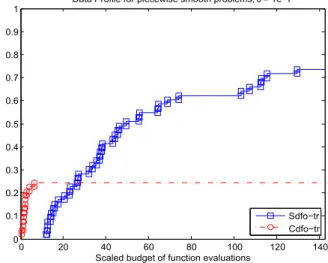
5.5 A numerical illustration . . . 71
6 Conclusion 75
List of figures
5.1 Data profiles computed for a set of piecewise smooth problems, comparing the smoothing and composite trust-region methods. . . 72 5.2 Performance profiles computed for a set of piecewise smooth problems, in a
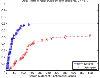
logarith-mic scale, comparing the smoothing and composite trust-region methods. . . 73 5.3 Data profiles computed for a set of piecewise smooth problems, comparing the
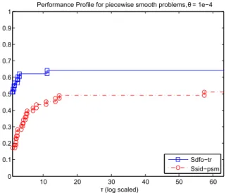
smoothing trust-region and direct-search methods. . . 73 5.4 Performance profiles computed for a set of piecewise smooth problems, in a
logarith-mic scale, comparing the smoothing trust-region and direct-search methods. . . 74
List of tables
Chapter 1
Introduction
1.1
Trust-region methods for DFO
Trust-region methods are iterative methods for the optimization of a function in a continuous space, possibly subject to constraints. In these methods, to obtain a trial point, one typically considers the minimization of a quadratic model in a region around the current iterate and measured by a certain radius. The model serves as a local approximation of the function, in particular of its curvature (see the extensive monograph by Conn, Gould, and Toint [18] and the recent survey paper by Yuan [69]). This thesis concerns trust-region methods for unconstrained derivative-free optimization (DFO), where it is assumed that there is only access to the function values. Derivatives, if they exist, are unavailable or little reliable to be used. DFO problems are common in Engineering Optimization where the evaluation of the functions may be the output of a numerical simulation. DFO has also been relatively well studied (see the book by Conn, Scheinberg, and Vicente [23]). In DFO trust-region methods, the models are frequently built by fitting a sample set using interpolation or regression, and their quality is measured by the accuracy they provide relatively to a Taylor expansion. In particular, fully linear models [20] are those as smooth and accurate as first-order Taylor ones.
Accepting the trial point as the new iterate and updating the trust-region radius depend on how much the function was reduced relatively to the model. If the current iterate is non-stationary and the model has good quality, the algorithms succeed in accepting a trial point as a new iterate in a finite number of reductions of the trust-region radius. These methods have been shown to be convergent to first-order stationary points by Conn, Scheinberg, Toint, and Vicente (in the papers [19, 22]) under the condition that fully linear models are available when necessary. The strict need of controlling geometry or considering model-improvement steps was questioned in [32], where good numerical results were reported for an interpolation-based trust-region method which ignores the geometry of the sample sets. Scheinberg and Toint [63] gave an example showing that geometry cannot be totally ignored and that some form of model improvement is necessary, at least when the size of the model gradient becomes small (a procedure known as the ‘criticality step’, which then ensures that the trust-region radius converges to zero).
1.2
Worst case complexity in DFO
For a long while, DFO methods have been analyzed by establishing their global convergence properties, meaning their asymptotic convergence to stationary regardless of the starting point (see [23, 46]). More recently, there has been some interest in establishing their global rates of convergence or, similarly, bounds on the number of iterations (and of function evaluations) required in the worst case to achieve a certain threshold of stationarity. Such results are derived independently of the starting point which justifies saying that the rates are global.
In part, such a recent effort follows a similar trend occurred for the unconstrained, derivative-based optimization of smooth functions (where the gradient exists and is Lipschitz continuous). Nesterov [52] started by showing that the gradient or steepest descent method takes a number of iterations of the order ofε−2— and we write that asO(ε−2)— to drive the norm of the gradient
of the objective function belowε. This effort is reduced toO(ε−1)in the presence of convexity. It
is known that such a bound is sharp or tight (see the example of Cartis, Gould, and Toint [11]). A similar worst case complexity bound ofO(ε−2)has been proved by Gratton, Sartenaer, and Toint [41] for trust-region methods. The worst case complexity (WCC) bound on the number of iterations can be reduced toO(ε−1.5)for cubic overestimation methods (see Nesterov and Polyak [54] and Cartis, Gould, and Toint [10]).
In the context of DFO, most of the WCC analysis has been carried out for direct-search methods of directional type based on a sufficient decrease condition. The first worst-case complexity bound, ofO(ε−2), was derived by Vicente [64] for smooth functions, and later refined toO(ε−1)when the function is convex by Dodangeh and Vicente [28]. Garmanjani and Vicente [34], using a smoothing approach, have shown a WCC bound ofO(|logε|ε−3)in the non-smooth case. Similar WCC bounds
were derived, in expectation, by Nesterov [53] for his random Gaussian smoothing approach. Cartis, Gould, and Toint [14] have derived a WCC bound ofO(ε−1.5)for their derivative-free adaptive cubic overestimation algorithm, but using finite differences to approximate derivatives.
1.3
The contribution of this thesis
In this thesis we address the worst case complexity of trust-region methods for unconstrained DFO. Our contributions are fourfold.
First we consider the smooth case and, as expected, derive a WCC bound of O(ε−2) for the number of iterations andO(n2ε−2)for the number of function evaluations. There were a number
of delicate issues to overcome, one of which being how to appropriately measure the effort of the criticality step to avoid worsening the powerε−2. It is also nontrivial to appropriately count the number of iterations that are acceptable (the function is decreased, the trial point is accepted as the new iterate, and the radius is reduced) or of model-improvement type (the iterate and the radius are maintained), under the general setting in [22].
A second contribution is again in the smooth case but related to the WCC of derivative-free trust-region methods when determining second-order critical points. It is known that such methods globally converge to points satisfying the second-order necessary conditions [22]. It is also known that derivative-based trust-region methods require a number of theO(max{εg−2εH−1,ε
−3
1.4 Organization of the thesis and some terminology 3
to determine a point where the norm of the gradient of the objective function is belowεgand the
smallest eigenvalue of the Hessian of the function is above−εH(see Cartis, Gould, and Toint [13]). In
this thesis, we prove a bound ofO(ε−3), withε=εg=εH, when no derivatives are used, and refine it
asO(n5ε−3)under certain assumptions for the corresponding number of functions evaluations. Very
recently, it was proposed in [39] a direct-search method (that may use eigenvectors of approximated Hessians as directions), achieving the same WCC bounds in iterations and function evaluations.
Thirdly, we address the general non-smooth case, and develop a smoothing trust-region approach in the same vein as for direct search [34]. The number of iterations required to drive the smoothing parameter and the norm of the smoothing gradient belowε will be shown to be ofO(|logε|ε−3)(for
function evaluations,O(n2|logε|ε−3)). The knowledge of the contribution [34] has provided some
guidance on how to obtain this result, but a lot had still to be done, from building all necessary blocks from the smooth case to assembling all components in the new context of trust regions.
The fourth contribution addresses the analysis of WCC of derivative-free trust-region methods for composite functions of the typeh(F)wherehis real, non-smooth, and convex andF is vectorial and smooth (but for which derivatives are unavailable). This task was already attempted by Grapiglia, Yuan, and Yuan [37] but under a restrictive setting (relatively to the general scenario in [22]) and with sub-optimal results. Their complexity result in terms of function evaluations is of the form
O(|logε|ε−2), where ours will be justO(ε−2). We were able to remove the factor|logε|precisely
from the way we count iterations in the criticality step. Further, contrary to [37], we do not impose a reduction of the trust-region radius on model-improvement iterations. In terms of function evaluations, our bound looks likeO(ℓn2ε−2), whereℓis the number of functions components inF.
The author of this thesis is a co-author of the paper [33], under review in the SIAM Journal on Optimization, where the first, third, and fourth contributions of this thesis are reported.
1.4
Organization of the thesis and some terminology
This thesis is organized as follows. We start by reviewing trust-region methods with and without derivatives in Chapter 2, focusing on their global convergence properties. Then we review global rates for nonlinear optimization, with and without derivatives, in Chapter 3. Our first two contributions are described in Chapter 4: Section 4.1 for the WCC of derivative-free trust-region methods for determining first-order critical points of smooth functions; Section 4.2 likewise but for second-order critical points. Chapter 5 addresses the non-smooth case. In Section 5.3 we introduce and analyze the smoothing approach. The non-smooth composite case is handled in Section 5.4. At the end of this chapter (Section 5.5), we provide a numerical illustration of the latter two approaches for the case∥F∥1. The thesis is ended in Chapter 6, with some conclusions and prospects of future work.
In the thesis we will refer often to rates of convergence, most of the times in a global sense (where, as opposed to a local sense, no assumption is made on the proximity of the starting point to stationarity). Let{xk}k≥0be a sequence inRnconverging tox∗. Consider the corresponding real sequence defined
byrk=∥xk−x∗∥. We say that{xk}k≥0has a linear rate of convergence if there existsθ∈(0,1)such
thatrk+1/rk≤θfor allksufficiently large. For example, the sequence{(1/2)k}k≥0converges linearly.
The rate of convergence can be slower or faster than linear. For the former case, the sequence{xk}k≥0
zero). Examples of real sequences exhibiting sublinear rates tox∗=0 that appear often in first-order methods for continuous optimization are{1/k2}k≥0,{1/k}k≥0, and{1/
√
k}k≥0. For the latter case,
the sequence{xk}k≥0converges superlinearly if the ratiork+1/rk converges to 0 (an example being {(1/2)k2}k≥0 withx∗=0). Finally, we say that the sequence {xk}k≥0 converges quadratically if
rk+1/rk2≤M, for some M>0. An example is given by the sequence{10
−2k}
k≥0 that converges
quadratically tox∗=0. The rates described so far are the q-rates where the “q” stands for quotient, see [56, Chapter 9]. There are also the so-called r-rates (r of root). A sequence converges with an r-rate tox∗ifrk is bounded by a real sequence converging with a q-rate to 0. For instance, the rate of
convergence of the sequence{xk}k≥0is r-linear ifrk≤yk and{yk}k≥0converges linearly to 0∈R.
An example is given by the sequence defined byxk= (1/2)k fork even andxk=0 fork odd. In
both cases, q and r, what we have described are consequences of the original, more complicated definitions [56, Chapter 9].
In the WCC bounds, the notation O(A)will mean a scalar timesA, where the scalar does not depend on the iteration counter of the method under analysis (thus depending only on the problem or on algorithmic constants). The dependence ofAon the dimensionnof the problem (or on a Lipschitz constant) will be made explicit whenever appropriate.
The notationB(x;∆)stands for{y∈Rn:∥y−x∥ ≤
∆}and by default all norms are the Euclidean ones.
Chapter 2
Derivative-free trust-region methods for
smooth functions
In this chapter we will review the basic concepts of trust-region algorithms for the unconstrained minimization of a smooth function f:Rn→R, with or without derivatives.
Section 2.1 is devoted to the basics of trust-region methods in the presence of derivatives. We use a simple trust-region method to describe the concepts involved, in particular the quadratic models and the trust-region subproblem. The algorithm described converges to first and second order stationary points. We will also comment on the local rate convergence of a Newton’s method globalized by such trust-region scheme. This material is now classic and a more comprehensive coverage is given in the book by Conn, Gould, and Toint [18], in [55, Chapter 4], and in the survey papers [48, 69]. The proofs of the results stated in this section can be found in [18].
In Section 2.2 we start to address trust-region methods but without the use of derivatives. The necessary tools for global convergence of derivative-free trust-region algorithms are presented. We will show how interpolation and regression techniques can be used to build models with the desired properties. Such models will replace the quadratic models using derivatives defined in Section 2.1. The material is mostly taken from [23].
In Section 2.3 it is presented the derivative-free trust-region framework of [22] (see also [23, Chapter 10]). This framework includes a number of provisions for the absence of derivatives including, for instance, criticality and model-improvement steps. The global convergence properties will be stated and discussed.
In Section 2.4 other derivative-free trust-region approaches are referred and commented.
2.1
Introduction to trust-region methods for smooth functions
A typical trust-region method approximates the objective function by a quadratic model in a neigh-borhood or ball of the current iterate point. Then it minimizes the model in that neighneigh-borhood (trust region). If the model solution is a good approximation for the function f, then the step is taken and the radius of the ball (trust-region radius) is possibly increased. If not, the trust-region radius is shrunk and the model is minimized again. This process is repeated until some form of approximate stationarity is reached.
To be more specific, letxkbe the current iterate. A trust region is typically a set of the form
B(xk;∆k) ={x∈Rn:∥x−xk∥ ≤∆k},
where∆kis the trust-region radius. Assuming that f is continuously differentiable, one can
approxi-mate f inB(xk;∆k)by a quadratic of the form:
mk(xk+s) = fk+g⊤ks+
1 2s
⊤
Hks, (2.1)
where fk = f(xk), gk=∇f(xk)∈Rn, and Hk ∈Rn×n is a symmetric matrix. Observe that from
Taylor’s Theorem, we know that the difference betweenmk(xk+s)and f(xk+s)isO(∥s∥2), which is
small for smalls. When the function is twice continuously differentiable, the matrixHkis seen as
an approximation to the Hessian matrix∇2f(xk). IfHk=∇2f(xk), the difference betweenmk(xk+s)
and f(xk+s)becomesO(∥s∥3). To obtain the next iterate we must findsas an approximate solution
of the trust-region subproblem
min s∈Rn mk(xk+s) = fk+g ⊤ ks+ 1 2s ⊤ Hks s.t. ∥s∥ ≤∆k.
Observe that if Hk is positive definite and ∥Hk−1gk∥ ≤∆k, the exact solution of this problem is
sHk =−Hk−1gk.
The minimizer of the modelmk(xk+s)subject to∥s∥ ≤∆kalong the steepest descent direction −gk=−∇f(xk)is called the Cauchy stepsCk. For the trust-region method to globally converge to
first-order stationarity, the approximate solutionskmust give a decrease onmk(xk+·)as good as the
Cauchy step. It can be shown that [55, Lemma 4.3] mk(xk)−mk(xk+sCk) ≥ 1 2∥gk∥min ∥gk∥ ∥Hk∥ ,∆k ,
where we assume that ∥gk∥
∥Hk∥ = +∞whenHk=0. In fact, to guarantee global convergence to first-order
stationary points we only need the stepskto be as good as the Cauchy step in the sense of
mk(xk)−mk(xk+sk) ≥ κf cd(mk(xk)−mk(xk+sCk)), (2.2)
for some constantκf cd ∈(0,1). Thus, the stepskwill satisfy
mk(xk)−mk(xk+sk) ≥ κf cd 2 ∥gk∥min ∥gk∥ ∥Hk∥ ,∆k . (2.3)
The next step of the trust-region iteration is to measure the quality of the trial stepsk. For this
matter, we compare the decrease in the modelmk, given bymk(xk)−mk(xk+sk), with the actual
decrease in the function f, given by f(xk)−f(xk+sk). We then define the ratio
ρk=
f(xk)−f(xk+sk)
mk(xk)−mk(xk+sk)
2.1 Introduction to trust-region methods for smooth functions 7
The numerator inρk is called theactual reductionand the denominator thepredicted reduction. The
value ofρkis used to accept or not the trial point given byxk+1=xk+sk. First, observe from (2.2)
thatmk(xk)−mk(xk+sk)≥0. So, ifρk<0 the function f increases at the trial point and so it must be
rejected and the trust-region radius decreased (and for the moment we consider that the same is done whenρk∈[0,η)for smallη∈(0,1)). On the other hand, ifρkis bigger thanη∈(0,1), it means that
the model represents the function well in that trust region. In such a case, one accepts the trial step and possibly increase the trust-region radius. A trust-region method is thus an iterative method that starts with an initial guess and an initial trust-region radius. To proceed let us define it now formally.
Algorithm 2.1.1 Trust-region method (for smooth functions; first-order)
Initialization: Choose an initial pointx0 and an initial trust-region radius∆0∈(0,∆max]for some
∆max>0. Construct the initial modelm0(x0+s)as in (2.1). The constantsη∈(0,1),γinc>1,
andγ∈(0,1)are given. Setk=0.
Step 1 (step calculation): Compute a stepsk that sufficiently reduces the modelmk, in the sense
of (2.2).
Step 2 (acceptance of the trial point): Compute f(xk+sk)andρk.
Ifρk≥η, thenxk+1=xk+skand the model of the form (2.1) is constructed at the new iterate
xk+1 resulting in a new modelmk+1(xk+1+s). Otherwise the model and the iterate remain
unchanged (mk+1=mkandxk+1=xk).
Step 3 (trust-region radius update): Set
∆k+1∈
(
[∆k,min{γinc∆k,∆max}] if ρk≥η,
{γ∆k} if ρk<η.
Incrementkby one and go to Step 1.
Global convergence
Now we review the global convergence properties of Algorithm 2.1.1. Consider the initial level set L(x0) ={x∈Rn: f(x)≤ f(x0)}. (2.5)
Given that trust-region methods impose some form of decrease on the acceptance of new iterates, such points are always confined to an initial level setL(x0), on which the function must be bounded below.
Assumption 2.1.1 Assume that f is bounded below on L(x0), that is, there exists a constant flowsuch
that, for all x∈L(x0), f(x)≥ flow.
The function is also assumed smooth inL(x0).
Assumption 2.1.2 Assume that f is continuously differentiable with Lipschitz continuous gradient (with constant L∇f) in an open domain containing the set L(x0).
As in the convergence of most trust-region methods, one needs to assume that the model Hessians are uniformly bounded.
Assumption 2.1.3 There exists a constantκbhm>0such that, for all xk generated by the algorithm,
∥Hk∥ ≤ κbhm.
Next we formally state that the difference between the model and the function isO(∥s∥2).
Lemma 2.1.1 Let Assumptions 2.1.2 and 2.1.3 hold. Then
|mk(xk+sk)−f(xk+sk)| ≤ κbhm+L∇f 2 ∥sk∥2.
The following lemma says that, as long as the trial point is not stationary, if the trust-region radius is small enough relatively to the size of the gradient, then a successful iteration occurs in a finite number of steps and f can be further reduced. The result is proved by showing that|ρk−1| ≤1−η,
using (2.3) and Lemma 2.1.1.
Lemma 2.1.2 Let Assumptions 2.1.2 and 2.1.3 hold and∇f(xk)̸=0. Then there exists a constant
C1>0such that if∆k≤C1∥∇f(xk)∥thenρk≥η and iteration k is successful.
Algorithm 2.1.1 is globally convergent to first-order stationary points in the sense of generating a subsequence of iterates driving the gradient of the function to zero as stated in the next theorem. The proof uses Lemma 2.1.2 and the fact that the function is bounded from below (Assumption 2.1.1). Theorem 2.1.1 Let{xk}be a sequence generated by Algorithm 2.1.1. Let Assumptions 2.1.1–2.1.3
hold. Then
lim inf
k→+∞
∥∇f(xk)∥ = 0.
Note that sinceη>0 in Algorithm 2.1.1,ρk≥ηis a sufficient decrease condition. Whenη=0,
ρk>0 is equivalent to f(xk+sk)< f(xk)which amounts to impose a simple decrease condition on
function values. The result of Theorem 2.1.1 is also valid whenη=0 provided that the trust-region
radius is reduced when 0≤ρk<η. In other words, the step can be taken whenρk∈[0,η), but the
radius is reduced.
As it is stated, Algorithm 2.1.1 also verifies the following stronger result:
Theorem 2.1.2 Let{xk}be a sequence generated by Algorithm 2.1.1. Let Assumptions 2.1.1–2.1.3
hold. Then
lim
k→+∞
∥∇f(xk)∥ = 0.
There is a counter example [68] showing that the lim result of Theorem 2.1.2 might not hold for simple decrease even with the provisions given after Theorem 2.1.1. There are ways of imposing Theorem 2.1.2 for simple decrease by changing the way of updating the trust-region radius which will later be discussed in the context where derivatives are not used.
2.1 Introduction to trust-region methods for smooth functions 9
In the presence of second-order derivatives, the quadratic model can be constructed usingHk=
∇2f(xk). In order to make the algorithm globally convergent to second-order points, the stepsk has
then to satisfy additional requirements.
For such a purpose, letλmin(Hk)be the smallest eigenvalue ofHk, assumed negative for a moment.
LetsEk be an eigenvector associated withλmin(Hk):
HksEk = λmin(Hk)sEk.
Suppose, without loss of generality, that∥sEk∥=∆k and(sEk)
⊤
∇f(xk)<0. It can be shown thatτ=1
is the optimal solution of
min τ≥0 mk(τs E k)s.t.∥τs E k∥ ≤ ∆k, and it satisfies mk(xk)−mk(xk+sEk) ≥ − 1 2λmin(Hk)∆ 2 k. (2.6)
The stepskis then required to satisfy a condition called the fraction of the eigenvalue decrease: If
λmin(Hk) ≥ 0, we suppose that
mk(xk)−mk(xk+sk) ≥ κf od(mk(xk)−mk(xk+sCk)).
whereκf od∈(0,1). Otherwise, we suppose that
mk(xk)−mk(xk+sk) ≥ κf odmax{mk(xk)−mk(xk+sCk),mk(xk)−mk(xk+sEk)}, (2.7)
The structure of the second-order algorithm is similar to Algorithm 2.1.1. A main difference is that nowHk is set to the Hessian of f atxk. Another difference is in the trust-region subproblem
solution: it has to satisfy (2.7).
Algorithm 2.1.2 Trust-region method (for smooth functions; second-order)
Initialization: Choose an initial pointx0 and an initial trust-region radius∆0∈(0,∆max]for some
∆max>0. Construct the initial modelm0(x0+s)as in (2.1) withH0=∇2f(x0). The constants
η∈(0,1),γinc>1, andγ∈(0,1)are given. Setk=0.
Step 1 (step calculation): Compute a stepsk that sufficiently reduces the modelmk, in the sense
of (2.7).
Step 2 (acceptance of the trial point): Compute f(xk+sk)andρk.
If ρk ≥η, then xk+1=xk+sk and the model of the form (2.1) is constructed at the new
iteratexk+1, withHk+1=∇2f(xk+1)resulting in a new modelmk+1(xk+1+s). Otherwise the
model and the iterate remain unchanged (mk+1=mkandxk+1=xk).
Step 3 (trust-region radius update): Set
∆k+1∈
(
[∆k,min{γinc∆k,∆max}] if ρk≥η,
Incrementkby one and go to Step 1.
Now we review the global convergence of Algorithm 2.1.2 to second-order stationary points. First, we need to assume that the Hessian is Lipschitz continuous.
Assumption 2.1.4 Assume that f is twice continuously differentiable with Lipschitz continuous Hessian (with constant L∇2f in an open set containing the set L(x0).
We also need to assume that the Hessian is uniformly bounded.
Assumption 2.1.5 There exists a constantκbhmsuch that, for all xkgenerated by the algorithm,
∥∇2f(xk)∥ ≤ κbhm.
Next we formally state that the difference between the model and the function isO(∥s∥3).
Lemma 2.1.3 Let Assumptions 2.1.4 and 2.1.5 hold. Then
|mk(xk+sk)−f(xk+sk)| ≤ L ∇2f 6 ∥sk∥3.
The following lemma is a second-order version of Lemma 2.1.2. It says that, as long as the point is not second-order stationary, if the trust-region radius is small enough relatively to the size of the second-order stationarity measureσ(xk), where
σ(x) = max{∥∇f(x)∥,−λmin(∇2f(x))}, (2.8)
then a successful iteration occurs in a finite number of steps and f can be further reduced.
Lemma 2.1.4 Let Assumptions 2.1.4 and 2.1.5 hold andσ(xk)̸=0. Then there exists a constant
C2>0such that if∆k≤C2σ(xk)thenρk≥η and iteration k is successful.
The next theorem establishes global convergence to second-order stationary points.
Theorem 2.1.3 Let Assumptions 2.1.1, 2.1.4, and 2.1.5 hold. Let{xk}be a sequence generated by
the algorithm, where Hk=∇2f(xk)and sksatisfies a fraction of the eigenvalue decrease. Then
lim inf
k→+∞
σ(xk) = 0.
It is well known that it is not possible to prove a lim-type result of the type lim
k→+∞
σ(xk) = 0 (2.9)
for an algorithm of the type of Algorithm 2.1.2 without modifying the scheme that updates the trust-region radius in successful iterations. A known modification is to increase the trust-region radius in all successful iterations. In such a case, it is possible to prove a lim-type result of the form (2.9), see, for instance, [18, Theorem 6.6.7].
2.2 Introduction to derivative-free trust-region concepts 11
A trust-region scheme is a globalization procedure that enables Newton or quasi-Newton schemes to converge from arbitrary starting points. In fact, it is well known that such methods enjoy a fast local rate of convergence (quadratic in the case of Newton and superlinear for quasi-Newton methods), but such properties require the starting point to be near a point satisfying the second-order sufficient optimality conditions. Away from those points, steps from these methods can be too large and need to be restricted. Line searches and trust regions are the two main schemes for doing that.
However, a globalization scheme must be able to recognize the proximity of such a point and then become inactive. In trust-region methods that is encompassed by not reducing the radius after a certain order. Such a global/local behavior can be described by the following result.
Theorem 2.1.4 Let f be twice continuously differentiable at x∗and∇2f Lipschitz continuous near x∗. Let{xk}be a sequence generated by Algorithm 2.1.1, where (for sufficiently large k) Hk=∇2f(xk)and
sk=sNk when∥s N
k∥ ≤∆k, and sNk =−∇2f(xk)−1∇f(xk)is well defined. Suppose that{xk}converges
to point x∗and this one is such that∇f(x∗) =0and∇2f(x∗)is positive definite. Then there exist∆∗>0and k∗∈Nsuch that∆k≥∆∗for all k≥k∗.
Note that the assumptions of this theorem do not conflict with sk satisfying a fraction of the
Cauchy decrease. When ∥sNk∥ ≤∆k and ∇2f(xk) is positive definite, sNk is the minimizer of the
quadraticmk(xk+s)subject to∥s∥ ≤∆k, and thus the decrease ofsNk is larger inmk(xk+s)than the
decrease of the Cauchy stepsCk.
As a consequence of the result of Theorem 2.1.4, the trust-region step becomes eventually the Newton one. In fact, since∇f(xk)converges to zero and∇2f(xk) converges to a positive definite
matrix,sNk converges to zero. Then, the result of the Theorem says that the Newton step is inside the trust region for sufficiently largekand the modification of the algorithm stated in the theorem enables to take it. The local rate of convergence becomes then quadratic.
A similar result can be obtained for quasi-Newton type methods by taking a stepsk satisfying ∥sk−sNk∥=o(s
N
k)when∥s
N
k∥ ≤∆k, yielding a superlinear rate of convergence.
2.2
Introduction to derivative-free trust-region concepts
When applying trust-region methods to problems where one can use derivatives of the objective function, we have access to the gradient and possibly to the Hessian. These objects are then used to build the quadratic models to be minimized in region subproblems. In derivative-free trust-region methods, one only has access to function values, and the quadratic models must therefore strictly depend on the evaluation of the objective function on sample sets. Such models are typically built using interpolation or regression techniques and polynomial basis functions. The models must, however, enjoy the same accuracy properties as the Taylor based models used in the presence of derivatives (expressed in Lemmas 2.1.1 and 2.1.3). As we will see in this section, such an accuracy depends strongly on the geometrical properties of the sample sets.
Classical multivariate polynomial interpolation provides a measure for the quality of the geometry of the sample sets based on the corresponding notion of Lagrange polynomials. Such polynomials are defined in the space of polynomials used for the modeling in question. Each Lagrange polynomial is associated with a sample point, and thus they are as many as the number of points in a sample set.
Given a scenario where the interpolation is determined, i.e., where there are as many points as basis functions, each Lagrange polynomial is defined by the property that its value is equal to one at the corresponding point and to zero at the remaining ones. The maximal absolute value of all Lagrange polynomials in a compact set containing the sample set (or a boundΛfor that value) is a measure of its geometry, called the Lebesgue constant. The sample set in this case is calledΛ-poised. Classical multivariate polynomial interpolation provides Taylor-type accuracy bounds between the function and the interpolating polynomial that depend on the Lebesgue constant. Lagrange polynomials can also be defined in the underdetermined and regression cases, where the cardinality of the sample set is less than or more than (respectively) the number of basis elements (see, respectively, [23, Chapter 5] and [23, Chapter 4]).
There is, however, an alternative and equivalent way of measuring the quality of sample sets for polynomial interpolation and regression, that is perhaps more intuitive and easier to monitor in certain numerical contexts and for which it is also possible to derive Taylor-type accuracy bounds for the corresponding polynomial models. This measure is essentially the condition number of the matrix appearing in the interpolation conditions, but for a sample set obtained from the original by first shifting and then scaling its points so that all the resulting points lie in the unitary ball centered at the origin. In the book [23] (originally in the papers [20, 21]), it is proved for all types of polynomial modeling (underdetermined, determined, and regression) that imposing a bound on such a condition number is equivalent to impose a bound on the maximum absolute value of the Lagrange polynomials (i.e., on beingΛ-poised). In this section we will review polynomial modeling and the corresponding accuracy bounds using the condition number approach of [23].
Fully linear models
Letx0∈Rnbe a starting point for the trust-region methods considered in this thesis. Let f :Rn→R
be a function for which one build models to be used in such methods. When imposing a certain smoothness on f, one needs to consider only the region where these methods generate new iterates and trial points. Given that trust-region methods impose some form of decrease on the acceptance of new iterates, such points are always confined to an initial level setL(x0) ={x∈Rn: f(x)≤ f(x
0)},
(see 2.5).
At each iteration of such methods, the function is sampled at the trial pointxk+skand possibly at
a certain number of sampling points in the ballB(xk;∆k), wherexk is the current iterate and∆kthe
current trust-region radius. It might happen, however, that some of such points fall outside of the level setL(x0), and thus the set in which the function is sampled is taken as:
Lenl(x0) =
[
x∈L(x0)
B(x;∆max), (2.10)
where∆maxis chosen such that∆max≥∆k, for allk≥0. It is inLenl(x0)that f is assumed smooth to
later derive the convergence and complexity properties for these methods.
Assumption 2.2.1 Suppose x0and∆maxare given. Assume that f is continuously differentiable with
2.2 Introduction to derivative-free trust-region concepts 13
To establish global convergence to first-order stationary points (and the corresponding rates or complexity bounds), certain models of f need to be assumed as accurate as first-order Taylor models, in the sense of Point 1 of the definition below. It is further assumed that such models can be made first-order accurate orfully linearin a finite number of model-improvement steps. We reproduce below Definition 10.3 in [23].
Definition 2.2.1 Let a function f :Rn→R, that satisfies Assumption 2.2.1, be given. A set of model
functions M={m:Rn→R,m∈C1}is called a fully linear class of models if:
1. There exist positive constantsκe f andκegsuch that for any x∈L(x0)and∆∈(0,∆max]there
exists a model function m(x+s)in M, with Lipschitz continuous gradient, and such that • the error between the gradient of the model and the gradient of the function satisfies
∥∇f(x+s)−∇m(x+s)∥ ≤ κeg∆, ∀s∈B(0;∆), (2.11)
and
• the error between the model and function satisfies
|f(x+s)−m(x+s)| ≤ κe f∆2, ∀s∈B(0;∆). (2.12)
Such a model m is called fully linear on B(x;∆).
2. For this class M there exists an algorithm, which we will call a ‘model-improvement’ algorithm, that in a finite, uniformly bounded (with respect to x and∆) number of steps can
• either establish that a given model m∈M is fully linear on B(x;∆)(we will say that a certificate has been provided),
• or find a model m∈M that is fully linear on B(x;∆).
Note that fully linear models are not necessarily linear, in fact they are typically quadratic in practice. Either way, the most popular models are based on polynomial basis functions. For this purpose, we start by reviewing basic concepts and notation for multivariate polynomial interpolation and regression.
General considerations
The model-improvement algorithms can be either based on the maximization of the absolute value of the Lagrange polynomials or on the use of pivotal algorithms over the interpolation matrices (see respectively Sections 6.2 and 6.3 of [23]). In this section we will only review how polynomial models can achieve the (Taylor-type) error bounds of the form (2.11) and (2.12).
Let us considerPnd, the space of polynomials inRnof degree less or equal tod. The dimension of
this space isq1=n+1 ford=1 andq1= (n+1)(n+2)/2 ford=2. Consider a basis for this space
withα∈Rq+1. Consider a set of sample pointsY ={y0,y1, ...,yp} ⊂Rn. We say that a polynomial
m∈Pndinterpolates the function f :Rn→Rat the setY if
(m(yi) =)
q
∑
j=0αjφj(yi) = f(yi), i=0, ...,p. (2.13)
Conditions (2.13) form a linear system in terms of the interpolation coefficientsα. In matrix form, it
is equivalent to
M(φ,Y)α = f(Y), (2.14) where f(Y) = f(y0),f(y1), . . . ,f(yp)⊤ and M(φ,Y)i j=φj(yi), i=1, . . . ,p+1, j=1, . . . ,q+1.
For the moment let us suppose that the interpolation matrix is square, which happens when there are as many sample points as basis functions (i.e.,p+1=q+1). For the interpolation system (2.14) to have a unique solution, the matrixM(φ,Y)has to be nonsingular. In this case, we say that the setY is poised for polynomial interpolation inRn. Under these conditions the interpolating polynomialm(x)
exists and is unique (and is independent of the basisφ), see [23, Lemma 3.2].
Let us consider now the case when there are more points than basis functions, i.e.,p+1>q+1. In this case, one can compute a least-squares solution of (2.14), i.e., a minimizer of∥M(φ,Y)α−f(Y)∥, where, recall,∥ · ∥ stands for the Euclidean norm. For that linear system (2.14) to have a unique solution in the least-squares sense, the matrixM(φ,Y)must have full column rank. In this case, we say that the setY is poised for polynomial regression inRn. Under these conditions the regression
polynomialm(x)exists and is unique (and is independent of the basisφ), see [23, Lemma 4.3].
As mentioned earlier, a measure of the quality of the geometry of the sample set is given by the conditioning of the interpolation matrix for a shifted and scaled set. Given a setY ={y0,y1, . . . ,yp}, we first shift all the points by−y0 so that the first new point will be the origin and then scale the remaining ones so that they lie in the unitary ball. In other words, we do
ˆ
Y = {0,(y1−y0)/∆, . . . ,(yp−y0)/∆} ⊆ B(0; 1), (2.15)
where ∆=∆(Y) =max1≤i≤p∥yi−y0∥. As we will see later for different scenarios, the
Taylor-type accuracy bounds for the different interpolating or regression polynomials will depend on the conditioning of the matrix
ˆ
M = M(φ¯,Yˆ), (2.16)
where ¯φis the natural basis ofPnd, or of particular submatrices or related submatrices.
Linear interpolation and regression models
We start by reviewing the linear case whered=1 and ¯φ={1,x1, . . . ,xn}. In this scenario, one has
ˆ M = " 1 0 e Lˆ # ,
2.2 Introduction to derivative-free trust-region concepts 15 wheree= (1, . . . ,1)⊤∈Rnand ˆ L = 1 ∆[y 1−y0· · ·yp− y0]. (2.17)
First, let us consider the determined casep=q=n. In this case, the error bounds are derived in terms of the submatrix ˆLunder the following assumption.
Assumption 2.2.2 Assume that the function f is continuously differentiable in an open domainΩ containing B(y0;∆(Y))and∇f is Lipschitz continuous with constant L∇f inΩ.
The following result is taken from [23, Theorems 2.11 and 2.12]. Note that in this casem(x) = α⊤φ(x) =α0+α1x1+· · ·+αnxn.
Theorem 2.2.1 Let Assumption 2.2.2 hold and d=1. Assume that the set Y is a poised set of sample points (in the determined sense) contained in the ball B(y0;∆(Y))of radius∆=∆(Y). For all points y∈B(y0;∆), the following bounds hold
∥∇f(y)−∇m(y)∥ ≤ L∇f(1+n 1 2∥Lˆ−1∥/2)∆, |f(y)−m(y)| ≤ L∇f(3/2+n 1 2∥Lˆ−1∥/2)∆2.
A similar result exists for the overdetermined case, where the polynomial is obtained by least-squares regression. This is [23, Theorem 2.13], and we reproduce it below:
Theorem 2.2.2 Let Assumption 2.2.2 hold and d=1. Assume that the set Y is a poised set of sample points (in the regression sense) contained in the ball B(y0;∆(Y))of radius∆=∆(Y). For all points y∈B(y0;∆), the following holds
∥∇f(y)−∇m(y)∥ ≤ L∇f(1+p 1 2∥Mˆ†∥/2)∆, |f(y)−m(y)| ≤ L∇f(5/2+p 1 2∥Mˆ†∥)∆2,
whereMˆ†= (Mˆ⊤Mˆ)−1Mˆ⊤denotes the left inverse ofM.ˆ
The last two results show that we can build models using linear interpolation or linear regression on a poised sample set of points, satisfying the requirements (2.11) and (2.12) of fully linear models.
Several DFO methods are based on the notion of a simplex gradient. Givenn+1 points, a simplex gradient is the gradient of the linear interpolation modelm(y) =α⊤φ(y) =c+g⊤y, i.e., it is the
vectorg. Simplex gradients can be computed in a regression way when there are more thann+1 points, and are generally referred to as the gradientgof the linear regression modelm(y) = f(y0) + (y−y0)⊤g interpolating the first pointy0.
Underdetermined quadratic interpolation models
Linear models cannot incorporate the curvature of the function and are of limited use in trust-region methods. The most popular models are quadratic; using the previous notation, one hasd=2 and Pn2. The natural basis in this space is ¯φ ={1,x1, . . . ,xn,x21/2,x1x2, . . . ,xn−1xn,x2n/2}. In the DFO
context, many times the function that we want to minimize is costly to evaluate. As we saw earlier, we need q1= (n+1)(n+2)/2 points to build a complete interpolating model. Ifnis large, this can be prohibitive. This section explains how to build interpolating models when one has less than(n+1)(n+2)/2 points available. In such a case, the interpolating matrixM(φ,Y)has more columns than rows and the interpolating system (2.14) has no longer a unique solution. Hence, the corresponding interpolation polynomials are no longer unique.
What we are reviewing in this section are the ways of building models between these extreme cases, this is, using more than n+1 points (linear models) but less than (n+1)(n+2)/2 points (quadratic models) to try to use some curvature information to speed up convergence. Similarly to what we did before for linear interpolation and regression, one reviews here the results showing that we can build models using undetermined quadratic interpolation satisfying (2.11) and (2.12) of fully linear models (and ignore model-improvement algorithms).
We recall here the definition (2.17) of ˆL, and denote its left inverse by ˆL†= (Lˆ⊤Lˆ)−1Lˆ⊤. The next theorem (see [23, Theorem 5.4]) says that we can build models satisfying the requirements (2.11) and (2.12) of fully linear models through quadratic undetermined interpolation, provided the norm of the Hessian of the models is bounded in some way. For convenience, we write the quadratic model m(x) =α⊤φ(x) =f+g⊤x+12x⊤Hx. One has∇m(x) =g+Hxand∇2m(x) =H.
Theorem 2.2.3 Let Assumption 2.2.2 hold. Assume that the set Y is a poised set of sample points (in the linear interpolation or regression sense if p>n) contained in the ball B(y0;∆(Y))of radius ∆=∆(Y). Then, for all points y in B(y0;∆(Y)), we have that
∥∇f(y)−∇m(y)∥ ≤ 5 √ p 2 ∥Lˆ†∥(L∇f+∥H∥)∆, |f(y)−m(y)| ≤ 5 √ p 2 ∥Lˆ †∥(L ∇f+∥H∥)∆2+12(L∇f+∥H∥)∆2,
where H is the Hessian of the model.
This theorem provides schemes to compute models. In fact, one needs the models to have an Hessian with the minimum possible norm, and this leads to a number of possibilities that we will review next.
Minimum Frobenius norm models (for undetermined quadratic interpolation)
Let us consider again the natural basis ¯φ for Pn2 and split it into linear and quadratic parts: ¯φL= {1,x1, . . . ,xn}and ¯φQ={12x21,x1x2, . . . ,12x2n}. The interpolation model takes the form
2.2 Introduction to derivative-free trust-region concepts 17
where αL and αQ are the appropriate parts of the coefficient vector α. We define the minimum
Frobenius norm solutionαm f nas a solution of the following optimization problem inαLandαQ.
min 1 2∥αQ∥
2
s.t. M(φ¯L,Y)αL+M(φ¯Q,Y)αQ = f(Y),
(2.18)
where the matrixM(φ¯,Y)has been considered in the blocksM(φ¯L,Y)andM(φ¯Q,Y). This is
approxi-mately equivalent to minimize the Frobenius norm of the HessianHofm(x). In fact, the Frobenius norm ofHand the Euclidean norm ofα lead to almost the same polynomials in the components ofαQ.
Consider the simple example wheren=2 andαQ= (α3,α4,α5)⊤. The HessianHis given by
H = " α3 α4 α4 α5 # .
As we know,∥αQ∥2=α32+α42+α52and∥H∥2F =α32+2α42+α52. So,∥αQ∥ ̸=∥H∥F but the effect
of minimizing∥αQ∥is roughly the same as minimizing∥H∥F.
The solution of the convex quadratic program (2.18) is given by its necessary optimality conditions, which in turn are equivalent to solving a linear system where the matrix is
F(φ¯,Y) = " M(φ¯Q,Y)M(φ¯Q,Y)⊤ M(φ¯L,Y) M(φ¯L,Y)⊤ 0 # . (2.19)
If this matrix is nonsingular, then the minimum Frobenius norm model exists and it is unique. In this case, we say that the sample setY is poised in the minimum Frobenius norm sense. This also implies poisedness in the linear interpolation or regression senses. Note thatF(φ¯,Y)is nonsingular if and only ifM(φ¯L,Y)has full column rank andM(φ¯Q,Y)M(φ¯Q,Y)⊤is positive definite in the null space of
M(φ¯L,Y)⊤.
The next result ([23, Theorem 5.7]) shows that the Hessian of the minimum Frobenius norm model is bounded, and, hence, these models satisfy the requirements (2.11) and (2.12) of fully linear models. Recall that a sample set isΛ-poised in a domain if the maximum absolute value of all Lagrange polynomials (in this case in the minimum Frobenius norm sense) in that domain are bounded byΛ. Theorem 2.2.4 Let Assumption 2.2.2 hold. Assume that the set Y is aΛ-poised set of sample points (in the minimum Frobenium norm sense) contained in the ball B(y0;∆(Y))of radius∆=∆(Y). Given an upper bound∆maxon∆, we have that the Hessian H of the minimum Frobenius norm model satisfies
∥H∥ ≤ 4(p+1) √
q+1L∇fΛ
c(∆max)
,
where c(∆max) =min{1,1/∆max,1/∆2max}.
As we mentioned earlier, we need models that have a reduced Hessian norm in order to promote models that satisfy the requirements (2.11) and (2.12) of fully linear models. Powell ([57, 58]) sug-gested to solve the undetermined interpolation system (2.14) by choosing the solution that minimizes the norm between the Hessian modelHand a previous calculated Hessian modelHold. Such a model
is the solution of min 1 2∥H−H old∥2 F s.t. M(φ¯L,Y)αL+M(φ¯Q,Y)αQ = f(Y). . (2.20)
In a certain way, this resembles the spirit of quasi-Newton updates. Powell provided practical schemes to update such models ensuring good geometry and thus also error bounds like in the definitions of fully linear models.
Fully quadratic models
To establish global convergence to second-order stationary points (and the corresponding rates or complexity bounds) of the derivative-free trust region methods, certain models of fneed to be assumed as accurate as second-order Taylor models, in the sense of Point 1 of the definition below. For that purpose, we need to assume that f is twice continuously differentiable.
Assumption 2.2.3 Suppose x0and∆maxare given. Assume that f is twice continuously differentiable
with Lipschitz continuous Hessian (with constant L∇2f) in an open domain containing the set Lenl(x0).
It is further assumed that models in question can be made second-order accurate orfully quadratic in a finite number of model-improvement steps. We reproduce below Definition 10.4 in [23]. Definition 2.2.2 Let a function f , that satisfies Assumption 2.2.3, be given. A set of model functions M={m:Rn→R,m∈C2}is called a fully quadratic class of models if
1. There exist positive constantsκe f,κeg, andκehsuch that for any x∈L(x0)and∆∈(0,∆max]
there exists a model function m(x+s)in M, with Lipschitz continuous Hessian, and such that • the error between the Hessian of the model and the Hessian of the function satisfies
∥∇2f(x+s)−∇2m(x+s)∥ ≤ κeh∆, ∀s∈B(0;∆), (2.21)
• the error between the gradient of the model and the gradient of the function satisfies
∥∇f(x+s)−∇m(x+s)∥ ≤ κeg∆2, ∀s∈B(0;∆), (2.22)
and
• the error between the model and the function satisfies
|f(x+s)−m(x+s)| ≤ κe f∆3, ∀s∈B(0;∆). (2.23)
Such a model m is called fully quadratic on B(x;∆).
2. For this class M there exists an algorithm, which we will call a ‘model-improvement’ algorithm, that in a finite, uniformly bounded (with respect to x and∆) number of steps can
• either establish that a given model m∈M is fully quadratic on B(x;∆)(we will say that a certificate has been provided and the model is certifiably fully quadratic),
2.2 Introduction to derivative-free trust-region concepts 19
• or find a modelm˜ ∈M that is fully quadratic on B(x;∆).
As in the linear case, model-improvement algorithms are based on Lagrange polynomials or factorizations of the interpolation matrices (see [23, Chapter 6]). Below, we review only the form of the bounds (2.21), (2.22), and (2.23) for quadratic interpolation and regression.
Quadratic interpolation models
We now consider the case whered=2 (m(x)is quadratic) and the number of points is equal to the number of basis functions, i.e.,p+1=q+1. We first state the required smoothness for f.
Assumption 2.2.4 Assume that the function f is twice continuously differentiable in an open do-mainΩcontaining B(y0;∆(Y))and∇2f is Lipschitz continuous inΩwith constant L∇2f >0.
Let us consider the matrix ˆQformed by the lastprows and columns of the scaled matrix ˆMgiven in (2.16). The next theorem (see [23, Theorem 3.16]) says that we can build models satisfying the requirements (2.21), (2.22), and (2.23) of fully quadratic models using quadratic interpolation in the determined case.
Theorem 2.2.5 Let Assumption 2.2.4 hold and d=2. Assume that the set Y is a poised set of sample points (in the determined sense) contained in the ball B(y0;∆(Y))of radius∆=∆(Y). Then for all points in B(y0;∆(Y)), we have that
∥∇2f(y)−∇2m(y)∥ ≤ 3√2p12L ∇2f∥Qˆ−1∥/2 ∆, ∥∇f(y)−∇m(y)∥ ≤ 3(1+√2)p12L ∇2f∥Qˆ−1∥/2 ∆2, |f(y)−m(y)| ≤ (6+9√2)p12L ∇2f∥Qˆ−1∥/4+L∇2f/6 ∆3.
Quadratic regression models
It is possible to derive similar bounds for the case whend=2 and there are more points than basis components, i.e., p+1>q+1. We have seen that in this case one can compute regression models as least-squares solutions of (2.14). For this purpose, let us consider the reduced singular value decomposition of the scaled matrix ˆM=UˆΣˆVˆ⊤given in (2.16). The next theorem (see [23, Theorem 4.13]) says that we can build models satisfying the requirements (2.21), (2.22), and (2.23) of fully quadratic models using quadratic interpolation in the overdetermined or regression senses.
Theorem 2.2.6 Let Assumption 2.2.4 hold and d=2. Assume that the set Y is a poised set of sample points (in the regression sense) contained in the ball B(y0;∆(Y))of radius∆=∆(Y). Then, for all points y in B(y0;∆(Y)), we have ∥∇2f(y)−∇2m(y)∥ ≤ L∇2f+ √ 2 ¯p12L ∇2f/2∥Σˆ−1∥ ∆, ∥∇f(y)−∇m(y)∥ ≤ L∇2f+ (n 1 2 + √ 2 ¯p12)/2L ∇2f∥Σˆ−1∥ ∆2,
|f(y)−m(y)| ≤ L∇2f/2+ (1/2+n 1 2/2+ √ 2 ¯p12/4)L ∇2f∥Σˆ−1∥ ∆3, where p¯=n(n+1)/2.
Finally, a natural question to pose is whether random sample sets can lead to fully linear or fully quadratic models in the framework of polynomial interpolation or regression. In the linear case, the question seems related to the condition number of random matrices. In the quadratic case, it was recently shown that, by randomly generating the points in the sample set following a uniform distribution, it is possible to build quadratic interpolating polynomials that are fully quadratic with high probability (see [5]). Such a technique can take advantage of the sparsity in the Hessian of the function to be modeled even without any prior knowledge of its sparsity pattern. For instance, it is proved in [5] that if the number of non-zero elements in the Hessian of the function isO(n), then random generation ofO(n(logn)4)sample points (instead of theO(n2)required for the deterministic quadratic case) is sufficient to build fully quadratic models with high probability.
2.3
A derivative-free trust-region framework for smooth functions
Typically, a derivative-free trust-region algorithm starts with a chosen initial sample set, built around an initial starting point. Such a sample set can be chosen so that it has favorable geometrical properties. At each iteration, a quadratic model is built using the current sample set and then minimized inside the trust region. The approximate solution of the trust-region subproblem provides a step and thus a trial point. Whether the iteration is successful or not, this trial point can be included in the current sample set, possibly by removing a point from it. Such a scheme, or any variant one can think of, results in an iterative update of the sample set from which the models are built.
The quadratic model built around the current iteratexkis now written as
mk(xk+s) = fk+g⊤ks+
1 2s
⊤ Hks,
where fk∈R(not necessarily equal to f(xk)),gk∈Rn, andHk ∈Rn×n. The trust region is a ball
B(xk;∆k)centered atxkand of radius∆k. A major difference relatively to derivative-based trust-region
methods is that the models are computed based on sample values of f, and thusgk is not necessarily
the gradient of f atxk, although it is a good approximation thereof if the model is fully linear (the
same between fk and f(xk)). The matrixHkis a good approximation for∇2f(xk)if the model is fully
quadratic.
Given the accuracy properties of these models, one can then see that a number of modifications must be made in trust-region algorithms in the absence of derivatives. The modifications to a derivative based trust-region method (like Algorithm 2.1.1) are essentially three.
A first fundamental modification is that the trust-region radius should not be reduced in unsuccess-ful iterations unless the quality of the model is good. In fact, in the presence of derivatives or when the models are always fully linear, one knows that after a finite number of reductions of the trust-region radius, a successful iteration is generated and the method moves on (see, e.g., Lemma 2.1.2). Without using derivatives, when the ratio between the actual and the predicted decrease is not large enough, one should first promote a model-improvement before reducing the trust-region radius. Thus, and
2.3 A derivative-free trust-region framework for smooth functions 21
this is the second fundamental modification, a model-improvement step must be included in each iteration. A third fundamental difference lies in the so-called criticality step. The algorithm should accept a step when the model predicts a good relative decrease in the objective function (since there is a cost at evaluating the objective function at the trial point). However, such successful iterations by themselves drive only the gradient of the model to zero, not necessarily the gradient of the objective function. One must then include a new step, called the criticality step, that ensures that when the model gradient is small, the models are fully linear in trust regions where the radius is of the order of the model gradient.
We describe below the derivative-free trust-region framework proposed and analyzed in [22] (and also described in the book [23]). As opposed to Algorithm 2.1.1, it contains already provision for accepting new iterates based on simple decrease of the objective function. Note that the incorporation of the criticality step complicates matters significantly. The authors in [22, 23] have chosen to work with incumbent models (a subject that will be revisited in Chapter 4 of this thesis) and thus the notation icbbelow. The following algorithm is (verbatim) Algorithm 4.1 in [22] (or Algorithm 10.1 in [23]). Note that at the end of the criticality step (Step 1 below) the trust-region is set as given in (2.24). This ensures that∆kis the number in[∆˜k,∆icbk ]closest toβ∥g˜k∥. The outcome of the criticality step is a
radius ˜∆k∈(0,µ∥g˜k∥], where ˜gk is the gradient of the latest model then computed. But ˜∆k may be too
small and so it is reset toβ∥g˜k∥in that case (withµ >β >0). The update (2.24) also guarantees that
the trust-region radius is not increased in the criticality step.
Algorithm 2.3.1 Derivative-free trust-region method using fully linear models
Step 0 (initialization): Choose a fully linear class of modelsMand a corresponding model-improve-ment algorithm (see, e.g., [20]). Choose an initial pointx0and∆max>0. We assume that an
initial modelmicb0 (x0+s)(with gradient and possibly the Hessian ats=0 given bygicb0 and
H0icb, respectively) and a trust-region radius∆icb0 ∈(0,∆max]are given.
The constantsη0,η1,γ,γincεc,β,µ, andα are also given and satisfy the conditions 0≤η0≤
η1<1 (withη1̸=0), 0<γ<1<γinc,εc>0,µ>β >0, andα ∈(0,1). Setk=0.
Step 1 (criticality step): If∥gicbk ∥>εc thenmk=micbk and∆k=∆icbk .
If∥gicbk ∥ ≤εcthen proceed as follows. Call the model-improvement algorithm to attempt to
certify if the modelmicbk is fully linear onB(xk;∆icbk ). If at least one of the following conditions
holds,
• the modelmicbk is not certifiably fully linear onB(xk;∆icbk ),
• ∆icbk >µ∥gicbk ∥,
then apply Algorithm 2.3.2 (described below) to construct a model ˜mk(xk+s)(with gradient
and possibly the Hessian ats=0 given by ˜gk and ˜Hk, respectively), which is fully linear (for
some constantsκe f,κeg, andκblg, which remain the same for all iterations of Algorithm 2.3.1)
on the ballB(xk; ˜∆k), for some ˜∆k∈(0,µ∥g˜k∥]given by Algorithm 2.3.2. In such a case set
mk = m˜k and ∆k = min{max{∆˜k,β∥g˜k∥},∆icbk }. (2.24)
Step 2 (step calculation): Compute a stepsk that sufficiently reduces the modelmk (in the sense
of (2.2)) and such thatxk+sk∈B(xk;∆k).
Step 3 (acceptance of the trial point): Compute f(xk+sk)and define
ρk =
f(xk)−f(xk+sk)
mk(xk)−mk(xk+sk) .
Ifρk≥η1or if bothρk≥η0and the model is fully linear (for the positive constantsκe f,κeg,
andκblg) onB(xk;∆k), thenxk+1=xk+skand the model is updated to include the new iterate
in the sample set, resulting in a new modelmicbk+1(xk+1+s) (with gradient and possibly the
Hessian ats=0 given bygicbk+1andHkicb+1, respectively); otherwise the model and the iterate remain unchanged (micbk+1=mkandxk+1=xk).
Step 4 (model improvement): Ifρk<η1use the model-improvement algorithm to
• attempt to certify thatmk is fully linear onB(xk;∆k),
• if such a certificate is not obtained, we say thatmkis not certifiably fully linear and make
one or more suitable improvement steps. Definemicbk+1to be the (possibly improved) model. Step 5 (trust-region radius update): Set
∆icbk+1∈
[∆k,min{γinc∆k,∆max}] if ρk≥η1,
{γ∆k} if ρk<η1 and mk is fully linear,
{∆k} if ρk<η1 and mk
is not certifiably fully linear. Incrementkby one and go to Step 1.
It is was proved in [22, Lemma 3.2] (see also [23, Lemma 10.25]) that if a model is fully linear in a ball, so it is in any larger concentric one. Thus, the possible increase of the trust-region radius at the end of the criticality step does not pose problems to the convergence theory. Note also that since we do not state such a result formally in this thesis, we have omitted the reference to the Lipschitz constant of the gradient of the model in Definition 2.2.1.
The procedure called in the criticality step (Step 1 of Algorithm 2.3.1) is described in the following algorithm, also taken verbatim from Algorithm 4.2 in [22] (see also Algorithm 10.2 in [23]).
Algorithm 2.3.2 (Criticality step: first order) This algorithm is only applied if ∥gicbk ∥ ≤εc and
at least one of the following holds: the model micbk is not certifiably fully linear on B(xk;∆icbk ) or
∆icbk >µ∥gicbk ∥. The constantα∈(0,1)is chosen at Step 0 of Algorithm 2.3.1.
Initialization: Seti=0. Setm(k0)=micbk .
Repeat Incrementiby one. Use the model-improvement algorithm to improve the previous model m(ki−1)until it is fully linear onB(xk;αi−1∆icbk )(notice that this can be done in a finite, uniformly
2.3 A derivative-free trust-region framework for smooth functions 23
bounded number of steps given the choice of the model-improvement algorithm in Step 0 of Algorithm 2.3.1). Denote the new model bym(ki). Set ˜∆k=αi−1∆icbk and ˜mk=m(
i)
k .
Until∆˜k≤µ∥g
(i)
k ∥.
To better understand Algorithm 2.3.1, it helps enumerating the different types of iterations. • successful iterations:ρk≥η1. This is when the new iterate is accepted. The trust-region radius
in maintained or increase.
• acceptable iterations: η1>ρk≥η0and the modelmk is fully linear. Here the new iterate is
accepted and the trust-region is reduced.
• model-improving iterations: η1>ρk and mk is not certifiably fully linear. The model is
improved. The new point is not accepted but might be included in the sample set. Importantly, the trust-region radius is not reduced (in fact it is kept the same).
• unsuccessful iteration: ρk <η0 and the model mk is fully linear. No acceptable decrease
was obtained but because the model is accurate the trust-region radius can be reduced (as in derivative-based methods).
Global convergence to first-order stationary points
We will now describe the main first-order global convergence properties of Algorithm 2.3.1. This global convergence theory has been published in [22] and is also covered in [23]; the references will be to [22]. For this purpose f has to satisfy the same assumptions as in the first part of Section 2.1 of this thesis, but with the level setL(x0)there replaced now byLenl(x0)in (2.5) for the purpose of
smoothness. The assumptions are thus Assumption 2.1.1 and 2.2.1.
It is also required that the Hessian models are bounded (Assumption 2.1.3) and, implicitly, that there exists a fully linear class of models as in Definition 2.2.1.
The first result guarantees that the criticality step is well defined (see [22, Lemma 5.1]).
Lemma 2.3.1 If∇f(xk)̸=0, Step 1 of Algorithm 2.3.1 will terminate in a finite number of
improve-ment steps (by applying Algorithm 2.3.2).
The next result is similar to Lemma 2.1.2 for derivative-based methods. It implies that a successful iteration will be achieved in a finite number of reductions of the trust-region radius. The result was stated as Lemma 5.2 in [22]. As model-improvement algorithms require also a finite number of steps to produce a fully linear model, one can say that a successful iteration is achieved in a finite number of iterations.
Lemma 2.3.2 If mkis fully linear on B(xk;∆k)and
∆k ≤ min 1 κbhm ,κf cd(1−η1) 4κe f ∥gk∥,