No. 2007–12
ROBUST AND EFFICIENT ADAPTIVE ESTIMATION OF
BINARY-CHOICE REGRESSION MODELS
By Pavel
ýtåHNRobust and Efficient Adaptive Estimation of
Binary-Choice Regression Models
Pavel ˇ
C´ıˇzek
1The binary-choice regression models such as probit and logit are used to describe the effect of explanatory variables on a binary response vari-able. Typically estimated by the maximum likelihood method, estimates are very sensitive to deviations from a model, such as heteroscedastic-ity and data contamination. At the same time, the traditional robust (high-breakdown point) methods such as the maximum trimmed like-lihood are not applicable since, by trimming observations, they induce the separation of data and non-identification of parameter estimates. To provide a robust estimation method for binary-choice regression, we con-sider a maximum symmetrically-trimmed likelihood estimator (MSTLE) and design a parameter-free adaptive procedure for choosing the amount of trimming. The proposed adaptive MSTLE preserves the robust prop-erties of the original MSTLE, significantly improves the finite-sample behavior of MSTLE, and additionally, ensures asymptotic efficiency of the estimator under no contamination. The results concerning the trim-ming identification, robust properties, and asymptotic distribution of the proposed method are accompanied by simulation experiments and an application documenting the finite-sample behavior of some existing and the proposed methods.
JEL classification: C13, C20, C21, C22
1Pavel ˇC´ıˇzek is Assistant Professor, Department of Econometrics & OR, Tilburg University,
P.O.Box 90153, 5000 LE Tilburg, The Netherlands (E-mail: [email protected]). This research was supported from the research grant GA ˇCR 402/06/0408.
Keywords: asymptotic efficiency, binary-choice regression, breakdown point, maximum likelihood estimation, robust estimation, trimming
1. INTRODUCTION
Binary-choice regression models, such as probit and logit, are frequently used in statistic and econometric applications. These models are used to describe the effect of explanatory variables xi on a binary response yi ∈ {0,1}; most usually, the probability P(yi = 1|xi) is modelled as F(x>i β), where F is referred to as a link function. For example, applications of the binary-choice models include estimating probability of a firm’s bankruptcy or a disease diagnosis and modeling of decisions to work, to retire, or to have children. Such models are typically estimated by the maximum likelihood estimator (MLE) because of its asymptotic efficiency under a parametric model. On the other hand, MLE is very sensitive to atypical data: if there are misclassified observations with large values of covariates, MLE estimates can be severely biased (Croux et al. 2002). This can happen, for example, when a model does not account for all features of data (e.g., by missing some variables, by not accounting for or misspecifying of heteroscedasticity and misclassification) or data come from a heavy-tailed distribution. The first attempts to fix this sensitivity of MLE stem from Pregibbon (1981), followed by Copas (1988), Carrol and Pederson (1993), Christmann (1994), Bianco and Yohai (1996), Kordzakhia et al. (2001), Croux and Haesbroeck (2003), M¨uller and Meykov (2003), and Gervini (2005), for instance. Our aim is to propose an alternative to these methods that, on the one hand, improves upon their robustness to atypical data (which badly influence MLE) and that, on the other hand, is asymptotically efficient as MLE if data followed the assumed model and are free of erroneous observations.
A predominant approach in making MLE more robust in the context of binary-choice regression is based on M-estimation: one replaces the likelihood function (or its score) by another function of explanatory variables xi, which increases with xi at a slower rate or is even bounded. As noted by Carroll and Pederson (1993), for instance, such a change can make estimates asymptotically biased and a bias-correction term has to be included in the objective function (Bianco and Yohai 1996). The form of the correction term depends on the link function F used and it might be difficult to obtain for generalizations of the binary-choice model accounting for heteroscedasticity or misclassification (e.g., Hausman et al. 1998). Additionally, a weighting function w(xi) is sometimes introduced to diminish or eliminate influ-ence of observations with large values of covariates since the M-estimators are also sensitive to misclassified observations with extreme value of explanatory variables (Croux and Haesbroeck 2003; Gervini 2005). Such (down-)weighting of observations is however done irrespectively of their influence on the model.
Another class of robust (high-breakdown point) methods that form an alternative to M-estimation are estimators based on trimming of individual observations from the objective function; for example, the nonlinear least trimmed squares (Stromberg and Ruppert 1992; ˇC´ıˇzek 2005) and the maximum trimmed likelihood (MTLE; M¨uller and Neykov 2003). These methods are however not applicable in binary-response models since, by trimming observations, they induce the separation of data and thus non-identification of parameter estimates (Albert and Anderson 1984;
ˇ
C´ıˇzek 2006). The only exception are data sets containing large strata, where the number of observations at any observed pointxigrows with sample size (Christmann 1994).
Here we propose a new robust estimator of binary-choice models, which is highly robust without model-unrelated downweighting of observations, which is consistent
even without any bias-correction terms (and thus widely and easily applicable), and which is additionally asymptotically efficient under the model. The proposed estimator relies on the maximum symmetrically-trimmed likelihood estimator (MS-TLE) proposed by ˇC´ıˇzek (2006), which is a generally applicable robust estimator of binary-choice regression with relatively poor finite-sample performance (asymptotic results are not available with the exception of consistency). To improve its finite-sample behavior, we complement MSTLE by a data-adaptive procedure for the selection of trimming proportion based on the average likelihood criterion. Further, we derive the asymptotic distribution of the adaptively-trimmed MSTLE and show that the proposed estimator is asymptotically efficient while preserving the robust properties of the original MSTLE. Although the adaptive MSTLE is discussed here within the framework of the parametric MLE estimation, the concept is straight-forward to extend to parametric models with more complex parametric forms and heteroscedasticity and to semiparametric single-index models and estimators (e.g., Klein and Spady 1993).
In the rest of this paper, we first introduce main concepts and definitions in Section 2. Further, we discuss conditions under which the proposed method is identified and asymptotically normal in Section 3, where both robust and asymptotic properties of the proposed adaptive MSTLE are derived. Finally, we compare the proposed and some existing methods using Monte Carlo simulations and real data in Section 4. Proofs are provided in Appendix B.
2. BINARY-CHOICE MODEL AND ITS ESTIMATION
Let us now introduce the model and concepts used in the paper. First, the model and its MLE estimation is discussed. Next, we describe the existing MTLE method
(Section 2.1) and propose the adaptive MSTLE estimator (Section 2.2).
The most frequently used binary-choice regression models characterize the con-ditional expectation of a binary response yi ∈ {0,1} conditional on explanatory variables xi ∈Rp as a function of a linear combination (index) of xi:
P(yi = 1|xi) = F(x>i β), (1)
where F is a link function (e.g., the standard normal distribution function Φ for probit) and β∈Rp is a vector of unknown parameters. Within this paper, the link function F is assumed to be a known non-decreasing function, although extensions to semiparametric models with an unknown monotonic function F are possible.
For a known link functionF, model (1) is typically estimated by MLE, which is defined by ˆ β(M LE) = arg max β∈B n X i=1 l(yi,xi;β), (2) where B represents the parameter space and the log-likelihood contributions are
l(yi,xi;β) = yilnF(x>i β) + (1−yi) ln{1−F(x>i β)}. (3)
This estimator is identified only if there is an overlap in data; that is, if the two parts of data given by the values of the response variable, {xi|yi = 1}and{xi|yi = 0}, are not separated in the space of explanatory variables (Albert and Anderson 1984).
MLE is asymptotically normal and efficient, but it can behave rather poorly if data are contaminated by outliers; for example, if data contain misclassified observa-tions with large values of explanatory variables. This can be documented using one of the (global) measures of an estimator’s sensitivity to atypical data – the break-down point. It can be defined as the largest fractionm/nof observations that can be
added at arbitrary locations without making the estimator “useless”; and naturally, adding thenm+ 1 observations in a right way can make the estimator “useless”. An estimator is considered useless if it does not depend on sample data anymore, that is, if it is a non-random constant (Genton and Lucas 2003). (Note that we introduced the so-called aditive breakdown point instead of more usual replacement breakdown point, which is not informative in the binary-choice regression, see Christman 1994.) In the case of binary-choice regression and MLE, the MLE estimates can become zero independently of sample data if only 2p outliers are added (Croux et al. 2002). Hence, the breakdown point of MLE is bounded by 2p/n and approaches zero as
n → ∞.
2.1. Maximum trimmed likelihood
The lack of robustness of MLE gave rise to more robust alternatives, mostly based on M-estimators (e.g., Carroll and Pederson 1993; Bianco and Yohai 1996; Gervini 2005), which however require asymptotic bias-corrections to achieve consistency and model-independent downweighting of observations to achieve robustness (e.g., Croux and Haesbroeck 2003; Gervini 2005). In models with continuous response, there is another high-breakdown point method derived from the MLE criterion: the maximum trimmed likelihood estimator (MTLE). For a sample (xi, yi)ni=1, MTLE is defined by (Hadi and Luceno 1997)
ˆ
β(M T LE,hn) = arg max
β∈B
n
X
j=n−hn+1
l[j](xi, yi;β), (4)
where l[j](xi, yi;β) represents the jth order statistics of likelihood contributions
l(xi, yi;β), i = 1, . . . , n, and hn is the trimming constant, n/2 < hn ≤ n. Com-pared to MLE, the n−hnobservations with smallest likelihood values, that is, least
probable observations under a given model, are left out of the likelihood function. This intuitively indicates that the breakdown of MTLE should be close to (n−hn)/n, which can asymptotically approach 1/2 ifhn= [n/2] + 1 ([x] represents the integer part of x). The robust properties of MTLE were studied in the linear and general-ized linear regression models by Vandev and Neykov (1998) and M¨uller and Neykov (2003), respectively.
The trimmed estimators such as MTLE are however not applicable in the binary-choice model (1) unless the number of observations at any observed point xi grows with sample size (Christmann 1994), that is, unless all variables are discrete. One reason is the non-identification of parameters if a large proportion of data, for exam-plehn= [n/2]+1, is trimmed from the objective function: intuitively, splitting sam-ple to parts where responses yi = 1 or yi = 0 are more likely, Sk ={(yi,xi)|P(yi =
k|xi)≥0.5} for k = 1 and k = 0, respectively, there are generally less observations with response yi = 1−k than with responseyi =kinSk, k= 0,1; at the same time, observations with response value yi = 1−k in Sk are less probable than observa-tions with yi =k inSk; consequently, all observations inSkwith response yi = 1−k will be trimmed from the objective function (4) and only two separated groups of observations without overlap will be kept in (4), which causes the non-identification of parameters. See Christmann and Rousseeuw (2001) and ˇC´ıˇzek (2006) for details.
2.2. Adaptive maximum symmetrically-trimmed likelihood
To adapt the trimmed estimators to the binary-choice models, ˇC´ıˇzek (2006) intro-duced the maximum symmetrically-trimmed likelihood estimator (MSTLE), which
trims observations independently of the response values yi:
ˆ
β(M ST LE,hn)= arg max
β∈B n X j=1 l(xi, yi;β)·I ¡ r(xi;β)≥r[n−hn+1](xi;β) ¢ , (5)
where r(xi;β) = miny∈{0,1}l(xi, y;β). Consequently, MSTLE trims observations (yi,xi) such that one of responses is improbable, be it yi = 1 or yi = 0. Since MSTLE cannot trim just observations with yi = 1 or just with yi = 0, it does not create a separation of data and parameters are identified (see ˇC´ıˇzek 2007, Section 4.3, for details).
The MSTLE estimator is a robust positive breakdown-point method, but con-trary to the estimation of continuous-response models, the breakdown point of MS-TLE cannot asymptotically exceed 1/3 ( ˇC´ıˇzek 2006). This can be achieved for
hn = [(2n)/3] (smaller values of hn are possible, but do not lead to an increase of the breakdown point). Furthermore, the symmetric trimming eliminates observa-tions with P(yi|xi) close to 0 or 1, which can significantly influence the estimator if they are misclassified, but which are best fit by the model if they are correct. Hence, the variance of MSTLE estimates is rather large unless hn is close to n.
As a remedy, we propose a data-adaptive procedure to determine the amount of trimming so that observations are not trimmed unnecessarily. In this context, the key observation is that, due to the monotonicity of the link function F, the average log-likelihood of non-trimmed observations increases with hn under the model (1).
Lemma 1 Let (xi, yi) be a random vector, F a non-decreasing link function, and
β0 ∈ Rp the underlying parameter value such that the expectation El(x
i, yi;β0) is
finite. Then it holds thatE[l(xi, yi;β0)|r(xi;β0)≥C]is non-increasing inC, C <0,
and hence,
E£l(xi, yi;β0)|r(xi;β0)≥r[n−hn+1](xi;β0) ¤
is non-decreasing in hn for any given sample size n∈N.
Consequently, if there are no influential misclassified observations, MSTLE estimates for all values of trimming constanthn will be consistent, close to the true parameter value β0, and by Lemma 1, the average log-likelihood of non-trimmed observations will increase with hn. On the other hand, if there are influential misclassified ob-servations, the parameter estimates become biased (usually towards zero) once hn is sufficiently large so that the misclassified observations are not trimmed from the objective function (5). Subsequently, the property derived in Lemma 1 will not apply anymore.
The above stated observation motivates the following data-adaptive procedure. Select a grid 2/3 = λ1 < . . . < λM = 1 of M points, where M ∈ N is fixed. For each m = 1, . . . , M, define hm
n = [λmn] and perform the corresponding MSTLE es-timation, which results in an estimate βˆm and the maximal symmetrically-trimmed likelihood valueLm
n from (5). Next, selectm∗n maximizing the average log-likelihood
Lm n/hmn, m∗ n = arg max m=1,...,M 1 hm n n X j=1 l(xi, yi;βˆ m )·I ³ r(xi;βˆ m )≥r[n−hm n+1](xi;βˆ m ) ´ .
Finally, define the adaptive MSTLE estimator as βˆ(AM ST LE) = βˆm∗n
, which corre-sponds to the MSTLE estimator using the trimming constant h∗ =hm∗n
n . (Note that one could theoretically perform an optimization over all hn,2n/3 ≤ hn ≤ n, which would however be computationally impractical.)
3. PROPERTIES OF ADAPTIVE MSTLE
In this section, the robust and asymptotic properties of the proposed adaptive MS-TLE estimator will be studied. Let us therefore introduce first the assumptions concerning the model (1) and the random variables xi and yi. The below stated assumptions have to be accompanied by some further regularity assumptions that are summarized in Appendix A.
Assumptions
1. Let the link function F(z) be a strictly increasing and twice continuously differentiable function on its support {z|0 < F(z) < 1} and let F(0) = 1/2. Moreover, functions lnF(z) and ln{1−F(z)} are assumed to be concave. 2. Let random variables {yi,xi}i∈N form an identically distributed absolutely
regular sequence of random vectors with finite second moments. Further, let
E(xix>i ) be a positive definite matrix.
3. The distribution functionGβ of F(x>i β) is assumed to be absolutely continu-ous with a density functiongβ, which is positive on its support and uniformly
bounded over a neighborhood β ∈U(β0, δ) for some δ >0.
First, note that the assumptions concerning the link function F, especially the monotonicity and concavity of its logarithm, are sufficient conditions for the exis-tence and uniqueness of MLE (Silvapulle 1981); assumptionF(0) = 1/2 just identi-fies the intercept in binary-choice regression. Next, the assumptions concerning the random variablesxi andyi allow for a dependence across observations. At the same time, some of the variables (with non-zero coefficients) have to be continuously dis-tributed so that the regression function F(x>
is however not an important limitation: if all explanatory variables are discrete, any location estimator can be applied and no specific method is necessary (e.g., Christmann 1994).
3.1. Breakdown point
As indicated in Section 2.2, the breakdown point of MSTLE can be (asymptotically) at most 1/3, but in general, it depends on the data generating process (this is typical especially for nonlinear models and under dependency, Genton and Lucas 2003). Thus for a given model and sample, let εm
n denote the breakdown point of the MSTLE estimator using the trimming constanthm
n = [λmn],m= 1, . . . , M. We will now show that the adaptive MSTLE method preserves the breakdown properties of the original MSTLE.
Theorem 1 For a sample of size n, consider a grid 2/3 = λ1 < . . . < λM = 1
of M points, the MSTLE estimators defined by trimming constants hm
n = [λmn],
m = 1, . . . , M, and the corresponding breakdown points ε1
n, . . . , εMn . Under
Assump-tion 1, the breakdown point εa
n of the adaptive MSTLE estimator then equals to
εa
n= maxm=1,...,Mεmn at any sample of size n, where MLE is identified.
Theorem 1 confirms that the breakdown point of the adaptive MSTLE proce-dure is equal to the breakdown point of MSTLE with the most robust choice of the trimming constant. Thus, the adaptive choice of trimming does not adversely influence the breakdown properties of MSTLE.
3.2. Asymptotic distribution
Although the adaptive MSTLE does not lose the robust properties of the original MSTLE method, it is crucial that it improves the quality of estimation (e.g., the
variance of estimates), especially if data do not contain any influential or atypical observations. Therefore, the asymptotic distribution of MSTLE is derived first. Later, we focus on the adaptive estimation using data generated from model (1) and prove that the adaptive MSTLE is asymptotically efficient.
The asymptotic distribution of MSTLE can be derived using the results of ˇC´ıˇzek (2007) on the general trimmed estimation.
Theorem 2 Under Assumptions 1–8, the MSTLE estimator βˆ(M ST LE,hn), where
hn= [λn]and0< λ≤1, is asymptotically normal; that is,
√
n(βˆ(M ST LE,hn)−β0)→
N(0, V) in distribution as n→ ∞.
Note that the above result concerning the asymptotic normality of MSTLE does not specify the precise form of the asymptotic variance. Even though it can be formally derived, it does not have a computationally feasible form (see ˇC´ıˇzek 2007). Hence, it has to be computed by a parametric or a robust nonparametric bootstrap, for instance (e.g., Hall and Presnell 1999; Salibian-Barrera and Zamar 2002).
Now, considering the adaptive MSTLE procedure performed on a grid Λ = (λ1, . . . , λM), the asymptotic distribution is determined by the chosen level of trim-ming. Provided that the average log-likelihood at the true parameter value,
E£l(xi, yi;β0)|r(xi;β0)≥r[n−hn+1](xi;β0) ¤
,
has a unique minimum on Λ, say at λs, the optimal amount of trimming λm∗
n will
converge in probability to λs, λm∗
n → λs as n → ∞. Consequently, the asymptotic
distribution of the adaptive MSTLE will be equivalent to the one of MSTLE with trimming equal to hn = [λsn]. A particular case of this general conjecture for data without any contamination is derived in the following theorem.
Theorem 3 Consider a grid 2/3 = λ1 < . . . < λM = 1 of M points and the
MSTLE estimators defined by hm
n = [λmn], m = 1, . . . , M. Under Assumptions 1–
8, the adaptive MSTLE estimator βˆ(AM ST LE) has the same asymptotic distribution as the MLE estimator of the same model. Specifically as n → ∞, m∗
n → M in
probability,λm∗
n →1in probability, and finally,
√
n(βˆ(AM ST LE)−β0)→N(0, VM LE)
in distribution, where VM LE denotes the asymptotic variance of MLE.
The most important consequence of Theorem 3 is that, for data described by model (1), the adaptive MSTLE procedure selects the correct amount of trimming,
λ = 1, and additionally, this selection does not influence the asymptotic distribution of the estimator (at least up to the order √n). Hence, the adaptive MSTLE is asymptotically efficient.
4. FINITE-SAMPLE PROPERTIES
To compare the performance of various methods for estimating binary-choice regres-sion models in finite samples, Monte Carlo simulations (Sections 4.1 and 4.2) and a real data set (Section 4.3) are used. In this section, we compare the proposed MSTLE and adaptive MSTLE (AMSTLE) methods with MLE and the Bianco and Yohai (1996) estimator (BYE), which is based on a bias-corrected M-estimator and was implemented by Croux and Haesbroeck (2003). We also consider weighted forms of MLE and BYE, denoted WMLE and WBYE, respectively. They are based on weights defined by wi =I(RD2i ≤χp,20.975), whereχ2p,0.975 denotes the 97.5% quantile of χ2 distribution with p degrees of freedom and RD
i represents the Mahalanobis distance of observationxi based on a robust estimate of location and covariance (see Croux and Haesbroeck 2003 for details). Such a choice of weights, which depend just on the position of observations in the space of explanatory variables and
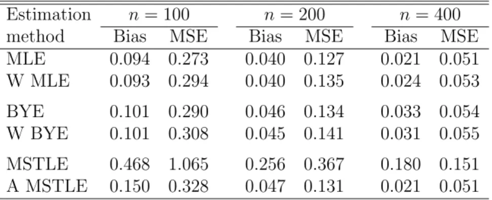
down-Table 1: Bias and MSE of all methods for data CLEAN using p = 2 variables and sample sizes n = 100,200, and 400.
Estimation n = 100 n= 200 n= 400
method Bias MSE Bias MSE Bias MSE
MLE 0.094 0.273 0.040 0.127 0.021 0.051 W MLE 0.093 0.294 0.040 0.135 0.024 0.053 BYE 0.101 0.290 0.046 0.134 0.033 0.054 W BYE 0.101 0.308 0.045 0.141 0.031 0.055 MSTLE 0.468 1.065 0.256 0.367 0.180 0.151 A MSTLE 0.150 0.328 0.047 0.131 0.021 0.051
weight all distant observations, is frequently used in the case of M-estimators (e.g., Gervini 2005).
As BYE is currently implemented only for logit, we compare all methods using a logistic model. In the case of simulated data, we generate pexplanatory variables
x1, . . . , xp ∼N(0,1), and for a given parameter vector β= (β0, β1, β2,0, . . . ,0)>, we define y=I(β0+β1x1+β2x2+ε≥0), whereε∼Λ(0,1) (N(µ, σ) and Λ(µ, s) refer to the Gaussian and logistic distributions, respectively). If a generated data set is not further modified, we refer to it as CLEAN. Next, to examine robust properties of all estimators, we also use contaminated data: a given fraction α ∈ (0,1) of observations is shifted by (∆1,∆2) ∈ R2 and misclassified, which corresponds to transformations x∗
1 = x1 + ∆1, x∗2 = x2 + ∆2, and y∗ = I(β0 +β1x∗1 +β2x∗2 < 0). Such data sets are referred to as OUTLIERS(α; ∆1,∆2).
Finally, let us note that the simulated results discussed in this section are ob-tained for β0 = 0.5, β1 = 1, and β2 = −1 using sample sizes n = 100,200, and 400 and 500 simulations. The MSTLE estimator is computed using the trimming constant hn = [0.75n] and the adaptive MSTLE estimator chooses the trimming parameter λ ∈ {0.66,0.70,0.75,0.80,0.85,0.90,0.95,1.00}.
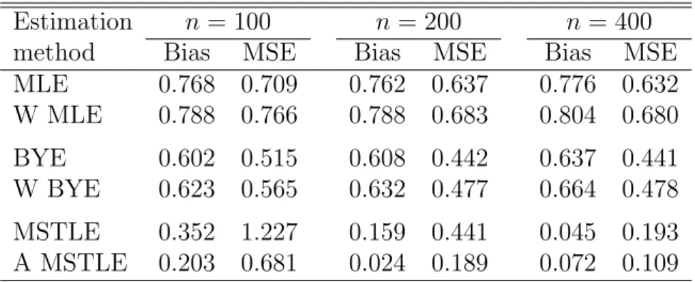
Table 2: Bias and MSE of all methods for data OUTLIERS(0.05; 1.5, -1.5) using
p= 2 variables and sample sizes n = 100,200, and 400.
Estimation n = 100 n= 200 n= 400
method Bias MSE Bias MSE Bias MSE
MLE 0.768 0.709 0.762 0.637 0.776 0.632 W MLE 0.788 0.766 0.788 0.683 0.804 0.680 BYE 0.602 0.515 0.608 0.442 0.637 0.441 W BYE 0.623 0.565 0.632 0.477 0.664 0.478 MSTLE 0.352 1.227 0.159 0.441 0.045 0.193 A MSTLE 0.203 0.681 0.024 0.189 0.072 0.109
4.1. Estimation with no contamination
The performance of all methods is first analyzed for data CLEAN, which are not contaminated by misclassified observations. The absolute values of bias and mean squared error (MSE) for each method are recorded in Table 1. For such data, MLE is the optimal estimation method as is confirmed by the simulations at all sample sizes: both the bias and MSE of MLE are minimal. The performance of MLE is closely matched by its weighted form and also by the (W)BYE estimators. On the other hand, MSTLE exhibits both a sizeable bias and large MSE (as expected). In contrast to this, the adaptive MSTLE is, in terms of MSE, slightly worse than (W)MLE and (W)BYE forn = 100, outperforms all methods but MLE forn = 200, and becomes identical to MLE at n = 400. The behavior of all methods is similar also for a more complex model with p= 12 variables, see Table 5 in Appendix C.
4.2. Estimation under contamination
All methods are now compared for contaminated data sets, where 5% observations are misclassified distant observations. Two cases, OUTLIERS(0.05; 1.5,−1.5) and
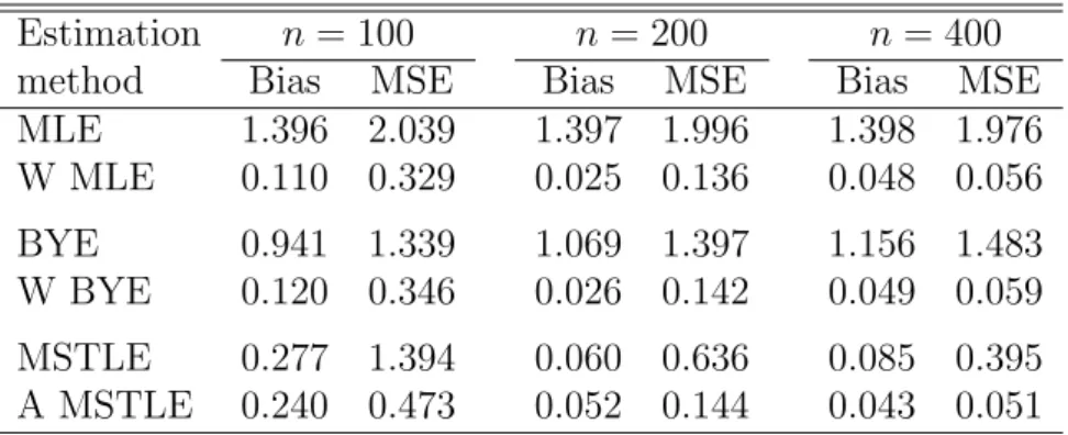
Table 3: Bias and MSE of all methods for data OUTLIERS(0.05; 5.0, -5.0) using
p= 2 variables and sample sizes n = 100,200, and 400.
Estimation n = 100 n= 200 n= 400
method Bias MSE Bias MSE Bias MSE
MLE 1.396 2.039 1.397 1.996 1.398 1.976 W MLE 0.110 0.329 0.025 0.136 0.048 0.056 BYE 0.941 1.339 1.069 1.397 1.156 1.483 W BYE 0.120 0.346 0.026 0.142 0.049 0.059 MSTLE 0.277 1.394 0.060 0.636 0.085 0.395 A MSTLE 0.240 0.473 0.052 0.144 0.043 0.051
OUTLIERS(0.05; 5.0,−5.0), are considered that differ by the distance of outlying observations from the rest of the data. We refer to the two cases as data with near outliers and data with distant outliers, respectively. The absolute values of bias and mean squared error (MSE) for both experiments are in Tables 2 and 3, respectively. In the case of data with near outliers, the MSE of all methods, but MSTLE, are similar at n = 100, although their large values have different sources – large bias in the cases of (W)MLE and (W)BYE and large variance in the case of the adaptive MSTLE. As the sample size increases, the biases and MSEs of (W)MLE and (W)BYE remains approximately on the same levels, whereas both measures significantly decrease in the case of (A)MSTLE. The adaptive MSTLE is thus the best performing method in this case since WMLE and WBYE are not able to detect and withstand this type of contamination at all.
The situation is different in the case of data with distant outliers. Even though MLE and BYE are extremely biased, their weighted versions WMLE and WBYE exhibit relatively small bias and MSE because the outlying points are now severely downweighted due to their distance from the rest of the data in the space of the explanatory variables. The adaptive MSTLE method, that does not a priori remove
0 20 40 60 80 100
0
1
White blood cell count (thousands)
Survived more than one year
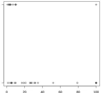
Figure 1: Data on 33 leukemia patients; symbol ‘+’ represents AG positive patients, whereas ‘◦’ stands for AG negative patients.
observations due to their position in the space, performs worse than WMLE at
n = 100, but closely matches the performance of the weighted methods atn = 200, and slightly outperforms WMLE and WBYE at n= 400.
The presented simulation results are representative also for higher levels of con-tamination (see Tables 7 and 9 in Appendix C) as well as for models with more explanatory variables (see Tables 6 and 8 in Appendix C).
4.3. Application
Let us now compare the (W)MLE, (W)BYE, and adaptive MSTLE using data on 33 leukemia patients. This data set, studied for example by Cook and Weisberg (1992)
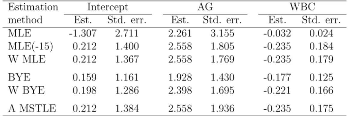
Table 4: Parameter estimates by all methods for the leukemia data. Estimate MLE(-15) represents the MLE estimate for the data without the 15th observation.
Estimation Intercept AG WBC
method Est. Std. err. Est. Std. err. Est. Std. err. MLE -1.307 2.711 2.261 3.155 -0.032 0.024 MLE(-15) 0.212 1.400 2.558 1.805 -0.235 0.184 W MLE 0.212 1.367 2.558 1.769 -0.235 0.179 BYE 0.159 1.161 1.928 1.430 -0.177 0.125 W BYE 0.198 1.286 2.398 1.695 -0.221 0.166 A MSTLE 0.212 1.384 2.558 1.936 -0.235 0.175
and Kordzakia et al. (2001), indicate whether a patient survives longer than one year (dependent variable yi = 1) conditional on the white blood cell count (measured in thousands, variable WBC) and a dichotomous morphological factor AG. Data are depicted on Figure 1, where we can observe that the chance to survive more than one year decreases with high values of WBC. Moreover, there is one extreme data point (observation 15) for a patient living longer than one year despite his WBC value being equal to 100 (other AG positive patients with WBC values above 50 did not survive longer than 5 weeks; see Feigl and Zelen 1965). This could possibly be due to some other unobservable physiological conditions of that particular patient. To provide a benchmark for comparing various estimators, we compute the MLE estimates both for the whole data and for data without the 15th observation. To-gether with (W)MLE, (W)BYE, and the adaptive MSTLE, all estimates are pre-sented in Table 4. The corresponding standard errors are obtained by a parametric bootstrap (using 10000 replications) because of the small sample size.
First, let us observe that, for the parameter WBC, the MLE estimate based on all data is more than 7 times smaller than the MLE estimate after omission of the 15th observation. Next, the WMLE and adaptive MSTLE with adaptively chosen
trimmingh∗ = 31 = [0.95·33] provide the same estimates as MLE after omitting the
15th observation, although they have slightly smaller of WBC estimate. Note that rather small standard errors of the adaptive MSTLE relative to results previously achieved in simulations likely come from the fact that trimming occurs here only on one side of data, that is, for large values of WBC (see Figure 1). Finally, although the WBYE estimates are rather close to those by WMLE and adaptive MSTLE, both BYE and WBYE seem to exhibit a downward bias since all their coefficients are 0.75 and 0.94 multiples of (W)MLE, respectively.
5. CONCLUSION
The adaptive maximum symmetrically-trimmed likelihood estimator proposed in this paper is shown to be generally applicable in binary-choice models, robust to various kinds of contamination, and at the same time, asymptotically efficient under no contamination. The combination of these properties is not currently matched by any other existing robust method in the context of the binary-choice regression. Moreover, the proposed methods allows the use of a robust estimation procedure without sacrificing the quality of estimation, especially at larger samples.
Further improvements could be obtained by replacing the hard (complete) re-jection of observations in MSTLE by weighting, which could then be determined in a data-adaptive way similar to the data-adaptive choice of trimming. Another interesting field of study is a combination of the adaptive MSTLE procedure with the MLE methods accounting for data misclassification (e.g., Hausman et al. 1998). Finally, the principle of the adaptive MSTLE estimation can be also applied to semi-parametric likelihood estimators (e.g., Klein and Spady 1993) under monotonicity constraint.
A. Assumptions
Further regularity assumptions used in Section 3.
Assumptions
4. The parameter space B is compact.
5. The mixing coefficientsbm of the sequence {xi, yi}i∈N satisfy
mr/(r−2)(logm)2(r−1)/(r−2)b m →0
for m→ ∞ and some r >2.
6. Expectation Esupβ∈B|l(xi, yi;β)|r is finite. 7. Expectation Esupβ∈U(β0,δ)|l0(x
i, yi;β)|r is finite for some δ >0. 8. Expectation Esupβ∈U(β0,δ)|l00(x
i, yi;β)|1+ε is finite for some δ >0 and ε >0.
B. Proofs
Proof of Lemma 1. Let us first derive an auxiliary results concerning function
h(t) = tlnt + (1− t) ln(1−t) for t ∈ (0,1). Taking its first derivative leads to
h0(t) = lnt−ln(1−t), which is negative fort <1/2 and positive fort >1/2. Hence,
h(t) is decreasing for t <1/2 and increasing for t >1/2 (property P1). Now, the conditional expectation to analyze can be rewritten as
E[l(xi, yi;β0)|r(xi;β0)≥C]
= E£yilnF(xi>β0) + (1−yi) ln{1−F(x>i β0)}|r(xi;β0)≥C
¤
= E£E(yi|xi) lnF(x>i β0) +{1−E(yi|xi)}ln{1−F(x>i β0)}|r(xi;β0)≥C
= E£F(x>
i β0) lnF(x>i β0) +{1−F(x>i β0)}ln{1−F(x>i β0)}|r(xi;β0)≥C
¤ .
Denoting random variablet=F(x>
i β0), it follows that the trimming ruler(xi,β0) = min{lnt,ln(1−t)} and we can write
E[l(xi, yi;β0)|r(xi;β0)≥C]
= E[tlnt+ (1−t) ln(1−t)|min{t,1−t} ≥exp(C)].
Because condition min{t,1− t} ≥ exp(C) means that t ∈ hexp(C),1−exp(C)i for exp(C) ≤ 1/2 and increasing C shrinks this interval, property P1 implies that
E[tlnt+ (1−t) ln(1−t)|min{t,1−t} ≥exp(C)] is non-increasing in C. Hence, the result of the lemma follows from the fact that the order statisticsr[n−hn+1](xi;β0) decreases as hn increases. ¤
Proof of Theorem 1. As discussed in Croux et al. (2002), an estimator of a binary-choice regression model can break down under contamination in two ways: either the estimates diverge and become infinite or they converge to a non-random zero vector. Assuming that the MLE estimate is identified, that is, there is an overlap in data, an estimator based on the likelihood criterion cannot diverge since some likelihood contributions would become infinite (see Croux et al. 2002, Theorem 1). Therefore, we only have to deal with the breakdown to a zero vector.
The adaptive MSTLE just chooses the amount of trimming λ on a grid 2/3 =
λ1 < . . . < λM = 1. Hence, we only have to show that the adaptive procedure selects a MSTLE estimator that does not break down. Considering a sample of size
n and the number of contaminated observationsk such that k/n≤maxm=1,...,Mεmn, there are sequences of samples with k additional (contaminated) observations such that the norm of the corresponding MSTLE estimate converges to 0 if k/n > εm n
and stays bounded away from 0 for any such sequence if k/n ≤εm
n; m = 1, . . . , M. To verify the claim of the theorem, we thus have to show that the selection criterion at an MSTLE estimate βˆm, which does not break down,
S(hm n,βˆ m ) = 1 hm n n X j=1 l(xi, yi;βˆ m )·I ³ r(xi;βˆ m )≥r[n−hm n+1](xi;βˆ m ) ´ , (6)
is larger than the selection criterion at kβk= 0.
To prove this, note that the selection criterion (6) is independent ofhnifkβk= 0 because l(xi, yi; 0) = ln(1/2). If we now consider trimming hmn such that k/n≤εmn, the corresponding MSTLE estimate βˆm does not break down and stays bounded away from 0. Since βˆm maximizes the trimmed likelihood (5), and thus, for a fixed hm
n, also the selection criterion (6), S(hmn,βˆ m
) > S(hm
n,0) = S(h,0) for any
h= [n/2], . . . , n. ¤
Proof of Theorem 2. The asymptotic normality of MSTLE directly follows from ˇ
C´ıˇzek (2007, Theorem 3.3), where most distributional and functional assumptions of the theorem are parts of Assumptions 1–8. The exceptions are the identification assumptions, which are verified in ˇC´ıˇzek (2007, Section 4.3) under Assumption 1–8, and assumptions that F0 ={r(xi;β)|β ∈ B} and F1 ={l0(xi, yi;β)|β ∈U(β0, δ)} form VC classes of functions, which are verified in the following paragraphs.
First, note thatr(xi;β) = min{lnF(x>i β),ln[1−F(x>i β)]}. Since{x>i β|β∈B} is (a part of) a finite dimensional vector space and lnF is a monotonic function, F0 is a VC class of functions (van der Waart and Wellner 1996, Lemmas 2.6.15 and 2.6.18).
Second, the derivative l0(x
i, yi;β) of the likelihood contribution equals to
l0(x i, yi;β) = yif(x>i β) F(xi>β) − (1−yi)f(x > i β) 1−F(xi>β)
= (2yi−1) max ½ yif(x>i β) F(x> i β) ,(1−yi)f(x > i β) 1−F(x> i β) ¾ ,
see (3). Because functions f /F and f /(1−F) are derivatives of concave functions lnF and ln(1−F), respectively, they are monotonic. Hence, F1 is a VC class of functions by the same argument as above (van der Waart and Wellner 1996, Lemmas 2.6.15 and 2.6.18). ¤
Proof of Theorem 3. The selection criterion determining the optimal amount of trimming can be expressed as
Cm = 1 hm n n X j=1 l(xi, yi;βˆ m )·I ³ r(xi;βˆ m )≥r[n−hm n+1](xi;βˆ m ) ´ . (7)
By Theorem 2, the βˆm → β0 for all m = 1, . . . , M. This implies that the order statistics r[n−hm
n+1](xi;βˆ
m
) → R−1(1− λ
m) ( ˇC´ıˇzek 2007, Lemma A.2), where R denotes the distribution function of r(xi;β0). Note that, by Assumption 3, R is absolutely continuous, and by definition, R−1(1−λ
m) > R−1(1−λM) for m < M since λM = 1.
An immediate consequence is that, by Lemma 1 and Assumption 3, expectation
Em =E
£
l(xi, yi;β0)|r(xi;β0)≥R−1(1−λm)
¤
as a function of m has a unique maximum at m=M (λM = 1). Since ˇC´ıˇzek (2007, Lemma A.1) implies that the average (7) converges to Em uniformly inm, one can find for any ε > 0 some n0 ∈ N such that |Cm −Em| < (EM − EM−1)/2 with probability higher than 1−ε, which implies P(m∗
n =M) ≥ 1−ε for any n > n0. Thus,m∗
n →M in probability, and consequently,λm∗
Therefore, √ n(βˆ(AM ST LE)−β0) = M X m=1 √ n(βˆ(M ST LE,[λmn])−β0)I(m =m∗ n) = √n(βˆ(M ST LE,n)−β0) +oP(1)
C. Further simulation results
Table 5: Bias and MSE of all methods for data CLEAN using p= 12 variables and sample sizes n = 100,200, and 400.
Estimation n = 100 n = 200 n = 400
method Bias MSE Bias MSE Bias MSE
MLE 0.333 1.423 0.125 0.464 0.046 0.190 W MLE 0.385 1.886 0.114 0.499 0.044 0.205 BYE 0.454 1.921 0.142 0.498 0.057 0.203 W BYE 0.760 2.821 0.138 0.540 0.056 0.222 MSTLE 2.384 11.275 0.828 2.215 0.443 0.646 A MSTLE 0.981 4.330 0.193 0.568 0.046 0.190
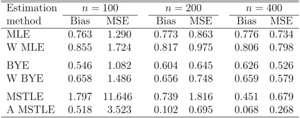
Table 6: Bias and MSE of all methods for data OUTLIERS(0.05; 1.5, -1.5) using
p= 12 variables and sample sizes n= 100,200,and 400.
Estimation n = 100 n = 200 n = 400
method Bias MSE Bias MSE Bias MSE
MLE 0.763 1.290 0.773 0.863 0.776 0.734 W MLE 0.855 1.724 0.817 0.975 0.806 0.798 BYE 0.546 1.082 0.604 0.645 0.626 0.526 W BYE 0.658 1.486 0.656 0.748 0.659 0.579 MSTLE 1.797 11.646 0.739 1.816 0.451 0.679 A MSTLE 0.518 3.523 0.102 0.695 0.068 0.268
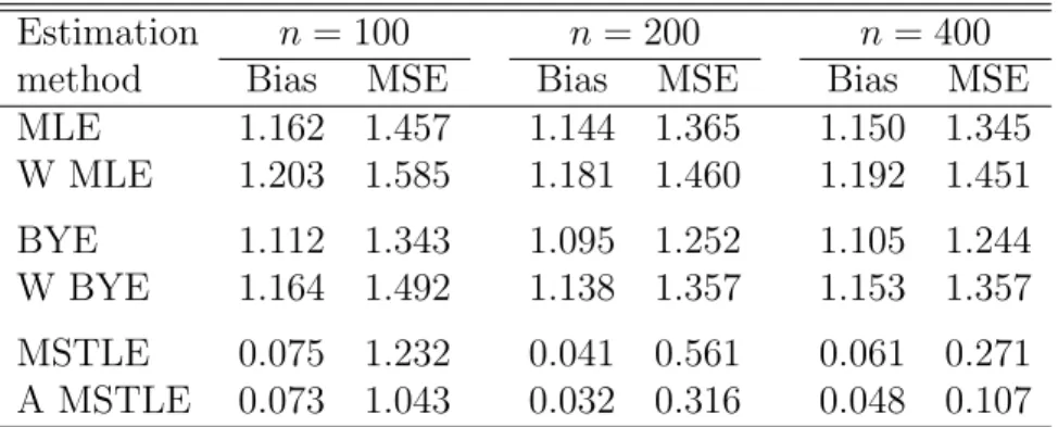
Table 7: Bias and MSE of all methods for data OUTLIERS(0.10; 1.5, -1.5) using
p= 2 variables and sample sizes n = 100,200, and 400.
Estimation n = 100 n= 200 n= 400
method Bias MSE Bias MSE Bias MSE
MLE 1.162 1.457 1.144 1.365 1.150 1.345 W MLE 1.203 1.585 1.181 1.460 1.192 1.451 BYE 1.112 1.343 1.095 1.252 1.105 1.244 W BYE 1.164 1.492 1.138 1.357 1.153 1.357 MSTLE 0.075 1.232 0.041 0.561 0.061 0.271 A MSTLE 0.073 1.043 0.032 0.316 0.048 0.107
Table 8: Bias and MSE of all methods for data OUTLIERS(0.05; 5.0, -5.0) using
p= 12 variables and sample sizes n= 100,200,and 400.
Estimation n = 100 n = 200 n = 400
method Bias MSE Bias MSE Bias MSE
MLE 1.421 2.708 1.408 2.268 1.396 2.076 W MLE 0.367 2.011 0.141 0.566 0.099 0.255 BYE 0.841 2.218 1.022 1.595 1.009 1.349 W BYE 0.447 2.024 0.172 0.627 0.115 0.278 MSTLE 1.751 11.665 0.713 2.017 0.429 0.750 A MSTLE 0.897 3.981 0.289 0.764 0.145 0.286
Table 9: Bias and MSE of all methods for data OUTLIERS(0.10; 5.0, -5.0) using
p= 2 variables and sample sizes n = 100,200, and 400.
Estimation n = 100 n= 200 n= 400
method Bias MSE Bias MSE Bias MSE
MLE 1.562 2.546 1.559 2.481 1.557 2.443 W MLE 0.106 0.323 0.053 0.148 0.038 0.043 BYE 1.555 2.533 1.552 2.462 1.550 2.422 W BYE 0.123 0.352 0.055 0.159 0.040 0.043 MSTLE 0.259 2.269 0.377 1.507 0.156 0.621 A MSTLE 0.248 1.714 0.099 0.208 0.035 0.042
References
[1] Albert, A., and Anderson, J. A. (1984), “On the existence of maximum likeli-hood estimates in logistic regression models,” Biometrika, 71, 1–10.
[2] Bianco, A. M., and Yohai, V. J. (1996), “Robust estimation in the logistic regression model,” in Robust statistics, data analysis, and computer intensive methods, ed. H. Rieder, New York: Springer, 17–34.
[3] Carroll, R. J., and Pederson, S. (1993), “On robustness in the logistic regression model,” Journal of Royal Statistical Society, Ser. B, 55, 693–706.
[4] Christmann, A. (1994), “Least median of weighted squares in logistic regression with large strata,” Biometrika, 81, 413–417.
[5] Christmann, A., and Rousseeuw, P. J. (2001), “Measuring overlap in binary regression,” Computational Statistics and Data Analysis, 37, 65–75.
[6] ˇC´ıˇzek, P. (2005), “Least trimmed squares in nonlinear regression under depen-dence,” Journal of Statistical Planning and Inference, 136, 3967–3988.
[7] ˇC´ıˇzek, P. (2006), “Trimmed likelihood-based estimation in binary regression models,” Austrian Journal of Statistics, 35, 223–232.
[8] ˇC´ıˇzek, P. (2007), “General trimmed estimation: robust approach to nonlinear and limited dependent variable models,” CentER Discussion Paper 2007/1, Tilburg University; submitted to Econometric Theory.
[9] Cook, R. D., and Weisberg, S. (1982), Residuals and Influence in Regression, London: Chapman and Hall.
[10] Copas, J. B. (1988), “Binary regression models for contamination data,” Jour-nal of Royal Statistical Society, Ser. B, 50, 225–265.
[11] Croux, C., Flandre, C., and Haesbroeck, G. (2002), “The breakdown behavior of the maximum likelihood estimator in the logistic regression model,”Statistics and Probability Letters, 60, 377–386.
[12] Croux, C., and Haesbroeck, G. (2003), “Implementing the Bianco and Yohai estimator for logistic regression,” Computational Statistics and Data Analysis, 44, 273–295.
[13] Feigl, P., and Zelen, M. (1965), “Estimation of exponential survival probabilities with concomitant information,” Biometrics, 21, 826–838.
[14] Genton, M. G., and Lucas, A. (2003), “Comprehensive definitions of break-down points for independent and dependent observations,” Journal of Royal Statistical Society, Ser. B, 65, 81–94.
[15] Gervini, D. (2005), “Robust adaptive estimators for binary regression models,”
Journal of Statistical Planning and Inference, 131, 297–311.
[16] Hadi, A., and Luce˜no, A. (1997), “Maximum trimmed likelihood estimators: a unified approach, examples and algorithms,” Computational Statistics and Data Analysis, 25, 251–272.
[17] Hall, P., and Presnell, B. (1999), “Biased bootstrap methods for reducing the effects of contamination, ” Journal of Royal Statistical Society, Ser. B, 61, 661–680.
[18] Hausman, J. A., Abrevaya, J., and Scott-Morton, F. M. (1998), “Misclassi-fication of the dependent variable in a discrete-response setting,” Journal of Econometrics, 87, 239–269.
[19] Kordzakhia, N., Mishra, G. D., and Reiersølmoen, L. (2001), “Robust esti-mation in the logistic regression model,” Journal of Statistical Planning and Inference, 98, 211–223.
[20] Klein, R. W., and Spady, R. H. (1993), “An efficient semi-parametric estimator for binary response models,” Econometrica, 61, 387–421.
[21] M¨uller, C. H., and Neykov, N. M. (2003), “Breakdown points of trimmed like-lihood estimators and related estimators in generalized linear models,” Journal of Statistical Planning and Inference, 116, 503–519.
[22] Pregibon, D. (1981), “Logistic regression diagnostics,”The Annals of Statistics, 9, 705–724.
[23] Salibian-Barrera, M., and Zamar, R. H. (2002), “Bootstrapping robust esti-mates of regression,” The Annals of Statistics, 30, 556–582.
[24] Silvapulle, M. J. (1981), “On the existence of maximum likelihood estimates for the binomial response models,” Journal of Royal Statistical Society, Ser. B, 43, 310–313.
[25] Stromberg, A. J., and Ruppert, D. (1992), “Breakdown in nonlinear regression,”
Journal of American Statistical Association, 87, 991–997.
[26] Van der Vaart, A. W., and Wellner, J. A. (1996), Weak convergence and em-pirical processes: with applications to statistics, New York: Springer.