A generic framework for stochastic Loss-Given-Default

Contents lists available atScienceDirect

Journal of Computational and Applied

Mathematics

journal homepage:www.elsevier.com/locate/cam

A generic framework for stochastic Loss-Given-Default

Geert Van Damme

Katholieke Universiteit Leuven, Leuven, Belgium

a r t i c l e i n f o

Article history:

Received 10 February 2010

Received in revised form 31 October 2010

Keywords: Loss-Given-Default Lévy process Factor model Basel II

a b s t r a c t

In this document a method is discussed to incorporate stochastic Loss-Given-Default (LGD) in factor models, i.e. structural models for credit risk. The general idea exhibited in this text is to introduce a common dependence of the LGD and the probability of default (PD) on a latent variable, representing the systemic risk. Though our theory can be applied to any arbitrary firm-value model and any underlying distribution for the LGD, provided its support is a compact subset of[0,1], special attention is given to the extension of the well-known cases of the Gaussian copula framework and the shifted Gamma one-factor model (a particular case of the generic one-factor Lévy model), and the LGD is modeled by a Beta distribution, in accordance with rating agency models and the Credit Metrics model.

In order to introduce stochastic LGD, a monotonically decreasing relation is derived between the loss rateL, i.e. the loss as a percentage of the total exposure, and the standardized log-returnRof the obligor’s asset value, which is assumed to be a function of one or more systematic and idiosyncratic risk factors. The property that the relation is decreasing guarantees that the LGD is negatively correlated toRand hence positively correlated to the default rate. From this relation, expressions are then derived for the cumulative distribution function (CDF) and the expected value of the loss rate and the LGD, conditionally on a realization of the systematic risk factor(s). It is important to remark that all our results are derived under the large homogeneous portfolio (LHP) assumption and that they are fully consistent with the IRB approach outlined by the Basel II Capital Accord.

We will demonstrate the impact of incorporating stochastic LGD and using models based on skew and fat-tailed distributions in determining adequate capital requirements. Furthermore, we also skim the potential application of the proposed framework in a credit risk environment. It will turn out that both building blocks, i.e. stochastic LGD and fat-tailed distributions, separately, increase the projected loss and thus the required capital charge. Hence, the aggregation of a model based on a fat-tailed underlying distribution that accounts for stochastic LGD will lead to sound capital requirements.

©2010 Elsevier B.V. All rights reserved.

1. Introduction

For long time, researchers and practitioners in the field of (portfolio) credit risk have spent more time and resources on modeling default risk and default dependence than they have on what is called Loss-Given-Default (LGD). According to the Basel II Capital Accord, LGD is the fraction of Exposure-At-Default (EAD) that will not be recovered following default. Traditional pricing and rating models generally combine a stochastic, or at least dependent, default rate with a time-invariant and constant LGD. For instance, even now, index and single name traders are still using a fixed 40% recovery

E-mail address:[email protected].

0377-0427/$ – see front matter©2010 Elsevier B.V. All rights reserved.

assumption for their present value calculations, which causes problems in the CDO context, where the newly emerging [60%, 100%] super duper tranche would have1_{no value under traditional models.}

Moreover, the financial crises of the past decade and their devastating impact on the global economy provided empirical evidence for the existence of significant positive correlation between the default rate and the LGD in a specific period (cf. [1]). This has led to the consensus that the current models are inadequate, calling for new methods taking into account non-constant LGD. Under Basel II, for instance, banks and other financial institutions are now recommended to calculate the Downturn LGD, which reflects economic downturn conditions where necessary to capture the relevant risks, i.e. the realized recovery rates should be lower than average during times of high default rates, to avoid underestimating the expected loss (cf. Basel Committee on Banking [2,3]). The main reason for this requirement is that the Vasicek model (cf. [4]) used in the Basel Capital Accord does not have systematic correlation between probability of default (PD) and loss given default (LGD), which would underestimate downturn risk.

In the literature, several ways have yet been proposed to obtain a non-constant LGD that is correlated with the default risk, extending each of the three popular approaches for modeling default risk, i.e. reduced form models, firm-value models and the copula approach. The former two approaches model the LGD by assuming it is driven by a latent variable that is correlated with the latent variable driving default (cf. [5–7]), whereas the latter aim at directly modeling the spot recovery, i.e. the recovery upon default (cf. [8,9]). An extensive overview of the literature can be found in [10].

In this document a method is discussed to incorporate stochastic LGD in structural models for default risk, as introduced in the seminal papers in [11,12], by introducing a common dependence of the LGD and the PD on a latent variable, representing the systemic risk. Though our theory can be applied to any arbitrary firm-value model and any underlying distribution for the LGD, provided its support is a compact subset of

[

0

,

1

]

, special attention is given to the extension of the well-known cases of the Gaussian copula framework and the shifted Gamma factor model, i.e. a particular case of the generic one-factor Lévy model (cf. [13]). Furthermore in this text, w.r.t. the above implementations, we will model the LGD by a Beta distribution, in line with rating agency models and the Credit Metrics model.

In order to introduce stochastic LGD, a monotonically decreasing relation is derived between the loss rateL, i.e. the loss as a percentage of the total exposure, and the standardized log-returnRof the obligor’s asset value, which is assumed to be a function of one or more systematic and idiosyncratic risk factors. As a starting point, we use the work of Tasche [6] and Joocheol et al. [7]. The property that the relation is decreasing, guarantees that the LGD is negatively correlated toRand hence positively correlated to the default rate. From this relation, expressions are next derived for the cumulative distribution function (CDF) and the expected value of the loss rate and the LGD, conditionally on a realization of the systematic risk factor(s). It is important to remark that all our results are derived under the large homogeneous portfolio (LHP) assumption and that they are fully consistent with the IRB approach outlined by the Basel II Capital Accord.

We will demonstrate the impact of incorporating stochastic LGD and using models based on skew and fat-tailed distributions in determining adequate capital requirements. Furthermore, we also skim the potential application of the proposed framework in a credit risk environment. It will turn out that both building blocks, i.e. stochastic LGD and fat-tailed distributions, separately, increase the projected loss and thus the required capital charge. Hence, the aggregation of a model based on a fat-tailed underlying distribution that accounts for stochastic LGD will lead to sound capital requirements.

The text is organized as follows: Section2describes the general framework. We determine a relation between the loss rateLand the standardized log-returnRof the debtor’s asset value and, based on this relation, derive expressions for the CDF and the expected value of the loss rateLand the LGD, conditionally on a level of the systematic risk. Sections3and4discuss the extensions of the Normal factor model and the generic factor Lévy model, especially the (shifted) Gamma one-factor model. Section5forms the main contribution of this text and provides a generalization, allowing the loss rateLto depend on two risk drivers instead of one, breaking the comonotonicity between defaults and losses that is introduced by the relation described in Section2. In Section6we demonstrate the impact of accounting for downturn (stochastic) LGD on the capital charge required under the Basel II Capital Accord and compare our model with the work of Amraoui and Hitier [14] and Andersen and Sidenius [10], who introduce stochastic LGD in structural models for CDO valuation, with the aim of flattening the base-correlation curve. Section7concludes the paper. Readers interested only in a specific formula, may skip the text and go straight to theAppendixat the end, where all the results are summarized.

2. General framework 2.1. Introduction

In this section we develop the general framework. Starting from a structural model for credit risk and under the large homogeneous portfolio (LHP) assumption, we will derive a model-independent relation between the cumulative loss rate Lt, i.e. the loss as a percentage of the total exposure, and the standardized log-returnRof the obligor’s asset value. Moreover, we will show that the results derived in this section are fully consistent with the Basel II framework.

Consider a portfolio with notional value N, consisting of M names with respective notionals Ni

,

i

=

1

, . . . ,

M. Furthermore, assume thatCis a macro-economic factor, common to all credits and thatIiis an idiosyncratic factor, specific 1 Assuming a fixed 40% recovery, i.e. a fixed 60% LGD, the expected loss (and hence the value) of the [60%, 100%] super duper tranche will be equal to zero.

to theith name. Finally, let

ρ

∈

(

0

,

1

)

denote the correlation between the log-returns of any two namesiandj

̸=

i, i.e. we assume equicorrelation between the log-returns. Following2_{Merton’s model, obligoridefaults in a time period}

[

₀

,

_t

]

_{if the}

standardized log-return of the asset valueRi not.

=

Ri

(

C

,

Ii

;

ρ)

hits a certain lower boundHtd, that is 1di,t

=

1

⇔

Ri

≤

Htd, with 1d

i,tthe default indicator, equaling 1 if theith name has defaulted in the interval

[

0

,

t

]

and 0 otherwise. Furthermore, the corresponding default probability (PD) is given bypd

i,t

=

Pr



1d i,t

=

1



=

Pr



Ri

≤

Htd



. Mark thatRiis traditionally modeled by a Normal one-factor model, i.e.

Ri

=

√

ρ

C

+



1

−

ρ

Ii

,

where the random variablesCandIiare assumed to be i.i.d. and follow a standard Normal distribution. The latter Gaussian one-factor model will be covered in Section3. However, as mentioned before, in Section4of this text we will also examine the possibilities of incorporating stochastic LGD in the (shifted) Gamma one-factor model (cf. [13]). Though it should be mentioned that the different models discussed in this text are consistent w.r.t.

ρ

, in the sense that they all satisfy Corr



Ri

,

Rj



=

ρ

, fori

̸=

j

,

Corr [Ri

,

C]

=

√

ρ

and Corr [Ri

,

Ii]

=

√

1

−

ρ

.

Any default by an arbitrary credit induces a loss to the investor. The fraction of the Exposure-At-Default (EAD) that will not be recovered in the event of a default is referred to as the Loss-Given-Default (LGD). To clarify this, letPLi,tdenote the cumulative loss due to creditiuntil timet. Furthermore, assume that the PD3_{at timetis stochastic and given byQ}d

i,t, where E



Qd i,t



=

pd

i,t. Finally, note that the loss is only positive in the case of a default. Then, the cumulative portfolio loss rate, i.e. the total loss as a percentage of the total exposure, until timet, is given by

Lt

=

PLt N

=

1 N M

−

i=1 PLi,t

=

1 N M

−

i=1



Li,t





1d_i,t

=

1



Q_id_,tNi

,

withLi,tthe cumulative loss rate at timetof a fixed obligori. Denote the LGD of obligoriby LGDi,t

=



Li,t





1d_i,t

=

1



. In the sequel we assume that the LGD is time-independent and omit the subscriptt.

Now, under the LHP assumption, it holds thatQ_id_,t

=

d Qd

t and LGDiQid,t d

=

LGDQd

t, for alli

=

1

,

2

, . . . ,

M, such that PLt

d

=

LGDQ_tdN

,

(1)

where

=

d stands for equality in distribution. Hence, in the LHP limit, due to the strong Law of large numbers,Ltis equal to the expected loss of one obligor, i.e.

Lt

=

E



LGDQ_td



,

(2)

which is traditionally set equal to = E [LGD]pd

t, justified by the assumption that the LGD and the PD are independent, where, the LGD is generally assumed to be constant. However, as declared before, there is sufficient empirical evidence for the existence of significant positive correlation between the latter variables, in a specific time period (cf. [1]).

The latter obviously complicates the computation of the expectation in the right-hand side of(2). The general idea exhibited in this text is to introduce a common dependence of the LGD and the PD on the latent variableC, representing the systematic risk, while assuming independence of the conditional LGD (CLGD) and the conditional PD (CPD) (cf. [6,7]). More specifically, we will determine the conditional expected loss rate, conditional on a common factorCand set

Lt

=

κ(

C

)

=

E



LGDQ_td





C



=

E [LGD

|

C]pd_t,C

,

(3)

wherepd_t,C is the conditional expected default probability and

κ

a monotonically decreasing function ofC. This implies (cf. [17]) that Pr [Lt

≤

l]

=

Pr [

κ(

C

)

≤

l] ∗

=

1

−

Pr



C

≤

κ

[−1]

(

l

)



,

(4)

from which the Value-at-risk (VaR) can then be computed as VaR_α

(

Lt

)

=

κ



F_C[−1]

(

1

−

α)



.

(5)

Furthermore, the downturn LGD (DLGD) is defined as (cf. [18]) DLGD_α

=

VaRα

(

Lt

)

pd,F [−1] C (α) t

=

E



LGD







C

=

F [−1] C

(α)



,

(6)

2 In this work we assume Merton’s one-period model for default, i.e. default can only occur at the maturityTof the debt instrument. This has some obvious drawbacks, as compared to the first-passage models (cf. [15]) allowing default to occur at any timet∈ [0,T]. However, this issue can easily be solved by introducing a time-dependent default barrier (cf. [16]).

withF_X[−1] the generalized inverse of the CDF of a random variable X. The second equality of(6)follows directly from substituting(5)into(3). Note, however, that equality

=

∗ and therefore Eqs.(3)and(5)are only valid ifCis one-dimensional. Hence, ifCis a vector of 2 or more common factors (cf. Section5.4) there will generally be no other solution than to derive the VaR and DLGD through simulation, based on

κ(

C

)

and thus on the expected value of the CLGD. Therefore, in this text, we will primarily be concerned with the derivation of the latter quantity.

2.2. Model framework

We are now ready to derive the model-independent relation between the loss rate and the standardized log-returnRof the obligor’s asset value. Assume that

Lt

=



Λ

>

0

;

1d_t

=

1

;

0

;

1d_t

=

0

,

(7)

is the cumulative loss rate of an arbitrary name in the (homogeneous) portfolio. Notice that the random variableΛis in fact the (time-independent) LGD and is distributed according to a lawD, with bounded support

[

λ

_l

, λ

_u

]

, where 0

≤

λ

_l

≤

λ

_u

≤

1. A popular choice forDis the Beta

(

a

,

b

)

distribution, because the support of the latter is

[

0

,

1

]

. Moreover, we have that Pr [Lt

>

0]

=

Pr



1d t

=

1



=

pd

t. Hence, it holds that Pr [Lt

>

0]

=

Pr



R

≤

Hd t



, where the risk factorR not

=

.R

(

C

,

I

;

ρ)

is a function of a systematic risk factorCand an idiosyncratic risk factorI, satisfying Corr [R

,

C]

=

√

ρ,

Corr [R

,

I]

=

√

1

−

ρ

, and whereHd_{is the (possibly time dependent) default barrier, which triggers default when being hit byR.}

From the above it follows that (cf. [6]) pl,t

=

Pr [Lt

≤

l]

=

F_Λ

(

l

)

·

pd_t

+



1

−

pd_t



,

(8)

for alll

∈ [

0

,

1

]

and for allt

≥

0, withF_Λ

(

l

)

=

Pr



Lt

≤

l





1d_t

=

1



the CDF associated to the lawD. But this implies that

l

=











F_Λ[−1]



pl,t

−



1

−

pd t



pd_t



;

1

−

pd_t

<

pl,t

≤

1

;

0

;

0

≤

pl,t

≤

1

−

pd

,

withF_Λ[−1]the inverse of the CDF ofΛ. Using the fact that

∀

l

∈

(

0

,

1

]

,

∃!

r

∈



inf

(

R

),

H_td



:

pl,t

=

1

−

FR

(

r

)

, leads to Lt

=

h1(R

)

=







F_Λ[−1]



1

−

FR

(

R

)

pd t



;

inf

(

R

)

≤

R

<

H_td

;

0

;

H_td

≤

R

≤

sup

(

R

),

(9)

hence, forr

∈



inf

(

R

),

H_td



we have

r

=

h[−1]₁

(

l

)

=

F_R[−1]



[1

−

F_Λ

(

l

)

]pd_t



,

(10)

withl

∈

(

0

,

1]. By convention, we seth₁[−1]

(

0

)

=

F_R[−1]



pd t



=

Hd t. Notice that FR(R) pdt

=

Pr



R

≤

R





R

≤

H_td



not.

=

F R   R≤H d t

(

R

)

. From this it is easy to verify that

1

−

FR

(

R

)

pd t

=

1

−

F R   R≤H d t

(

R

)

=

F_Λ

(

Λ

)

∼

Un

[

0

,

1

]

,

(11) such thatF_Λ[−1]



1

−

FR(R) pdt



=

Λ, for inf

(

R

)

≤

R

<

H_td, as required. Furthermore, using(9)and(11), Eq.(10)can be rewritten as follows r

=

h[−1]₁

(

l

)

=

F[−1] R   R≤H d t

(

1

−

F_Λ

(

l

)) ,

l

∈

(

0

,

1]

.

(12)

Recall, from the previous paragraph, that we assumed the LGDΛto be time-independent, i.e. the parameters of the law Dare independent of the time of default. Moreover, we assume that the latter law is also independent of the distribution of the risk factorR.4However, the latter distribution will influence the conditional distribution of the LGD, conditional on a realization of the systematic risk factorCor the idiosyncratic risk factorI. In this paper we only examine the situation of

4 Unlike the distribution of the loss rateLt, which depends both on time and the underlying factor model, throughpdt, i.e. the unconditional probability

common dependence of the LGD and the PD on the systematic factorC, thereby following Joocheol et al. [7], who state that under the asymptotic single risk factor model the loss rate for a well diversified portfolio depends only on the (single) systematic risk factor and not on the idiosyncratic risk factors. Though the reader is cordially invited to translate the theory to conditioning onI.

Assuming a one-factor structural model for the obligor’s asset value, the conditional distribution of the LGD, givenC

=

c, is given by Pr



Lt

≤

l

|

R

≤

Htd

,

C

=

c



=

Pr



h1(R

)

≤

l





R

≤

H_td

,

C

=

c



∗

=

Pr



R

≥

h[−1]₁

(

l

)







R

≤

H d t

,

C

=

c



=

1

−

Pr



R

≤

h[−1]₁

(

l

)







C

=

c



Pr



R

≤

Hd t





C

=

c



,

(13)

where equality

=

∗ is explained by the fact that the functionh1is monotonically decreasing inR(cf.(9)). Now, if we denote the conditional CDF of the LGD givenC

=

cbyF_Λ|C=c

(

·

)

and the corresponding CPD bypdt,c, then, combining(8)and(13) yields that the conditional distribution of the loss rateL, givenC

=

c, satisfies

Pr [Lt

≤

l

|

C

=

c]

=

FΛ|C=c

(

l

)

·

pdt,c

+



1

−

pd_t,c



=

1

−

Pr



R

≤

h[−1]₁

(

l

)







C

=

c



.

(14)

Moreover, using relations(9)and(14), we can determine the expected value of the CLGD as E



Lt





R

≤

H_td

,

C

=

c



=

E [Lt

|

C

=

c] Pr



R

≤

Hd t





C

=

c



=



λu l=λlPr



R

≤

h[−1]₁

(

l

)







C

=

c



dl Pr



R

≤

Hd t





C

=

c



.

(15)

Note that the numerator in the right-hand side of the above expression equals

κ(

c

)

=

VaR1−FC(c)(cf.(3)and(5)), thus (15)corresponds to DLGD1−FC(c). Hence, being able to compute the above quantities allows one to incorporate stochastic recovery rates in VaR and DLGD calculations (cf.(5)and(6)), but it also has many other practical applications, e.g. as pricing models for credit defaults swaps (CDSs) or collateralized debt obligations (CDOs) and scenario generators for analyzing and rating asset-backed securities (ABSs).

Finally, note that(15)is in line with the standard procedure, outlined in the Basel II capital framework, of setting the expected loss rate equal to E [Lt]

=

E



Lt





1d_t

=

1



Pr



1d t

=

1



. Conditioning onC

=

cand dividing both sides of the latter equality by Pr



1d_t

=

1





C

=

c



leads to(15).

In the next two sections, following rating agency practice, we will assume thatΛfollows a Beta distribution, with parametersa

,

b

>

0, hence

λ

l

=

0 and

λ

u

=

1.5Though it should be kept in mind that any distribution with bounded support is suited forΛ.6_{Readers interested in the formulas for a general distribution are referred to theAppendixat the end}

of this text. Hence,

Lt

=

h1(R

)

=







B[−1]a,b



1

−

FR

(

R

)

pd t



;

inf

(

R

)

≤

R

<

H_td

;

0

;

H_td

≤

R

≤

sup

(

R

),

(16) and r

=

F_R[−1]



1

−

_Ba,b

(

l

)



pd_t



,

l

∈

(

0

,

1]

,

(17)

with_Ba,bthe CDF of the Beta distribution with parametersaandb. The latter can be calibrated based on historical data regarding the expected value and the variance of the loss rateLor the LGDΛ. However, assuming that 1

−

E

[

LGD

]

is equal to the expected recovery conditional on default, to be consistent with single-name and index pricing, the LGD model must be calibrated such that 1

−

E

[

LGD

]

is the same as the mid recovery, generally taken to be 40% w.r.t. CDSs (cf. [14]).

5 Letσ2

XandµXdenote the variance and the expected value of the random variableX, then it is easy to verify thatσL2t=p

d t  µ2 LGD+σ 2 LGD  − µLGDpd t 2 . By the properties of the Beta distribution, it then follows that 0≤µ2

LGDp d t  1−pd t  < σ2 L < µLGDp d t  1−µLGDpd t  ≤0.25.

6 Note that one can always construct a random variableYwith support[λl, λu]from a Beta(a,b)distributed random variableX, using the transformation

3. The Gaussian one-factor model

Recall that the Normal one-factor model models the asset valueVof a borrower, whereVis described by a geometric Brownian motion, VT

=

V0exp [

µ(

T

)

+

σ (

T

)

WT] d

=

V0exp



µ(

T

)

+

σ(

T

)

√

T Z



,

(18)

withWa Wiener process and where the random variableZ

∼

N

(

0

,

1

)

satisfies Znot

=

.R

(

X

, ξ

;

ρ)

=

√

ρ

X

+



1

−

ρξ,

withX

, ξ

i.

∼

i.d. N

(

0

,

1

)

and

ρ

∈

(

0

,

1

)

. The random variableXdenotes the systematic risk factor (C) which is common to each obligor and the random variable

ξ

represents the idiosyncratic risk factor (I) associated with each individual obligor. Finally, as indicated before,

ρ

determines the borrower’s exposure to the systematic and idiosyncratic risk factors.

A borrower is said to default at time t

≥

0, if his financial situation deteriorates so dramatically that VT hits a predetermined lower boundBd

t, which (as can be seen from(18)) is equivalent to saying thatZhits some barrierHtd

∈

R. From(16)it then follows that

Lt

=

h1(Z

)

=







B[−1]a,b



1

−

Φ

(

Z

)

Φ

(

H_td

)



;

−∞ ≤

Z

<

H_td

;

0

;

H_td

≤

Z

≤ +∞

,

(19)

henceh[−1]₁

(

l

)

=

Φ[−1]



1

−

_Ba,b

(

l

)



Φ



H_td



, forl

∈

(

0

,

1

]

, whereΦis the CDF of the standard Normal distribution. Using Eqs.(13)–(15)this leads to

Pr



Lt

≤

l





Z

≤

H_td

,

X

=

x



=

1

−

Φ

[

h[−₁ 1](l)−√ρx √ 1−ρ

]

Φ



Htd− √ ρx √ 1−ρ



,

(20) Pr [Lt

≤

l

|

X

=

x]

=

1

−

Φ



h[−1]₁

(

l

)

−

√

ρ

x

√

1

−

ρ



,

(21) and E



Lt





Z

≤

H_td

,

X

=

x



=



1 l=0Φ

[

h[−₁1](l)−√ρx √ 1−ρ

]

dl Φ



Hdt− √ ρx √ 1−ρ



,

(22) withh1given by(19).

4. Generic one-factor Lévy model 4.1. The generic one-factor Lévy model

The generic one-factor Lévy model (cf. [13]) is comparable to and in fact a generalization of the Normal one-factor model. However, instead of describing the name’s asset value by a geometric Brownian motion, we will now model the latter with an exponential Lévy model, i.e.

VT

=

V0exp [AT]

,

(23)

where the standardized log-return is modeled by a Lévy processA

= {

At

:

t

≥

0

}

, satisfying

At not.

=

R

(

Y

, χ

;

ρ)

=

Y_ρt T

+

χ

(1−ρ) t T

,

(24)

with

ρ

∈

(

0

,

1

)

andY and

χ

i.i.d. Lévy processes, based on the same mother infinitely divisible distributionL, satisfying E

[

Yt

] =

0 and Var

[

Yt

] =

t, for allt

≥

0. Then the Lévy processAwill also be based on the lawL, but generally will not be identically distributed toYand

χ

. Moreover, E [AT]

=

0 and Var [AT]

=

1, in line with the Normal one-factor model. Each of the Lévy models discussed in this text will be silently assumed to be parameterized, in order to satisfy the latter properties. In the above equation,Y_ρis a systematic risk factor, common to all borrowers,

χ1−

_ρis an idiosyncratic risk factor and

ρ

determines the exposure to the latter risk factors. It can be shown that Corr [AT

,

Y

ρ

]

=

√

ρ

and Corr



AT

, χ1−

ρ



A borrower defaults ifAThits a predetermined barrierHtd. Hence, from(16)it follows that Lt

=

h1(AT

)

=







B[−1]a,b



1

−

FAT

(

AT

)

FAT

(

H d t

)



;

inf

(

AT

)

≤

AT

<

Htd

;

0

;

H_td

≤

AT

≤

sup

(

AT

),

(25) thush[−1]₁

(

l

)

=

F_A[−1] T



1

−

_Ba,b

(

l

)



FAT



Hd t



, forl

∈

(

0

,

1

]

. From this we obtain, using Eqs.(13)–(15), Pr



Lt

≤

l

|

AT

≤

Htd

,

Yρ

=

yρ



=

1

−

Pr



AT

≤

h[−1]1

(

l

)







Yρ

=

yρ



Pr



AT

≤

Htd





Yρ

=

yρ



,

(26) Pr



Lt

≤

l

|

Yρ

=

yρ



=

1

−

Pr



AT

≤

h[−1]1

(

l

)







Yρ

=

yρ



,

(27) and E



Lt

|

AT

≤

Htd

,

Yρ

=

yρ



=



1 l=0Pr



AT

≤

h[−1]1

(

l

)







Yρ

=

yρ



dl Pr



AT

≤

Htd





Yρ

=

yρ



,

(28)

withhgiven by(25)andFATthe CDF of the random variableAT. 4.2. The Gamma one-factor model

From now on, we will assume thatYand

χ

are i.i.d. shifted Gamma processes, i.e.Y

= {

Yt

=

t

µ

g

−

Gt

;

t

≥

0

}

, where Gis a Gamma process, with shape parameter

α

g

>

0 and scale parameter

β

g

>

0. Setting

β

g

=

√

α

gand

µ

g

=

α_βg_g ensures that E [AT]

=

0 and Var [AT]

=

1 (cf. [13]). Note that the processesYand

χ

are based on the Gamma



α

g

, β

g



distribution, whereas the processAis based on the Gamma



α_Tg

, β

g



distribution. Indeed, from the fact that a Gamma distribution is infinitely divisible it follows that

Yt d

=

t

µ

g

−

XYt

χ

t d

=

t

µ

g

−

Xχt

,

(29) fort

≥

0, which implies, using(24), that

At

=

Y_ρt T

+

χ

(1−ρ)Tt d

=

µ

_gt T

−

[

XY_ρt T

+

X_χ (1−ρ)_Tt

]

d

=

µ

_gt T

−

XAt

,

(30) withXYt

,

Xχt

∼

Gamma



t

α

g

, β

g



andXAt

∼

Gamma



α

gt_T

, β

g



. Hence,AT

∈



−∞

, µ

_g



, sinceXYρ

,

Xχ1−ρ

,

XAT

>

0. Notice that the fact thatYand

χ

are i.i.d. Lévy processes implies that the random variablesXYtandXχtare independent.

From the previous paragraph, together with(25), it then follows that in the case of the Gamma one-factor model

Lt

=

h1(AT

)

=











B[−1]a,b



1

−

1

−

0αg,βg



µ

g

−

AT



1

−

0_αg,βg



µ

_g

−

H_td





;

−∞ ≤

AT

<

Htd

;

0

;

H_td

≤

AT

≤

µ

g

,

(31) such thath[−1]₁

(

l

)

=

µ

_g

−

0[−1]_α g,βg



1

−



1

−

0_αg,βg



µ

g

−

Htd

 

1

−

_Ba,b

(

l

)



, forl

∈

(

0

,

1

]

, with0m,nthe CDF of a Gamma distribution with shape parameterm

>

0 and scale parametern

>

0. Using Eqs.(13)–(15)this leads to

Pr



Lt

≤

l





A_T

≤

H_td

,

Yρ

=

yρ



=

1

−

1

−

0₍₁−_ρ)αg,βg



(

1

−

ρ)µ

_g

+

y_ρ

−

h[−₁ 1]

(

l

)



1

−

0_{(1−ρ)αg,βg}



(

1

−

ρ)µ

_g

+

y_ρ

−

H_td



,

(32) Pr



Lt

≤

l





Yρ

=

yρ



=

0_{(1−ρ)αg,βg}



(

1

−

ρ)µ

_g

+

y_ρ

−

h[−1]₁

(

l

)



,

(33) and E



L





A_T

≤

H_td

,

Yρ

=

yρ



=

1

−



_l=01 0_{(1−ρ)αg,βg}



(

1

−

ρ)µ

_g

+

y_ρ

−

h[−1]₁

(

l

)



dl 1

−

0_{(1−ρ)αg,βg}



(

1

−

ρ) µ

_g

+

y_ρ

−

H_td



,

(34)

withh1given by(31). Note that we can truncate the latter integral at

ϵ

=

h1



(

1

−

ρ) µ

_g

+

y_ρ



, as the integrand is zero for alll

≥

h1



Note that in the special case where

α

g

=

1, the random variable

µ

g

−

AT d

=

XAT follows a standard exponential distribution (assuming

β

g

=

√

α

g and

µ

g

=

α_βg_g) and hence has the so-called memoryless property. This fact, together with the observation that the CPD is equal to 1 whenY_ρ

≤

Hd

t

−

(

1

−

ρ) µ

g, implies that, for any

κ >

0, E



L





A_T

≤

H_td

,

Yρ

=

H_td

−

(

1

−

ρ) µ

_g

−

κ



=

E



L





Yρ

=

H_td

−

(

1

−

ρ) µ

_g

−

κ



=

E



B[−1]a,b



Pr



XAT

≤

Xχ1−ρ

+

κ





.

(35)

Hence, below the Armageddon point Y_ρ

=

H_td

−

(

1

−

ρ) µ

_g, where the CPD is equal to 1, the conditional expected LGD is equal to the conditional expected loss and independent of the level of the default barrier, which determines the unconditional default probability. This observation no longer holds when

α

g

̸=

1, as the Gamma distribution is generally not memoryless. Furthermore, notice that_B[−1]_a,b



Pr



XAT

≤

Xχ1−ρ

+

ϵ



is not necessarily Beta distributed, sinceXAT and X_χ1−ρare generally not identically distributed.

5. Generalization

5.1. Note on comonotonicity between defaults and losses

An obvious drawback of the relationL

=

h1(R

)

(cf.(9)) is that default and LGD are comonotonic, i.e. both are driven by one and the same random variableR, i.e. the standardized log-return of the obligor’s asset value. This is to some extent acceptable, in the sense that it is likely that a global or regional economic downturn will cause firm-values to spiral downwards, leading to a significant increase in default rates and loss rates, but on the other hand it is possible that at some point in time there are other (e.g. sector-related) factors which counteract or even suppress the negative impact of the global downturn, causing the loss rate to decrease or even be zero, despite the firm’s high default rate (invoked by the macro-economic environment). In order to break the comonotonicity between defaults and losses, one may consider the loss rateLto be a function of both the standardized log-returnR

(

C

,

I

;

ρ)

and an additional variableJ, where the former is driven by macro-economic and idiosyncratic factors and the latter represents certainadditionalevents, that may counteract the negative impact of a default on the loss rate. We use the notationR

(

C

,

I

;

ρ)

to stress the fact that theRis a function of a systematic riskCand an idiosyncratic riskI. Moreover, we assume thatC

,

IandJare independent and identically distributed (i.i.d.) random variables. For obvious reasons, we will refer to this model asthe three-factor model. However, an immediate shortfall of this method is that the additional effects are independent of the overall economy.

An alternative that solves this problem, following Frye and Hillebrand [5,19], is to consider two risk factorsR1(C

,

I

;

ρ1)

andR2(C

,

J

;

ρ2)

, where as above, the common risk factorCand the idiosyncratic risk factorsIandJare i.i.d. random variables and

ρ1

measures the exposure of the former risk factor toCandI, whereas

ρ2

measures the exposure of the latter factor to CandJ. The factorR1(C

,

I

;

ρ1)

corresponds to the standardized log-return of the credit’s asset value, whereas the loss rate is fully determined byR2(C

,

J

;

ρ2)

, with no obvious intuitive interpretation. In the sequel, we will abbreviate the latter factors byR1andR2. Note thatR1andR2are both driven by the systematic risk factorCand hence are (positively) correlated. In this text, the above framework will be referred to astheHillebrand [19]-type model.

We will go even one step further and make the loss rateLdependent on bothR1andR2. It will turn out that the procedure discussed in Section1, as well as the two methods described in the previous paragraphs are all special cases of our more general framework.

5.2. A non-comonotonic extension

In order to provide a consistent generalization of the above framework, unlike Hillebrand [19], we let the loss rateLbe a function of both random variablesR1

(

C

,

I

;

ρ1)

andR2

(

C

,

J

;

ρ2)

, with Corr [Ri

,

C]

=

√

ρ

i

,

i

=

1

,

2

,

Corr [R1,I]

=

√

1

−

ρ1

and Corr [R2,J]

=

√

1

−

ρ2

. More specifically, we propose to model the loss rate as Lt

=

h2(R3)

=











F_Λ[−1]



1

−

FR3,R1



R3,Hd t



pd t



;

inf

(

R1)

≤

R1

<

Htd

;

0

;

H_td

≤

R1

≤

sup

(

R1), (36) and r3

=

h[−1]2

(

l

)

=

F [−1] R3   R1≤H d t [1

−

F_Λ

(

l

)

]

,

(37) forl

∈

(

0

,

1], whereR3 not.

=

R3

(

R1,R2

;

ρ3)

satisfies

(

a

)

R3

(

R1,R2

;

1

)

=

R1

;

(

b

)

R3

(

R1,R2

;

0

)

=

R2

;

(

c

)

Corr

(

R3,Ri

)

∈

[Corr

(

R1,R2) ,1]

,

(38)

with Corr

(

R3,R1)increasing in

ρ3

and Corr

(

R3,R2)decreasing in

ρ3

, for a given pair

(ρ1, ρ2)

. Furthermore, as can be seen from the first two requirements, the functionR3

(

R1,R2

;

ρ3)

must be such that setting

ρ3

=

1 puts us in the framework of Section1, whereas

ρ3

=

0 corresponds to the Hillebrand [19]-type model. Finally, setting

ρ3

∈

(

0

,

1

)

and

ρ2

=

0 gives the three-factor model.

Note, from the third requirement, that the dependence betweenR3on the one hand andR1andR2on the other is bounded from below by Corr [R1,R2]. Hence Corr

(

R3,R1)will generally not be equal to

√

ρ3

and Corr

(

R3,R2)will generally not be equal to

√

1

−

ρ3

. Indeed, for

ρ3

∈

(

0

,

1

)

, the dependence of the loss rate’s driverR3onR1andR2(and thus on the systematic risk factorCand the idiosyncratic factorsIandJ) will be a non-trivial function of the triplet

(ρ1, ρ2, ρ3)

. Furthermore, for

ρ3

=

1, the exposure ofR3toC andIis exclusively measured by

ρ1

and for

ρ3

=

0 the exposure toC andJis fully determined by

ρ2

. Also, note that, if

ρ1

=

ρ2

=

0, the default rates and the loss rates are, generally, no longer influenced by the systematic riskCand hence are independent between obligors. However, they are still dependent within each debtor, due to the common dependence on the idiosyncratic factorI.

Furthermore, as was the case for the functionh1, here again it can be shown that 1

−

FR3,R1



R3,Hd t



pd t

=

1

−

F R3   R1≤H d t

(

R3)

=

F_Λ

(

Λ

)

∼

Un

[

0

,

1

]

,

for inf

(

R1)

≤

R1

<

Htd. Finally, note that, even if the joint CDF of

(

R3,R1)is known, there will generally not exist a closed form solution toF[−1] R3   R1≤H d t

(

·

)

. Hence the inverseh[−1]₂

(

l

)

must be determined numerically. Using Eqs.(36)and(37), the reader may verify that

Pr



Lt

≤

l

|

R1

≤

Htd

,

C

=

c



=

Pr



R3

≥

h[−1]2

(

l

)







R1

≤

H d t

,

C

=

c



=

1

−

Pr



R3

≤

h[−1]2

(

l

),

R1

≤

Htd







C

=

c



Pr



R1

≤

Htd





C

=

c



(39) Pr [Lt

≤

l

|

C

=

c]

=

1

−

Pr



R3

≤

h[−1]2

(

l

),

R1

≤

Htd







C

=

c



,

(40) and E



Lt

|

R1

≤

Htd

,

C

=

c



=



λu l=λlPr



R3

≤

h[−1]2

(

l

),

R1

≤

Htd







C

=

c



dl Pr



R1

≤

Htd





C

=

c



.

(41)

Notice that the default probability, conditional onC

=

c, is independent ofR2. This is due to the conditional independence ofR1andR2.

We conclude that in order to be able to apply the proposed generalization in a specific factor model the main task is to determine an appropriate functionR3

(

R1,R2

;

ρ3)

, satisfying the requirements in(38)and preferably such that the joint distributions of

(

R3,R1)and [

(

R3,R1)

|

C

=

c] are known. Eqs.(42)and(53), as discussed in the next two sections, are our proposals for the latter function, in the Gaussian one-factor model and the shifted Gamma one-factor model, respectively.

Furthermore, following prior practice, below we will again assume that the LGDΛfollows a Beta distribution. 5.3. Normal one-factor model

In the case of the Normal one-factor model, we suggest to use Z3 not.

=

Z3

(

Z1,Z2

;

ρ3)

=

√

ρ3

Z1

+



1

−

ρ3

Z2, (42) where Zi not.

=

Zi

(

X

, ξ

i

;

ρ

i

)

=

√

ρ

iX

+



1

−

ρ

_i

ξ

_i

,

(43)

fori

=

1

,

2, withX

, ξ1, ξ2

i.

∼

i.d.N

(

0

,

1

)

and

ρ1, ρ2, ρ3

∈ [

0

,

1

]

. The factorZ1corresponds to the standardized log-return of the debtor’s asset value, i.e. an obligor defaults ifZ1

≤

Htd, whereasZ2describes the influence of the additional effects on the loss rate. Note thatZ1andZ2are dependent, through the dependence onX. Finally, note thatZ3satisfies(38).

Notice that the above equations can also be expressed in terms of Wiener processes. Indeed, letW

,

W



(1)andW



(2)be independent Wiener processes, i.e.W

= {

Wt

;

t

≥

0

}

andWt

∼

N

(

0

,

t

)

, then it follows, from the well-known scaling property

√

cWt

=

Wct, that Z3 d

=

W_ρ(1) 3T

+

W (2) (1−ρ3)T

,

(44)

Fig. 1. Pearson correlation betweenZ3and{Z1,Z2}. with W_t(i)

=

W_ρit T

+

W



( i) (1−ρi)Tt

,

(45) fori

=

1

,

2.

From(43)we conclude that the random vector

(

Z1,Z2)T is bivariate normally distributed, with mean

µ

=

(

0

,

0

)

T_and linear correlation coefficient

ρ

=

√

ρ1ρ2

≥

0. From this it immediately follows that

Z3

∼

N



0

,

1

+

2



ρ1ρ2ρ3(

1

−

ρ3)



.

Furthermore, it can be shown that

Corr

(

Z3,Z1)

=

√

ρ3

+

√

ρ1ρ2(

1

−

ρ3)



1

+

2

√

ρ1ρ2ρ3(

1

−

ρ3)

≥

0

;

Corr

(

Z3,Z2)

=

√

1

−

ρ3

+

√

ρ1ρ2ρ3



1

+

2

√

ρ1ρ2ρ3(

1

−

ρ3)

≥

0

.

(46)

In line with the third requirement of(38), the above two expressions are bounded from below by Corr

(

Z1,Z2)

=

√

ρ1ρ2

. Moreover, they are symmetric in

ρ1

and

ρ2

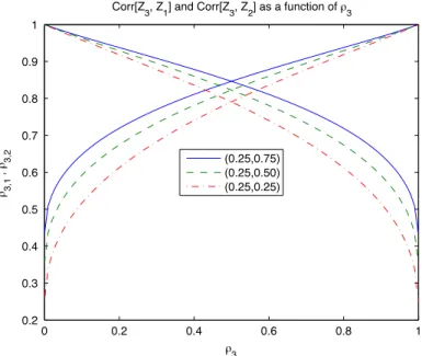
.Fig. 1depicts the above linear correlation coefficients as a function of

ρ3

for several pairs

(ρ1, ρ2)

. It is apparent that Corr

(

Z3,Z1)

=

Corr

(

Z3,Z2)for

ρ3

=

0

.

50, independently of the pair

(ρ1, ρ2)

. Hence,

ρ3

is the dominant driver of the latter correlations.

Now,X

, ξ1, ξ2

i.

∼

i.d.N

(

0

,

1

)

implies that7

(

Z3,Z1)′

∼

N2



µ3

_,1,Σ3,1



,

(47) and

(

Z3,Z1

|

X

=

x

)

′

∼

N2



µ

x 3,1,Σ x 3,1



,

(48) with

µ3

,1

=

(

0

,

0

)

′

;

Σ3,1

=



σ

2 3

ρ3

,1σ3σ1

ρ3

,1σ3σ1

σ

12



;

σ1

=

1

;

7 Since both(Z3,Z1)Tand(Z3,Z1|X=x)Tcan be decomposed asAZ+µ, withZ=(X, ξ1, ξ2)Ta random vector whose components are independent

σ3

=



1

+

2



ρ1ρ2ρ3(

1

−

ρ3)

;

ρ3

,1

=

√

ρ3

+

√

ρ1ρ2(

1

−

ρ3)



1

+

2

√

ρ1ρ2ρ3(

1

−

ρ3)

;

µ

x 3,1

=



√

ρ1ρ3

+



ρ2

(

1

−

ρ3)



x

,

√

ρ1

x

′

;

Σx 3,1

=





σ

x 3

2

ρ

x 3,1σ x 3

σ

x 1

ρ

x 3,1σ x 3

σ

x 1



σ

x 1

2



;

σ

x 1

=



1

−

ρ1

;

σ

x 3

=



ρ3

(

1

−

ρ1)

+

(

1

−

ρ3) (

1

−

ρ2)

;

ρ

x 3,1

=

1



1

+

(1−ρ2)(1−ρ3) ρ3(1−ρ1)

.

By N2

(µ,

_Σ

)

_{we denote the bivariate Normal distribution with mean}

µ

_{and covariance matrixΣ. WriteΦ}2

µ,Σfor the CDF

of the latter, then, from(36), we get

Lt

=

h2(Z3)

=











B[−1]a,b



1

−

Φ 2 µ3,1,Σ3,1



Z3,Hd t



Φ



Hd t





;

−∞ ≤

Z1

<

Htd

;

0

;

H_td

≤

Z1

≤ +∞

.

(49)

Note that the inversez3

=

h[−1]2

(

l

)

, forl

∈

(

0

,

1

]

, can be computed numerically efficiently, thanks to efficient algorithms to compute the bivariate Normal CDF (cf. [20]).

Then, using(39),(40)and(66), it is a trivial task to verify that

Pr



Lt

≤

l





Z₁

≤

H_td

,

X

=

x



=

1

−

Φ2 µx 3,1,Σ x 3,1



h[−1]₂

(

l

),

H_td



Φ



Htd− √ ρ1x √ 1−ρ1



,

(50) Pr [Lt

≤

l

|

X

=

x]

=

1

−

Φ_µ2x 3,1,Σ x 3,1



h[−1]₂

(

l

),

H_td



,

(51) and E



Lt





Z₁

≤

H_td

,

X

=

x



=



1 l=0Φ 2 µx 3,1,Σ3x,1



h[−₂ 1]

(

l

),

Hd t



dl Φ



Htd− √ ρ1x √ 1−ρ1



.

(52)

5.4. Gamma one-factor model

In case of the Gamma one-factor model, to be consistent with the previous section, we suggest to use A(_T3)not

=

.A(_T3)



A(1)

,

A(2)

;

ρ3



=

A(_ρ1) 3T

+

A (2) (1−ρ3)T

,

(53) where A(_ti)not

=

.A(_ti)



Y

, χ

(i)

;

ρ

_i



=

Y_ρ iTt

+

χ

(i) (1−ρi)tT

,

(54) fori

=

1

,

2 andt

∈ [

0

,

T

]

, with

ρ1, ρ2, ρ3

∈ [

0

,

1

]

andY

, χ

(1)

, χ

(2)_{i.i.d. shifted Gamma processes, with shape and} scale parameters chosen such E



A(_ti)



=

0 and Var



A(_ti)



=

t. The latter implies that E



A(_T3)



=

0 and Var



A(_T3)



=

1

+

2 min

{

ρ1ρ3, ρ2

(

1

−

ρ3)

}

.

Finally, notice that(53)can not generally be expressed in the form of(42), due to the fact that the Gamma distribution, and hence the (shifted) Gamma process, do not satisfy the required scaling property. More specifically, recall from(30)that A(_ti)

=

d

µ

_gt

T

−

XAt, withAt

∼

Gamma



α

gTt

, β

g



. From this it is apparent that there will generally exist no functiongsuch thatg

(

c

)

A_t(i)

=

d A(_cti).

The processA(1)_{describes the standardized log-return of the credit, i.e. an obligor defaults ifA}(1)

T

≤

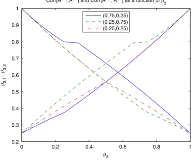
Htd, whereas the processA(2)describes the additional effects influencing the loss rate. The latter two risk factors are dependent, since they

Fig. 2. Pearson correlation betweenA(_T3)andA_T(1),A(_T2).

are both driven by the common processY, as compared to a common factorXin the Normal one-factor model. Note that we actually only need to know the state of the latter process at times

ρ1

(for the default driver) and

ρ1ρ3, ρ2(

1

−

ρ3)

(for the loss driver). Hence, our model can also be regarded as one with 3 mutually correlated systematic risk factorsY_ρ1

,

Y_ρ1ρ3and Y_ρ2(1−ρ3), where the loss rate’s driverA

(3)

T is implicitly related to the former one, by(56), and explicitly related to the latter two, by(53). This is both an advantage as well as an unpleasant side-effect and certainly increases the analytical complexity w.r.t. determining the VaR and DLGD, as mentioned in Section2.1.

Finally, notice thatA(_T3)satisfies(38), where Corr



A(_T3)

,

A(_T1)



=

√

ρ3

+

min

{

ρ1, ρ2

(

1

−

ρ3)

}

1

+

2 min

{

ρ1ρ3, ρ2

(

1

−

ρ3)

}

≥

0

;

Corr



A(_T3)

,

A(_T2)



=

√

(

1

−

ρ3)

+

min

{

ρ1ρ3, ρ2

}

1

+

2 min

{

ρ1ρ3, ρ2

(

1

−

ρ3)

}

≥

0

.

(55)

In line with the third requirement of(38), the above two expressions are bounded from below by Corr

(

Z1,Z2)

=

min

{

ρ1, ρ2

}

. However, contrary to the Normal one-factor model, the above expressions are not symmetric in

ρ1

and

ρ2

.Fig. 2depicts the above linear correlation coefficients, as a function of

ρ3

for several pairs

(ρ1, ρ2)

. Obviously, Corr

(

Z3,Z1)

=

Corr

(

Z3,Z2), for

ρ3

=

0

.

50, only if

ρ1

=

ρ2

. Note also that Corr

(

Z3,Z1), for the pair

(ρ1, ρ2)

, behaves as Corr

(

Z3,Z2), for the pair

(ρ2, ρ1)

. Furthermore, as compared to the Normal one-factor model, in the case of the shifted Gamma model the former correlation coefficient increases much more slowly and the latter correlation coefficient decreases much more quickly as a function of

ρ3

. Hence in the latter model,

ρ3

dominates the dependence less betweenA(_T3)on the one hand andA_T(1)andA(_T2)on the other. Given(53)and(54), and assuming the LGDΛfollows a Beta distribution, the relation between the loss rate and the risk factorA(3)is given by Lt

=

h2



A(_T3)



=















B[−1]a,b





1

−

F A(_T3),A(_T1)



A(_T3)

,

Hd t



1

−

0_αg,βg



µ

_g

−

H_td







;

−∞ ≤

A( 1) T

<

H d t

;

0

;

H_td

≤

A(_T1)

≤

µ

_g

,

(56)

where the joint CDF of the couple



A(_T3)

,

A(_T1)



is generally unknown. Indeed, letGs

∼

Gamma



α

gs

, β

g



, fors

>

0, then it follows from(53)and(54)that

A(_T3)

=

d

µ

_g

−



G_ρ3

+

G1−ρ3



,

which is not necessarily equal in distribution to

µ

g

−

G1, since Corr



G_ρ3

,

G1−ρ3



=

Corr



A(_ρ1₃)_T

,

A(₍2₁₋)_ρ 3)T



=

min

{

√

ρ1ρ3, ρ2

(

1

−

ρ3)

}

ρ3

(

1

−

ρ3)

≥

0

.

Hence, unlike the Normal one-factor model, the distribution of the random variateA(_T3)that drives the loss rate, and thus also of the pair



A(_T3)

,

A(_T1)



, is generally unknown.8Therefore, in order to be able to determine (the inverse of)h2



A(_T3)



we have to numerically estimate the argument

F A(T3),A( 1) T



A(_T3)

,

Hd t



1

−

0_αg,βg



µ

g

−

Htd



=

F_A(3) T   A (1) T ≤Htd



A(_T3)



.

(57)

Once we have constructed the above conditional CDF, it is straightforward to determine the inversea3

=

h[−1]2

(

l

)

, for

l

∈

(

0

,

1

]

.

Finally, lety

(ω)

be a particular realization of the processY, then, Eqs.(39),(40)and(66)lead to

Pr



Lt

≤

l







A (1) T

≤

H d t

,

Y

=

y

(ω)



=

1

−

Pr



A(_T3)

≤

h[−1]₂

(

l

),

A(_T1)

≤

Hd t

|

Y

=

y

(ω)



Pr



A(_T1)

≤

Hd t

|

Y

=

y

(ω)



=

0ϱ1αg,βg[g

(

u1, v1, w1)]

−

0ϱ1αg,βg,ϱ2αg,βg,ρ[g

(

u1, v1, w1) ,g

(

u2, v2, w2)] 1

−

0_ϱ2αg,βg[g

(

u2, v2, w2)]

,

(58) Pr [Lt

≤

l

|

Y

=

y

(ω)

]

=

0ϱ1αg,βg[g

(

u1, v1, w1)]

+

0ϱ2αg,βg[g

(

u2, v2, w2)]

−

0_{ϱ1αg,βg,ϱ2αg,βg,ρ}[g

(

u1, v1, w1) ,g

(

u2, v2, w2)]

,

(59) and E



Lt







A (1) T

≤

H d t

,

Y

=

y

(ω)



=

1

−



1 l=0



0ϱ1αg,βg[g

(

u1, v1, w1)]

−

0ϱ1αg,βg,ϱ2αg,βg,ρ[g

(

u1, v1, w1) ,g

(

u2, v2, w2)]



dl 1

−

0_ϱ2αg,βg[g

(

u2, v2, w2)]

,

(60) with

ϱ1

=

(

1

−

ρ1) ρ3

+

(

1

−

ρ2) (

1

−

ρ3)

∈

(

0

,

1

) ,

ϱ2

=

(

1

−

ρ1)

∈

(

0

,

1

) ,

ρ

=

ρ3



ϱ2

ϱ1

∈

(

0

,

1

) ,

ui

=

ϱ

i

µ

g

,

i

=

1

,

2

,

v1

=

h(₂−1)

(

l

),

v2

=

H_td

,

w1

=

y_ρ1ρ3

+

y_ρ2(1−ρ3)

,

w2

=

y_ρ1

,

g

(

u

, v, w)

=

u

−

v

+

w,

and0m,nthe CDF of a Gamma distribution with shape parameterm

>

0 and scale parametern

>

0 and0m1,n1,m2,n1,ρthe joint CDF of a pair

(

G1,G2), with Corr [G1,G2]

=

ρ

∈

(

0

,

1

)

, whereGifollows a Gamma distribution with shape parameter mi

>

0 and scale parameterni

>

0.

In order to compute the latter bivariate CDF we use five parameter bivariate Gamma CDF in [22], i.e. let Gi

∼

Gamma

(

mi

,

ni

) ,

i

=

1

,

2, with Corr [G1,G2]

=

ρ

≥

0, then, provided thatm1

<

m2,

0m1,n1,m2,n2,ρ[g1,g2]

=

Pr [G1

≤

g1,G2

≤

g2]

,

=

ψ

+∞

−

j=0 +∞

−

k=0 cj,kH



m1

+

k

,

n1g11g1>0 1

−

η



×

H



m2

+

j

+

k

,

n2g21g2>0 1

−

η



;

0

≤

ρ <



m1 m2

,

(61)

8 Though it is possible, in some cases, to determine the CDF of a sum of correlated Gamma random variables. Alouini et al. [21], among others, consider the case of equal shape parameters.

Table 1

Basel II capital charges.

PD Chargeα E [LGD]=10 E [LGD]=60 1 2.10 12.61 5 3.22 19.32 10 4.05 24.28 25 4.94 29.61 with

η

=

ρ



m2 m1

∈

[0

,

1

) ,

ψ

=

(

1

−

η)

m2 0

(

m1)0

(

m2

−

m1)

,

cj,k

=

η

j+k₀

(

_m 2

−

m1

+

j

)

j

!

k

!

0

(

m2

+

j

+

k

)

,

where0

(

·

)

is the Gamma function andH

(

·

,

·

)

is the lower incomplete Gamma function, defined as H

(

a

,

z

)

=

∫

z s=0

sa−1e−sds

.

Note that the requirementm1

<

m2is necessary in order to avoid the poles 0

,

−

1

,

−

2

, . . .

of the Gamma function in computing

ψ

andcj,k. The limit case wherem1

=

m2

=

m, which occurs if

ρ1

=

ρ2

or

ρ3

=

1, can be dealt with using the four parameter bivariate Gamma CDF in [22], i.e.,

0m,n1,m,n2,ρ[g1,g2]

=

ψ



+∞

−

k=0



ckH



m

+

k

,

n1g11g1>0 1

−

ρ



H



m

+

k

,

n2g21g2>0 1

−

ρ



;

0

≤

ρ <

1

,

(62) with



ψ

=

(

1

−

ρ)

m 0

(

m

)

,



ck

=

ρ

k k

!

0

(

m

+

k

)

.

Finally, it is left as an exercise to the reader to verify that the association parameter

η

=

ρ3

, if

ϱ1

> ϱ2

(or equivalently

ρ1

> ρ2

) and that

η

=

ρ3

ϱ2

ϱ1

=

1 1+(1−ρ2)(1−ρ3)

ρ3(1−ρ1)

, if

ϱ1

≤

ϱ2

. Hence, by construction, we always have

η

∈

(

0

,

1

)

. Note that the boundary cases

ρ3

=

1 or

ρ2

=

1 imply

η

=

1, whereas

ρ3

=

0 or

ρ1

=

1 imply

η

=

0.

6. Numerical results

In this section we implement stochastic recovery in the Normal factor model and the (shifted) Gamma one-factor model. In a first, Basel II-oriented, experiment, we will examine the sensitivity of the required capital charge, i.e. VaR_α

(

Lt

)

−

E [L], and the DLGD, at level

α

=

99

.

99%, to changes in the expected value of the LGD (assumed to be Beta

(

a

,

b

)

distributed), the PD and the correlation coefficients

ρ

i

,

i

=

1

,

2

,

3. In a second, CDO base-correlation curve-oriented, experiment we will compare the relation between the CLGD and the systematic factor induced by our framework to the corresponding LGD

(

C

)

-curves according to Amraoui and Hitier [14] and Andersen and Sidenius [10].

6.1. Basel II: sensitivity analysis

In this