Evaluation of Support Vector Machine kernels for detecting network anomalies

(1)

Evaluation

of

Support

Vector

Machine

Kernels

for

Detecting

Network

Anomalies

by

Prerna

Batta

B.Tech,LovelyProfessionalUniversity,2013

ThesisSubmittedinPartialFulfillmentofthe RequirementsfortheDegreeof

MasterofAppliedScience

inthe

SchoolofEngineeringScience

FacultyofAppliedScience(EngineeringScience)

©PrernaBatta2019 SIMONFRASERUNIVERSITY

Summer2019

Copyrightinthisworkrestswiththeauthor.Pleaseensurethatanyreproductionorre-use isdoneinaccordancewiththerelevantnationalcopyrightlegislation.

(2)

Approval

Name: Prerna Batta

Degree: Master of Applied Science

Title: Evaluation of Support Vector Machine Kernels for Detecting Network Anomalies

Examining Committee: Chair: Ivan V. Baji´c

Professor Ljiljana Trajkovi´c Senior Supervisor Professor Parvaneh Saeedi Supervisor Associate Professor

Mirza Faisal Beg

Internal Examiner Professor

(3)

Abstract

Border Gateway Protocol (BGP) is used to exchange routing information across the Internet. BGP anomalies severely affect network performance and, hence, algorithms for anomaly detection are important for improving BGP convergence. Efficient and effective anomaly detection mechanisms rely on employing machine learning techniques. Support Vector Machine (SVM) is a widely used machine learning algorithm. It employs a set of mathematical functions called kernels that transform the input data into a higher dimensional space before classifying the data points into distinct clus-ters. In this Thesis, we evaluate the performance of linear, polynomial, quadratic, cubic, Gaussian radial basis function, and sigmoid SVM kernels used for classifying power outage such as Moscow Power Blackout, BGP mis-configuration, and BGP anomalies such as Slammer, Nimda and Code Red I. The SVM kernels are compared based on accuracy and the F-Score when detecting anoma-lous events in the Internet traffic traces. Simulation results indicate that the performance heavily depends on the selected features and their combinations.

Keywords:Border gateway protocol; routing anomalies; machine learning; feature selection; sup-port vector machine; kernels.

(4)

Dedication

(5)

Acknowledgements

I express my gratitude to my senior supervisor Prof. Ljiljana Trajkovi´c for her guidance and count-less hours spent for reviewing my work. She has always been very encouraging and supportive. She always allowed me to explore my ideas and I am very thankful to her for the time and efforts she invested in me and my research work. This would not have been possible without her hard work and support.

I would also like to thank my committee chair Ivan V. Baji´c and committee members Prof. Parvaneh Saeedi and Prof. Faisal Beg for providing valuable comments and suggestions.

I am very thankful to my colleagues in the Communication Networks Laboratory. Special thanks to Zhida Li for his friendship and support during my graduate studies. I also thank Dr. Maninder Singh, Qingye Ding, and Ana Gonzalez for their valuable comments and suggestions.

My deepest gratitude goes to my family for their support and unconditional love. I am very thankful to my mother Swati Batta and father Rajeev Batta for always advising me to work hard and pursue my studies. You both are my guiding light and my pillar of strength. Thank you for believing in me. Last but not least, I would also like to extend my gratitude to my friends Anmit Deol, Jaspreet Gill, and Gursimran Sahota who have provided support in countless ways and always motivated me to keep working hard to achieve my goals. I am very grateful to my brother Ankit Batta. You supported me through the toughest times of my life. Without you, I would not have made it this far.

(6)

List of Tables

Table 3.1 Behaviour of sigmoid kernel . . . 24

Table 4.1 List of BGP attributes . . . 27

Table 4.2 List of features extracted from BGP update messages . . . 27

Table 4.3 Details of the anomalous events . . . 28

Table 5.1 Confusion matrix . . . 37

Table 5.2 Area under curve for the six types of SVM kernels used . . . 39

Table 5.3 Training and test datasets . . . 40

Table 5.4 Accuracy and F-Score using SVM with Linear kernel . . . 41

Table 5.5 Accuracy and F-Score using SVM with Polynomial kernel . . . 42

Table 5.6 Accuracy and F-Score using SVM with Quadratic kernel . . . 43

Table 5.7 Accuracy and F-Score using SVM with Cubic kernel . . . 44

Table 5.8 Accuracy and F-Score using SVM with Gaussian kernel . . . 45

(9)

List of Figures

Figure 2.1 Support Vector Machine. . . 5 Figure 2.2 Selection of hyperplanes in a two-dimensional feature space. . . 6 Figure 2.3 Decision surface and the margin. . . 7 Figure 2.4 Selection of a hyperplane in n-dimensional feature space, whereφ

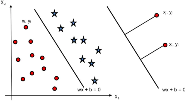
repre-sents mapping . . . 8 Figure 2.5 Illustration of arbitrary point (xi, xj) lying on one side of the decision

sur-facewx+b=0(left) and the functional margin (right). . . 10 Figure 2.6 Geometric margin: SVM maximizes the geometric margin by learning a

suitable decision surface. . . 11 Figure 2.7 Illustration of normalized SVM formulation. . . 13 Figure 2.8 Illustration of SVM with noise margin. . . 14

Figure 3.1 Illustration of SVM using the nonlinear kernel functionk(x1,x2) =hx1,x2i2.

View in the three-dimensional space shows a hyperplane dividing regular (circles) and anomalous (stars) data points. . . 17 Figure 3.2 Illustration of SVM with linear kernel: Shown are correctly classified

reg-ular (circles) and anomalous (stars) data points as well as one incorrectly classified regular (circle) data point. . . 19 Figure 3.3 Polynomial kernels forp=1(top) andp=2(bottom). . . 21 Figure 3.4 Gaussian kernels forσ = 20(left) andσ= 1(right). . . 23

Figure 4.1 Number of BGP announcements between January 23, 2003 and January 28, 2003. The announcements occurred during the Slammer worm attack are labelled as the "anomaly" class while others are labelled as the "regu-lar" class. . . 29 Figure 4.2 Number of BGP announcements between September 16, 2001 and

Septem-ber 21, 2001. The announcements occurred during the Nimda worm attack are labelled as the "anomaly" class while others are labelled as the "regu-lar" class. . . 29

(10)

Figure 4.3 Number of BGP announcements between July 17, 2001 and July 22, 2001. The announcements occurred during the Code Red I (version 2) worm at-tack are labelled as the "anomaly" class while others are labelled as the "regular" class. . . 30 Figure 4.4 Number of BGP announcements between December 18, 2001 and

Decem-ber 22, 2001. The announcements occurred during regular RIPE traffic be-long to the "regular" class. . . 30 Figure 4.5 BGP announcements during Slammer: maximum AS-path length (top left),

maximum AS-path edit distance (top right), number of EGP packets (bot-tom left), and number of duplicate announcements (bot(bot-tom right) [13]. . . 31 Figure 4.6 Distribution of maximum AS-path length (top) and maximum AS-path edit

distance (bottom) collected during the Slammer worm attack [13]. . . 32 Figure 4.7 Distribution of number of BGP announcements (top) and withdrawals

(bot-tom) for the Code Red I (version 2) worm attack [13]. . . 33 Figure 4.8 Scattered graph of Feature 9 vs. Feature 6 (top) and Feature 1 (bottom)

extracted from the BCNET traffic [13]. . . 35

Figure 5.1 ROC curve for the kernels with highest AUC i.e. Linear 0.96, Polynomial 0.94, and Gaussian RBF 0.93. . . 39

(11)

Chapter 1

Introduction

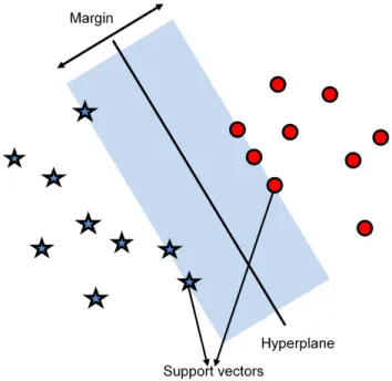
Machine learning is a subset of artificial intelligence that deals with designing algorithms, building models and making decisions based on the input datasets. Machine learning models classify data using a feature matrix. The rows and columns of the matrix correspond to data points and feature values, respectively. By providing a sufficient number of relevant features, machine learning algo-rithms help build models to more accurately classify data. They have been recently used to optimally solve a variety of engineering and scientific problems. Among various machine learning approaches such as Logistic Regression, naïve Bayes, and Support Vector Machine (SVM), SVM is often used due to its robust nature [1]. It classifies data by defining a decision boundary to lie geometrically midway between the support vectors. Support vectors are the data points that lie closest to the de-cision surface. SVM deals with both linearly and nonlinearly separable features of the input dataset by using kernels.

Machine learning algorithms are classified as supervised and unsupervised learning. Kernel functions are used to map a nonlinearly separable into a higher-dimensional linearly separable data [2].

1.1

Supervised Learning

The term "supervised learning" refers to algorithms that learn from training dataset and are being trained to supervise the learning process. The algorithm learns the mapping function to derive an output from the given input. The learned mapping function is then used to predict the output for new input data. After multiple iterations, the algorithm achieves a desirable level of performance for predicting the outcomes. Classes used in supervised learning are known which implies that all input data is labelled. The goal of supervised learning is to identify clusters of data. Supervised learning is typically used when we wish to perform classification (map input labels to output labels) or regression (map input labels to a continuous output labels). Supervised learning is used to train a model to perform regression or classification. Hence, supervised learning algorithms are classified into classification and regression groups:

(12)

• Classification: The output variable falls into a category. Example: "This apple is green in colour" or "this apple is red in colour".

• Regression: The output variable has a numerical value. Example: "The height of this building is 100 feet" or "Frank only has 100 dollars in his account".

In both cases, the goal is to find specific connection or structure among the input variables that would help produce the correct output. The output is determined based on the training data. The supervised learning produces accurate and reliable results because the input variables are known and labeled, which implies that the algorithm will only attempt to identify the hidden patterns.

1.2

Unsupervised Learning

In "unsupervised machine" learning, the input data is uncategorized (unlabeled). Unlike supervised learning, there is no prior knowledge of the data and the number of classes are not known. Without knowing the labels, unsupervised learning algorithm models the distribution of the input data [3]. The algorithm has to define and label the input data before determining the hidden patterns and structure. It is expected to group the data into clusters using various categories. These algorithms are grouped into clustering and association groups:

• Clustering: Find inherent groupings within the input data. Example: grouping customers by their social status.

• Association: Find various associations between different groups of input data. Example: cus-tomers that buy item A tend to buy item B as well.

Clustering is the most common unsupervised technique used to find the hidden patterns or create clusters. Unsupervised learning is used to explore the data and train a model to spilt data up into clusters. The most common algorithm used for performing clustering is k-means.

1.3

Support Vector Machine

SVM is a supervised machine learning algorithm that takes a known set of data as an input. It builds a model for the known input. Based on the model, it predicts the outcome [4] for new data. There are two main stages in supervised learning: training and testing. In the training stage, the supervised algorithm builds the model while in the testing phase, the same model predicts the output. SVM is the most robust Machine Learning algorithm designed by Cortes and Vapnik [4].

SVM considers each feature as a point in n-dimensional space and classifies the data into two classes by using a hyperplane. For example, for a two-dimensional space, the hyperplane is a line. In higher dimensions (3 and higher), the separation is a hyperplane. The goal of SVM is to find maximum separation between two classes. Data points that lie on the edge of the plane are called support vectors. Two basic rules that govern the selection are:

(13)

• Step 1: Select the hyperplane that separates the data into two distinct classes.

• Step 2: Maximize the distance between the nearest data points of either class such that no data point is misclassified.

Support Vector Machine (SVM) was originally formulated to address binary classification prob-lems. It was used as a method in extending logistic regression to generate maximum entropy classi-fication models. The general formulation of SVM [5] includes:

• Linear learning function as the classification or the regression model;

• Constraints defining the theoretical bounds;

• Convex duality and formulations concerning the associated dual-kernel;

• Dual-kernel formulations sparseness.

The combination of these processes makes SVM robust and unique. SVM offers a clear computa-tional advantage over the standard statistical methods.

1.4

Research Contributions

In this Thesis, we have revised and extended our previous research findings and results [10–16] by employing various SVM kernels for detecting BGP anomalies. We consider BGP update mes-sages that are extracted from the data collected during the time periods when the Internet experi-ences known anomalies. The performance of anomaly classifiers is closely related to the selected features. Past approaches to select BGP feature employed minimum Redundancy Maximum Rele-vance (mRMR) [6] algorithms such as Mutual Information Deference (MID), Mutual Information Quotient (MIQ), and Mutual Information Base (MIBASE). In this Thesis, we employ the decision tree algorithm for feature selection and evaluate performance of SVM using linear, quadratic, cubic, polynomial, Gaussian RBF, and sigmoid kernels.

For experiments, we use a Windows 10 64-bit PC with 16 GB RAM and Intel Core i5 processor. We perform experiments in Matlab R2019a [27] with Statistics and Machine Learning Toolbox to evaluate the performance of SVM kernels. All kernel functions are in-built in the Classification Learner application of the Matlab tool. We select 37 features or the most relevant features using the decision tree algorithm. Some features are removed from the constructed decision tree because they are repeatedly used [12]. We train the SVM with linear, polynomial, quadratic, cubic, Gaussian RBF, and sigmoid kernels. We test the models using various datasets and evaluate the performance of the SVM kernels based on accuracy and F-Score. The performance of SVM using linear, quadratic, and cubic kernels has been reported in [10]. In this Thesis, we have extended our work by adding the performance of SVM using polynomial, Gaussian RBF, and sigmoid kernels.

(14)

1.5

Organization of the Thesis

The Thesis is organized as follows: We first briefly describe supervised learning, unsupervised learn-ing, and SVM algorithms. We provide an overview of the SVM algorithm as well as the description of hyperplane and margins in Chapter 2. In Chapter 3, we describe SVM with kernels including linear and various types of nonlinear kernels. BGP datasets used for detecting network anomalies, BGP anomalies that have been considered in this Thesis, and feature selection is given in Chapter 4. We compare the performance of SVM using linear and nonlinear kernels in Chapter 5 and conclude with Chapter 6. The list of references is provided in the Bibliography section.

(15)

Chapter 2

Support Vector Machine Algorithm

Support Vector Machine (SVM) is one of the most effective classifiers. It handles linear as well as nonlinear functions using various kernels. SVM may be used with datasets having larger number of features without adding too much complexity to the system [34]. SVM tries to classify the given data points into two groups as shown in Fig. 2.1.

Figure 2.1: Support Vector Machine.

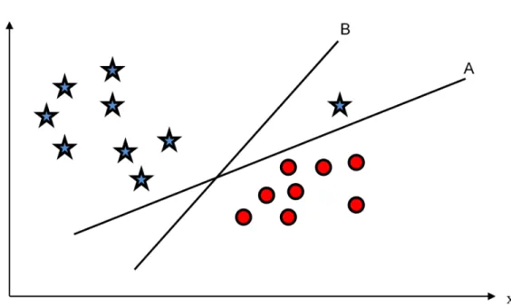
By selecting hyperplane B one data point is misclassified. Fig. 2.2 shows that hyperplane A is best suited for classifying the given data.

(16)

Figure 2.2: Selection of hyperplanes in a two-dimensional feature space.

Consider the case of logistic regression where we consider the output of the linear function and find the value within the range of 0 and 1 by using the logistic sigmoid function, which is an s-shaped curve that takes any real number and maps it into a value between 0 and 1. Typically, label 1 is used if the value is greater than a threshold value. Otherwise, label 0 is assigned. If xandy are the input and output variables, respectively, logistic regression tries to find the probability that y= 1given the inputx:

P(y=1 |x). (2.1)

We use the logistic sigmoid function to map predicted values to probabilities:

h(x) = 1

1 +e−x, (2.2)

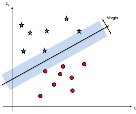
whereh(x)is the output between0and1,xis the input to the function, andeis the base of natural log. The model attempts to maximize the distance between the training instance and the decision surface. A surface in a multidimensional state space that divides the space into different regions is called decision surface. Data points lying on side of a decision surface belong to a different class from those lying on the other side of a decision surface. The distance between the closest point and the decision surface is called a margin, as shown in Fig. 2.3.

(17)

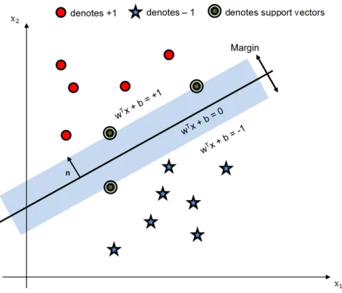
Figure 2.3: Decision surface and the margin.

Among all decision surfaces, the surface that gives maximum margin is selected. The points ly-ing closest to the decision surface are called support vectors. For a linearly separable two-dimensional feature space, there are at least two support vectors. These support vectors determine the decision surface [35]. Various SVM kernels may be employed for classification. If a dataset is not linearly separable, SVM with linear kernel performs poorly [28]. In such a scenario, polynomial nonlinear SVM kernels are used. Nonlinear kernels enlarge the feature space of input datasets to generate non-linear boundary between the classes. This is achieved by mapping the data to a higher dimensional space. Such a boundary created by nonlinear kernels appears as a linear hyperplane and is used to extend SVM to nonlinear surfaces.

2.1

Nonlinear Hyperplane

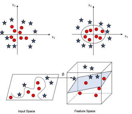
For a two-dimensional dataset, it is relatively easy to find a hyperplane. In such cases, kernels are used to generate the hyperplanes. Kernels are the mathematical functions used to transform two-dimensional points into n-dimensional space [33]. It is a type of data transformation function. Once the data points are transformed into n-dimensional space, a hyperplane is then built so that it separates the data into distinct sets. As shown in Fig. 2.4, the kernel function used to generate the hyperplane is of the formx2+y2 =z2. The corresponding hyperplane is a circle that separates the two data points without misclassifications.

(18)

Figure 2.4: Selection of a hyperplane in n-dimensional feature space, whereφrepresents mapping

The objective function for SVM with nonlinear kernel has the form [1]:

max X i λi− 1 2 X i X j λiλjyiyjxi·xj, (2.3)

whereλiandλj correspond to the points that are closest to the margin. The objective function (2.3)

depends on the dot product of input vector pairsxi ·xj that represents a kernel function. Standard

machine learning methods may be formulated as the task of minimizing a convex function f that depends on a variable vector w with nentries. This can be formally written as the optimization problem:

minw∈Rnf(w), (2.4)

wheref(w)is the objective function of the form:

f(w) =λR(w) + 1 n i=1 X n L(w;xi, yi), (2.5)

wherexi ∈ Rnare the training data for1 ≤ i ≤ nandyi ∈ Rare their corresponding labels

that we wish to predict. In any classification problem, the objective function may be defined as a sum of regularization and loss functions. The objective functionf has two parts: the regularization function that controls the complexity of the model and the loss function that measures the error of the model using the training data. The loss function L(w;x, y) is a convex function ofw. The

(19)

regularization parameterλ ≥ 0defines the trade-off between minimizing the loss (training error) and the model complexity (overfitting).

Let xi be the input sample, yi the output label,wthe weight vector, and λthe regularization

parameter. The objective function may be written as:

minwλ||w||2+

n

X

i=1

(1−yi[xi,w]). (2.6)

A loss function indicates the quality of the employed classifier. The smaller the loss function, the better is the classifier at classifying the input data. The amount of work required in order to increase the classification accuracy is proportional to the loss function. The input vector isxi, the

output label isyi, and the weight vector wneeds to be calculated. Hence, the objective function

calculates weight so that the system trains and builds its model. Therefore, the loss function in (2.5) is the dot product of the output vector and input samplesxi. The sum:

n

X

i=1

(1−yi[xi,w]). (2.7)

gives the total loss over the entire set of sample points. Minimizing the objective function leads to the minimum loss.

2.2

Functional Margin

Consider an arbitrary point (xi, yi) lying on one side of the decision surface. Suppose that the

equa-tion of the decision surface is given by:

wx+b= 0, (2.8)

wherewis a weight vector,xis the input vector, andbis the bias. Letx1andx2be the two features.

The equation of the decision surface may be written as:

x1w+x2w+b= 0. (2.9)

Consider the point (xi, yi)with respect to the line (w, b). The functional margin is a distance

between(xi, yi)and the decision boundary(w, b). To find this distance, consider the straight line

(20)

Figure 2.5: Illustration of arbitrary point (xi, xj) lying on one side of the decision surfacewx+b=

0(left) and the functional margin (right).

Let a vector (w1,w2)lie perpendicularly to this line. The distance of(xi, yi)from the decision

surfaceγiis given by:

γi =yi(wTxi+b), (2.10)

wherewT is the optimal weight vector, (xi, yi) are arbitrary points, andbis the bias. An arbitrary

point (xj, yj) will have a different functional margin. As shown in Fig. 2.5, the functional margin

for (xj, yj) is larger than the functional margin for (xi, yi), which implies that if the point is further

away from the decision surface, there is higher confidence in its classification. Therefore, larger functional margin implies better confidence in predicting the class of an arbitrary point. Weight vectorwT and biasb may be arbitrarily scaled (2.10). Even though the slope remains the same, the functional distance increases or decreases depending onwT andb. Hence, functional margin is seldom used as the most important SVM parameter [40]. For example, for multiple training data pointsS = (x1, y1),(x2, y2), ...,(xi, yi), the functional marginγis given as:

γ =minn

i=1 γ

i_. _(2.11)

A geometrical margin is invariant to the scaling as shown in Fig. 2.5. Any line to the decision surfacewx+b = 0isw. Hence, the unit vector perpendicular to the decision surface is given by

w

||w||. As an example, consider the line given by2x+ 3y+ 1 = 0. Hence,w= (2,3) and ||ww||:

w ||w|| = 2 √ 13, 3 √ 13 . (2.12)

(21)

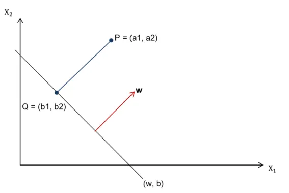
Now consider a point P with coordinates (a1, a2), as shown in Fig. 2.6. Geometric margin of a

hyperplane is defined as functional margin scaled byw.

Figure 2.6: Geometric margin: SVM maximizes the geometric margin by learning a suitable deci-sion surface.

A perpendicular line from a pointP to the decision surface connects at a pointQwith coordi-nates (b1, b2). The smallest distance betweenP andQis in the direction of the perpendicular vector.

Hence: P = Q +γ w ||w|| (a1, a2) = (b1, b2) +γ w ||w||, (2.13)

whereγ is the decision surface. Solving forγgives:

wT(a1, a2)−γ w ||w|| +b= 0. (2.14) Hence, γ = w T₍_a 1, a2) +b ||w|| = w T ||w||(a1, a2) + b ||w|| =y w T ||w||(a1, a2) + b ||w|| ∀ y=±1, (2.15)

(22)

wherewis scaled so that||w||= 1. The geometric margin after normalization is:

γ =ywT(a1, a2) +b

. (2.16)

For a given set of points, the geometric margin is the smallest of all margins for the individual points. Hence,

γ =minn

i=1 γ

i_. _(2.17)

We have assumed that the data points are linearly separable. The selected classifier should have maximum margin width and be robust to the outliers. Such a classifier will have a strong general-ization ability to separate all the data points into two distinct classes. The geometric marginγ||w||

needs to be maximized subject to certain constraints. Hence, the optimization problem reduces to:

maximize γ

||w||

subject to yi(wTxi+b)≥γ, i= 1,2, ..., N,

(2.18)

where N is the size of training data.

If (w, b) characterizes the decision surface,γ/||w||is the geometric margin. SVM learns the values of(w, b)so that the geometric mean is the largest subject to the following constraints:

yi(wxi+b)≥γ, for positive data points

yi(wxi+b)≤γ, for negative data points.

(2.19)

In order to normalize the function,wis scaled so that the geometric margin is1/||w||= 1, as shown in Fig. 2.7. Transforming the problem into minimization, normalized SVM may be formulated as:

minimize 1

2||w||,

such that yi(wTxi+b)≥1.

(23)

Figure 2.7: Illustration of normalized SVM formulation.

Hence, SVM is a quadratic optimization problem with convex quadratic objective and a set of linear inequality constraints. It may be solved using quadratic programming solvers.

2.3

Maximum Margin With Noise

When data is not linearly separable, linear SVM mathematical formulations fails to perform. To deal with the nonlinear separability of data points, changes are made to the objective function. Along with maximizing the margin, objective function should also incorporate a function to minimize the number of misclassifications, as shown in Fig. 2.8.

(24)

Figure 2.8: Illustration of SVM with noise margin.

The objective function may be written as:

minimize: ||w||+ C·training errors, (2.21)

whereCis the control parameter. Letf(ξn)be the penalty function associated with each

misclassi-fied training point. Minimizing the penalty function reduces the number of misclassimisclassi-fied instances. Hence, the problem may be formulated as:

minimize ||w||+ C· N X n=1 f(ξn), with constraints yn(w·xn+b)≥1−ξn ξn≥0, (2.22)

where N is the size of training data.

Slack variables ξn are used to calculate the training errors by measuring the distance of each

training data point to its marginal hyperplane. By adding the slack variables (ξs, ξ2, ..., ξn) to the

penalty function, the objective function reduces to a minimization problem. The constraint (yn(wxn+

b) ≥ 1) will no longer be true for misclassified points. Hence, penalty function is remodeled to yn(w·xn+b)≥(1−ξn ∀ n= 1,2, ..., N). In order to convert a constrained optimization

(25)

multipliers may be written as: L(w, b, ξ, α, β) = 1 2||w||+ C· N X n=1 ξn + N X n=1 αi[yn(x·w+b)−1 +ξn]− N X n=1 βnξn, (2.23)

whereC is a trade-off parameter to balance the violation of the margin whileαnandβn are the

Lagrange multipliers≥0. Given these Lagrangian multipliers, the dual formulation is:

maxα(α) = N X n=1 αn− 1 2 N X n=1 αnyn(xTn). (2.24)

In case of SVM without noise:

αin≥0, n= 1, ..., N N X n=1 αnyn= 0. (2.25)

In case of SVM with noise:

0≤αn≤C, n= 1, ..., N N X n=1 αnyn= 0. (2.26)

In a dual formulation, the objective function remains the same while the constraints vary depending whether or not the noise factor is taken into account. If there is noise, the SVM valueαn∈[0, C].

The SVM classifier with noise is commonly called assoft SVM because it lacks a hard decision boundary that separates the different classes of data points. The soft margin classification is de-fined as identifying support vectors. Data pointsxn that have non-zero corresponding Lagrangian

multipliersαnserve as the support vectors. The solution to the dual problem is:

w= N X i=n αnynxn b=yn(1−ξn)− N X n=1 αnynxn. (2.27)

Solution to a classification problem may be formulated as:

f(x) =

N

X

n=1

αnynxnx+b, (2.28)

wherexis the test point,ncorresponds to those points whereαn6= 0are the support vectors, andb

(26)

Chapter 3

Using SVM with Kernels

The kernel function defines inner productshxn, xmi. Letφ(x)be a mapping of feature vectors from

an input space to a feature space:

hxn,xmi → hφ(xn), φ(xm)i. (3.1)

The input space represents the selected features from the original dataset while the feature space is generated by the mappingφ(x). An example of mappingφ(x) : R2 → R3 is shown in Fig. 3.1, where:

(xi, xj)→(x2i,

√

2xixj, x2j). (3.2)

Ifx(x1, x2)andx0(x01, x02)are two feature vectors (data points) in the input space, then:

hφ(x1, x2), φ(x01, x02)i= h(x12, √ 2x1x2, x22),(x01 2 ,√2x0₁x0₂, x02₂)i= (x1x01+x2x02)2= (hx, x0i)2 =k(x, x0), (3.3)

wherek is a kernel function. Instead of calculating eachφ(x), the “kernel trick" is introduced to directly calculate the inner product in the input space:

k(xn,xm) =hφ(xn), φ(xm)i. (3.4)

The mapping (3.4) defines the feature space and generates a decision boundary for input data points. Using the “kernel trick” reduces the complexity of the optimization problem that now only depends on the input space instead of the feature space [39]. If the dataset is nonlinearly separable, the original feature space or the input featuresxare transformed into a new feature spaceφ(x). The training data points are usually mapped to high dimensional feature space to make them linearly separable. The computational costs for such a transformation are very high [41]. For input feature space havingDdimensions, the computational time required isO(D2)and the computational cost increases with dimensionD. Using kernel functions achieves the transformation without increasing the computational cost.

(27)

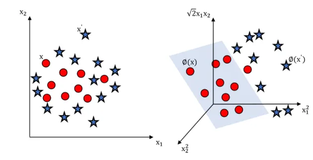
As shown in Fig. 3.1, the graph on the left-hand side shows two attributes(x1,x2), the regular

data points (circles) lie inside while the anomalous data points (stars) lie outside. No line can be drawn to separate them into two distinct classes. However, if the same set of data points are trans-formed into another feature space having two dimensions (x2₁,x2₂), the regular data points (circles) and anomalous data points (stars) become linearly separable, as shown on the right-hand side of Fig. 3.1.

Figure 3.1: Illustration of SVM using the nonlinear kernel function k(x1,x2) = hx1,x2i2. View

in the three-dimensional space shows a hyperplane dividing regular (circles) and anomalous (stars) data points.

Suppose that x and x0are original features that are transformed toφ(x)andφ(x0), respectively. To solve SVM in this new feature space, the scalar productφ(x) · φ(x0) is required. For certain functions (φ), there is a simple operation on two vectors in the lower dimensional space that may be used to compute the scalar product of their two mappings in the higher dimensional space:

φ(x) · φ(x0) =k(x,x0). (3.5)

There is no need to individually solve or expand the originalφ(x)andφ(x0). Functions such asφ are called kernel functions. The following steps solve SVM using kernel functions:

• Step 1: Original input attributes are mapped to a new set of input features via feature mapping φ.

• Step 2: The algorithm may be now applied using the scalar product: replace x · x0 withφ

(x) · φ(x0).

(28)

dimensional space:

k(x,x0) =φ(x) · φ(x0). (3.6)

The scalar product in the high dimensional space ensures the lower computational costs. Using the feature mapping, the discriminant function may be written as:

g(x) =wTφ(x) +b= X

i∈SV

αiφ(xi)Tφ(x) +b, (3.7)

whereiranges over the support vectors (SV). Consider 2-dimensional vectorxhaving two attributes (x1, x2). The kernel function may be written as:

k(x1,x2) = (1 +x1,x2)2 = 1 +x2₁x2₂+ 2x1x2x01x 0 2+x21 0 x2₂0+ 2x1x1+ 2x01x 0 2 = (x2₁ √ 2x1x01x21 0√ 2x1 √ 2x0₁)·(x2₂ √ 2x2x02x22 0√ 2x2 √ 2x0₂) =φ(x1)φ(x2), (3.8) whereφ(x)= x2₁√2x1x2x22 √ 2x1 √

2x2. Hence, by using the transformationφ, the kernel function

may be easily computed without expanding the scalar product. Kernel function may be considered as a similarity measure between the input objects. However, not all similarity measures may be used as kernel functions. Only similarity functions that satisfy the Mercer’s condition qualify as kernel functions [31]. Mercer’s condition states: If similarities between the points are written as a matrix and this matrix is symmetric positive semi-definite, than a kernel function exists. For any positive semi-definite kernelk(x1,x2), satisfying:

X

1,2

k(x1,x2)c1c2 ≥0. (3.9)

k(x1,x2)may be considered as kernel function for any real value of c1and c2because such functions

may be expressed as a dot product in high dimensional space. Some commonly used kernel functions are linear, polynomial, quadratic, cubic, Gaussian radial-basis function, and sigmoid. The choice of the kernel depends on the type of input data. For example, Gaussian kernel defines a function space that is much larger than the function space defined by the linear or polynomial kernels. Linear and polynomial kernels have limited complexity and fixed size. Hence, the SVM model using linear or polynomial kernel converges much faster. Gaussian kernel belongs to the category of nonlinear kernels and its complexity increases with the size of input data. However, it is more flexible than the linear and polynomial kernels.

For a given dataset, there exists a hyperplane that correctly classifies the data points into distinct classes. Indeed, in most cases there is a number of such hyperplanes. With many choices, there is al-ways a question of the best selection of the hyperplane. The necessary condition is to ensure correct classification of the training data. The classifier still has to be applied to the test data. Intuitively, the

(29)

classifier should be tested using all the kernels functions and, as per statistical learning theory [39], that kernel function should finally be used as a hyperplane classifier that provides the maximum margin between various attributes.

3.1

Linear Kernel

Linear SVM corresponds to linear kernel where φ(x) = x and φ(x0) = x0. Often used for text classification, the linear kernel optimization problem is much faster compared to others [31]. It is typically used when the number of features is large and nonlinear mapping fails to improve the performance due to large feature space. As shown in Fig. 3.2, decision boundary separates both correctly and incorrectly classified data points.

Figure 3.2: Illustration of SVM with linear kernel: Shown are correctly classified regular (circles) and anomalous (stars) data points as well as one incorrectly classified regular (circle) data point.

Finding a suitable class for thousands of training data is often very time consuming. To reduce the running time, two tuning parameters (regularization parameter and gamma) are introduced in SVM classifiers. By fine tuning the two tuning parameters, nonlinear classification may be achieved within reasonable time. Regularization parameter sets the limit on the number of misclassifications that may be tolerated for each training example. For higher values of the regularization parameter, the optimizer will choose a small margin hyperplane. The gamma parameter defines the influence a given training example exerts: smaller values imply higher influence while larger values imply smaller influence.

3.2

Nonlinear SVM Kernels

Soft SVM enabled accounting for the noise and finding the classifiers that do not precisely separate different sets of data points. However, the classification decision surface is still linear and cannot handle cases where the decision surface is nonlinear. To develop an input-output functional relation-ship, the easiest and straightforward approach is to consider the output variable as a linear combina-tion of its input vector components [32]. The linear combinacombina-tion may use the least square methods for regression and classification problems. Although simple, linear models have limited

(30)

classifica-tion power. Nonlinear models give more enhanced predicted outputs. However, these models have two significant problems:

• It is rather difficult to analyze nonlinear models.

• They require large computational infrastructure to achieve a satisfactory solution.

The optimal solution for a linear-nonlinear dilemma is to utilize advantageous features of both models. Instead of using only nonlinear models, problems are modeled so that the linear character of the problem remains intact while and the features are modified to increase the classification power of the linear methods. Nonlinear function feature components are transformed using various kernels so that nonlinear functional relationship may be considered as a linear function.

3.2.1 Polynomial Kernel

Polynomial kernel employs polynomial function to the input variables to find the similarity in train-ing vectors. These types of nonlinear kernels are extensively used for problems where traintrain-ing data is normalized. Its generalized form is defined as:

K(xi,xj) = (1 + xi,xj)p, (3.10)

wherepis the degree of the polynomial. For example,p = 2andp = 3for a quadratic and cubic kernels, respectively. A polynomial kernel is often used for visual pattern recognition and natural language processing classifications.

A degree of the polynomial kernel governs the flexibility of the resulting classifier. Forp= 1, the classifier has a linear kernel that is not sufficient to occupy the nonlinear feature space. The function space of the problem increases with the degree of polynomial. Polynomial kernels with degrees 1 and 2 are shown in Fig. 3.3.

(31)

Figure 3.3: Polynomial kernels forp=1(top) andp=2(bottom).

For apthorder polynomial kernel, all derivatives of orderp+ 1are constant and, subsequently, all derivatives of orderp+ 1and higher are zero.

(32)

3.2.1.1 Quadratic Kernel

Each type of classifier and the kernel generates a distinct decision boundary. For example, the decision boundary generated using quadratic kernel is quite different from the shape of a simple quadratic function in 2-dimensional space. Using the quadratic kernel, one may visualize the given data points being lifted to fit into the shape of a quadratic function and forming a shape of the ellipse if cut by the plane. Suppose there are only two features (x1, x2). Quadratic kernel expands the two

features into five (x1, x2, x21, x22, x1x2). The decision boundary in such a case may be given by:

wTφ(x) +b= 0, (3.11)

wherewT is a vector, b is bias, andφ(x) = (x1, x2, x21, x1, x2, x22).

Quadratic kernel leads to decision boundary containing a mixture of quadratic functions. The decision boundary is defined asy|P

iαik(xi, y) =b. For example, consider the decision boundary

and the kernel functionk(x, y) = (xTy+c)2: X i αi(xTi y+c)2 = X i [αi(xTi y)2+ 2αixTi y+αic2] =X i αiyTxixTi y+ X i 2αixi T y+c2X i αi =yT X i αixixTi y y+ X i 2αixi T y+c2X i αi, (3.12)

where c is a trade-off parameter to balance the violation of the margin.

3.2.1.2 Cubic Kernel

Cubic kernel is defined as a third-order polynomial function. Using the cubic kernel, one may visu-alize the given data points being lifted to fit into the shape of a cubic function and forming a shape of the cube if cut by a plane. Suppose there are only two features (x1, x2). The decision boundary

in such a case may be given by:

β0+β1x1+β2x21+β3x2+β4x22+β5x32= 0. (3.13)

The equation for SVM model trained with cubic kernel is:

K(x1,x2) = (xT1x2+ 1)3, (3.14)

(33)

3.2.2 Gaussian Radial Basis Function Kernel

The Gaussian radial basis function (RBF) kernel is the most widely used kernel function in SVM classification. It is used when there exists no prior knowledge about the input data [30]. It is defined as: K(xi,xj) =exp h −||xi−xj|| 2 2σ2 i . (3.15)

Gaussian RBF kernel is a stationary kernel, invariant to translations. For a single parameter, it exhibits isotropic property, which implies that scaling of one parameter leads to automatic scaling of all other parameters. The adjustable parameterσis tuned according to the nature of the problem. If set to a higher value, the kernel behaves almost linearly, causes overestimation of the problem, and the nonlinear higher dimensional projection no longer holds. Similarly, if set to a very smaller value, regularization function is affected and this underestimation makes decision boundary sensitive to noise in the training data.

The parameterσplays the same role in Gaussian RBF kernel aspin the polynomial kernel. It controls the flexibility of the classifier, as shown in Fig. 3.4.

Figure 3.4: Gaussian kernels forσ= 20(left) andσ= 1(right).

The discriminator function distinguishes the whether or not the input is linearly separable. The output of Gaussian RBF kernel is zero if||xi−xj||2 σ. In other words, if the value ofxj is fixed,

there exists a region aroundxjhaving a large kernel value. In such cases, the resultant discriminator

function is the algebraic sum of Gaussian areas centered around the support vectors. For large values ofσ shown in Fig. 3.4, non-zero kernel value is assigned to a given data point and all the support vectors together affect the discriminator function thereby generating a smooth decision boundary. In case the value of σ is reduced, the decision surface becomes more curvy with kernel function more localized. For smaller values of σ, the discriminator function becomes non-zero only in the

(34)

areas lying in the vicinity of each support vector. Hence, in such cases, the discriminator function is constant outside of regions where the data points are concentrated.

3.2.3 Sigmoid Kernel

The sigmoid kernel originated from the neural networks principles [38]:

k(xi,xj) =tanh(βoxi·xj −β1), (3.16)

whereβo andβ1 are control parameters calculated through primal-dual relationship. Parameterβo

is a scaling parameter of the input data and β1 is a moving parameter that defines the threshold

of mapping. When βo < 0, the input data dot product is reversed. This implies that it is more

appropriate to use the sigmoid kernel when k > 0 andβo < 0. A positive semi-definite kernel

represents the inner product in some higher-dimensional space. In practice, sigmoid kernel is not a positive semi-defined function. The sigmoid kernel matrix might not be positive semi-defined for certain values ofβo andβ1 [4]. The sigmoid kernel has been successfully used in many practical

applications and, for certain parameters, it behaves similarly to Gaussian kernel [31].

Parameters βo andβ1 control the operation of the sigmoid kernel, as shown in Table 3.1. For

small values ofβ1, the sigmoid kernel behaves as a conditionally positive defined function.

Non-positive semi defined nature of the sigmoid kernel makes it unsuitable for use in many scenarios [31]. Even though sigmoid kernel may be conditionally positive defined and may provide a solution in such cases, local minimum solution for all parameters may never be guaranteed, which makes it is impossible to optimize all the input parameters at the same time.

Table 3.1: Behaviour of sigmoid kernel

βo β1 Result

Case 1 Positive Negative Kernel is conditionally positive defined for small values ofβo Case 2 Positive Positive Inferior to Case 1

Case 3 Negative Positive Separability of kernel matrix not clear as objective value goes to−∞for higher values ofβ1 Case 4 Negative Negative Objective value−∞for all the cases

(35)

Chapter 4

BGP Dataset Used for Detecting

Network Anomalies

Datasets play a crucial role in the field of machine learning. The quality of the dataset governs the learning process and the classification results. Reliable machine learning results may only be achieved with the availability of highly reliable training datasets. High quality indexed training datasets used for semi-supervised and supervised algorithms are difficult to collect due to the nature of the data. The cost of a dataset includes the cost of obtaining the raw data, labeling and cleaning the data, and storing and transferring various fields into machine-readable form [17]. Although the labeling of datasets is not required for unsupervised learning, high-quality data still remains difficult and costly to produce.

A dataset is imbalanced when a class is represented by a smaller number of training samples compared to other classes. Most classification algorithms minimize the number of incorrectly pre-dicted class labels while ignoring the difference between types of misclassification by assuming that all misclassification errors have equal costs. As a result, a classifier that is trained using an imbalanced dataset may successfully classify the majority class with a good accuracy while it may be unable to accurately classify the minority class. The assumption that all misclassification types are equally costly is not valid in many application domains. In the case of BGP anomaly detection, incorrectly classifying an anomalous sample is more costly than incorrect classification of a regular sample. Various approaches have been proposed to achieve accurate classification results when deal-ing with imbalanced datasets. Examples include assigndeal-ing a weight to each class or learndeal-ing from one class (recognition-based) rather than two classes (discrimination-based). The recognition-based approach is an alternative solution when the classifier is modeled using the examples of the target class in the absence of examples of the non-target class. However, recognition-based approaches cannot be applied to many machine learning algorithms such as decision tree, naïve Bayes, and associative classifiers. The weighted Support Vector Machines (SVMs) assign distinct weights to data samples so that the training algorithm learns the decision surface according to the relative importance of data points in the training dataset.

(36)

4.1

Border Gateway Protocol

Border Gateway Protocol (BGP) is a path vector protocol whose main function is to optimally route data between Autonomous Systems (ASes). An AS is a collection of BGP routers (peers) within a single administrative domain. BGP relies on Transmission Control Protocol (TCP), using port 179 for reliable router–to–router communication with only four message types (open, keepalive, update, and notification). Due to this simple design, BGP is prone to malicious attacks. In most cases, an at-tacked router advertises fraudulent information via BGP thus causing a large scale redirection of the Internet traffic [7], [8]. BGP anomalies include the worm attacks such as Slammer [22], Nimda [23], and Code Red I (version 2) [24] as well as routing misconfigurations, Internet Protocol (IP) prefix hijacks, and electrical failures. Statistical approaches have been extensively used for detection of BGP anomalies [29]. However, they are not suitable to detect anomalies having high number of fea-tures. Rule-based detection techniques are based on prior knowledge of network conditions. They are not adaptable learning mechanisms, are slow, have high degree of computational complexity, and require a prior knowledge. Routing decisions between the autonomous systems are made de-pending on the available paths and network policies as defined by the network administrator. BGP supports two kinds of protocols:

• Interior Gateway Protocol (IGP) when BGP is used for routing within an autonomous system.

• Exterior Gateway Protocol (EGP) when BGP is used for routing among autonomous systems such as Internet service providers.

BGP is extensively used for Internet services and is also known as de-facto Internet routing protocol. The performance of BGP is tuned using BGP attributes. Important BGP attributes are shown in Table 4.1. BGP uses Autonomous System (AS) number to determine the next hop when routing packets. Even though BGP is a slow routing protocol, it is very reliable and robust.

4.2

Border Gateway Protocol Attributes and Messages

The metrics used by BGP are called path attributes and may be divided into two broad categories:

well-known and optional. Well-known mandatory BGP attributes should be recognized and

un-derstood by all BGP implementations. They are part of every BGP update messages sent by an autonomous machine. Well-known discretionary attributes are compulsorily understood by all BGP implementations but are not necessarily part of every BGP update message [9]. Optional transitive BGP attributes do not require to be understood by all BGP implementations. Nevertheless, they are labeled with a transitive flag and all neighboring BGP implementations should have the capability to forward the information to the intended destination [29].

(37)

Table 4.1: List of BGP attributes

Attribute Name Category

origin well-known mandatory AS-PATH well-known mandatory next_hop well-known mandatory local_pref well-known discretionary atomic_aggregate well-known discretionary aggregator optional transitive community optional transitive multi_exit_disc (MED) optional non-transitive originator_ID optional non-transitive cluster_list optional non-transitive DPA designation point attribute advertiser BGP/IDRP route server cluster_ID BGP/IDRP route server multiprotocol_reachable_NLRI optional non-transitive multiprotocol_unreachable_NLRI optional non-transitive

Inter-domain Routing Protocol (IDRP) specifies how routers communicate with routers in other domains. BGP messages are categorized as AS-pathorvolumefeatures, as shown in Table 4.2 [13]. They are BGP update message attributes that enable the protocol to select the best path for routing packets. We filter the collected traffic for BGP update messages during the time period when the In-ternet experienced anomalies. We use Zebra tool [21] to parse the ASCII files to extract the features. If a feature is derived from an AS-pathattribute, it is categorized as an AS-pathfeature. Otherwise, it is categorized as avolumefeature.

Table 4.2: List of features extracted from BGP update messages

Feature Definition Type Category

1 Number of announcements continuous volume 2 Number of withdrawals continuous volume 3 Number of announced NLRI prefixes continuous volume 4 Number of withdrawn NLRI prefixes continuous volume 5 Average AS-PATH length categorical AS-PATH 6 Maximum AS-PATH length categorical AS-PATH 7 Average unique AS-PATH length continuous volume 8 Number of duplicate announcements continuous volume 9 Number of duplicate withdrawals continuous volume 10 Number of implicit withdrawals continuous volume 11 Average edit distance categorical AS-PATH 12 Maximum edit distance categorical AS-PATH 13 Inter-arrival time continuous volume 14-24 Maximum edit distance = n,

where n = (7;...; 17) binary AS-PATH 25-33 Maximum AS-PATH length = n,

where n = (7;...;15) binary AS-PATH 34 Number of Interior Gateway Protocol packets continuous volume 35 Number of Exterior Gateway Protocol packets continuous volume 36 Number of incomplete packets continuous volume

(38)

4.3

Description of Anomalous Events

In this Thesis, we consider anomalous events such as worms, power outages, and BGP router con-figuration error events. We use datasets collected during Slammer, Nimda, Code Red I (version 2), Moscow power blackout affecting the Moscow Internet Exchange (MSIX) [46] [47], and AS 9121 routing table leak [52], as listed in Table 4.3. Two types of rrc (remote route collectors), rrc04 and rrc05, are considered.

Table 4.3: Details of the anomalous events

Event Date RRC Peers that sent the messages

Slammer Jan. 2003 rrc04 AS 513, AS 559, AS 6893 Nimda Sept. 2001 rrc04 AS 513, AS 559, AS 6893 Code Red I (version 2) July 2001 rrc04 AS 513, AS 559, AS 6893 Moscow power blackout May 2005 rrc05 AS 1853, AS 12793, AS 13237 AS 9121 routing table leak Dec. 2004 rrc05 AS 1853, AS 12793, AS 13237

The Internet routing data used in this Thesis to detect BGP anomalies are acquired from the Réseaux IP Européens (RIPE) [17] Network Coordination Centre (NCC). Regular data from RIPE were collected in December 2001 and reflect higher traffic volume due to the historical growth of the Internet. The RIPE collects and stores chronological routing data that offer a unique view of the Internet topology. The BGP update messages are publicly available to the research community in the multi-threaded routing toolkit (MRT) binary format. The Internet Engineering Task Force (IETF) introduced MRT [20] to export routing protocol messages, state changes, and content of the routing information base (RIB). We filter the collected traffic for BGP update messages during the time period when the Internet experienced anomalies. Their traffic traces are shown in Fig. 4.1-4.4. We use 37 features extracted from BGP update messages originated from rrc04 and rrc05. Five-day periods are considered: the Five-day of the attack as well as two Five-days prior and two Five-days after the attack [10]-[16].

(39)

Figure 4.1: Number of BGP announcements between January 23, 2003 and January 28, 2003. The announcements occurred during the Slammer worm attack are labelled as the "anomaly" class while others are labelled as the "regular" class.

Figure 4.2: Number of BGP announcements between September 16, 2001 and September 21, 2001. The announcements occurred during the Nimda worm attack are labelled as the "anomaly" class

(40)

Figure 4.3: Number of BGP announcements between July 17, 2001 and July 22, 2001. The an-nouncements occurred during the Code Red I (version 2) worm attack are labelled as the "anomaly" class while others are labelled as the "regular" class.

Figure 4.4: Number of BGP announcements between December 18, 2001 and December 22, 2001. The announcements occurred during regular RIPE traffic belong to the "regular" class.

(41)

The Structured Query Language (SQL) Slammer worm attacked Microsoft SQL servers on Jan-uary 25, 2003. The Slammer worm is a code that generates random IP addresses and replicates itself by sending 376 bytes of code to those IP addresses. If the destination IP address is a Mi-crosoft SQL server or a user’s PC with the MiMi-crosoft SQL Server Data Engine (MSDE) installed, the server becomes infected and begins infecting other servers. The number of infected machines doubled approximately every 9 seconds. As a result, the update messages consume most of the routers’ bandwidth, which in turn slows down the routers and in some cases causes the routers to crash.

Figure 4.5: BGP announcements during Slammer: maximum AS-path length (top left), maximum AS-path edit distance (top right), number of EGP packets (bottom left), and number of duplicate announcements (bottom right) [13].

(42)

5 7 9 11 13 15 17 19 21 23 25

Maximum AS-PATH length

0 200 400 600 800 1000 1200 1400 Frequency 0 0.2 0.4 0.6 0.8 1 1.2 1.4 1.6 1.8 2

Maximum AS-PATH edit distance

0 50 100 150 200 250 Frequency

Figure 4.6: Distribution of maximum AS-path length (top) and maximum AS-path edit distance (bottom) collected during the Slammer worm attack [13].

The Nimda worm was released on September 18, 2001. The worm propagated by sending an infected attachment that was automatically downloaded once the email was viewed. It propagates fast through email messages, web browsers, and file systems. Viewing the email message triggers the worm payload. The worm modifies the content of the web document file in the infected hosts and

(43)

copies itself in all local host directories. Nimda exploited vulnerabilities in the Microsoft Internet Information Services (IIS) web servers for Internet Explorer 5.

The Code Red I (version 2) worm attacked Microsoft Internet Information Services (IIS) web servers on July 19, 2001. The worm affected approximately half a million IP addresses a day. It takes advantage of vulnerability in the IIS indexing software. It triggers a buffer overflow in the infected hosts by writing to the buffers without checking their limits. Unlike the Slammer worm, Code Red I (version 2) searched for vulnerable servers to infect. The rate of infection was doubling every 37 minutes. 0 100 200 300 400 500 600 700 800 900 1000 1100 Number of announcements 0 10 20 30 40 50 60 70 80 90 100 Frequency 0 2 4 6 8 10 12 14 Number of withdraws 0 200 400 600 800 1000 1200 1400 1600 1800 2000 2200 Frequency

Figure 4.7: Distribution of number of BGP announcements (top) and withdrawals (bottom) for the Code Red I (version 2) worm attack [13].

(44)

due to the loss of connectivity of some ISPs peering at MSIX. The volume of announcements and withdrawal messages received at the RIPE rrc05 surged during the blackout.

AS 9121 routing table leak occurred on December 24, 2004 when the AS 9121 announced to the peers that it could be used to reach almost 70% of all the prefixes (over 106,000) [49]-[52]. Hence, numerous networks had either misdirected or had lost their traffic. The AS 9121 started announcing prefixes to the peers around 9:20 GMT and the event lasted just after 10:00 GMT. The AS 9121 continued to announce bad prefixes throughout the day and the announcement rate had reached the second peak at 19:47 GMT.

4.4

Feature Selection

Feature selection reduces redundancy among features and improves the classification accuracy. Fea-ture selection is used to preprocess data prior to applying machine learning algorithm for classifica-tion. The combination of extracted features affects classification results. For example, the scatterings of regular and anomalous classes for Feature 9 (volume) vs. Feature 6 (AS-path) and vs. Feature 1 (volume) are shown in Fig. 4.8 (top) and (bottom), respectively [16]. The graphs indicate that using Feature 9 and Feature 6 would lead to a poor classification while using Feature 9 and Feature 1 may lead to a feasible classification.

(45)

Figure 4.8: Scattered graph of Feature 9 vs. Feature 6 (top) and Feature 1 (bottom) extracted from the BCNET traffic [13].

(46)

Decision tree is one of the most successful techniques for supervised classification learning [37] because it may handle both numerical and categorical features. We use decision tree algorithm for feature selection implemented in the publicly available software tool C5.0 [26]. Some features are removed from the constructed tree because they are repeatedly used [12]. A decision or a classifica-tion tree is a directed tree where the root is the source sample set and each internal (non-leaf) node is labeled with an input feature to perform a test. Branches emanating from a node are labeled with all possible values of a feature. Each leaf of the tree is labeled with a class or a probability distri-bution over the classes. A tree may be “learned” by splitting the source set into subsets based on an attribute value test. This process is repeated for each derived subset in a recursive manner called recursive partitioning. The recursion is completed when the subset at a node contains all values of the target variable or when the splitting no longer adds value to the predictions. After a decision tree is learned, each path from the root node (source set) to a leaf node may be transformed into a decision rule. Therefore, a set of rules may be obtained by a trained decision tree that may be used for classifying unseen samples.

(47)

Chapter 5

Comparison of SVM Kernels

In this Thesis, SVM is applied as a binary classifier for a classification task rather than regression. Given a set of labeled training samples, the SVM algorithm learns a classification hyperplane (de-cision boundary) by maximizing the minimum distance between data points belonging to various classes. In classification problems, unbalanced datasets are very frequently used. They have dispro-portionately high number of examples from one class. Since classifiers evaluated with unbalanced dataset tends to be biased towards one class, we use only balanced training datasets to evaluate SVM models using linear, polynomial, quadratic, cubic, Gaussian RBF, and sigmoid kernel [10]. The datasets are trained using 10-fold cross validation to select parameters(C,1/2σ2)that give the best accuracy. The classification procedure consists of four steps:

• Step 1: Use 37 features or select the most relevant features using the decision tree algorithm.

• Step 2: Train the SVM with linear, polynomial, quadratic, cubic, Gaussian RBF, or sigmoid kernel.

• Step 3: Test the models using various datasets.

• Step 4: Evaluate performance of the SVM kernels based on accuracy and F-Score.

Confusion matrix 5.1 is used to evaluate performance of classification algorithms.

Table 5.1: Confusion matrix

Predicted Class

Actual Class Anomaly (negative) Regular (positive)

Anomaly (positive) TP FN

Regular (negative) FP TN

True positive (TP) and false negative (FN) are the number of anomalous data points that are classified as anomaly and regular, respectively. Accuracy reflects the true prediction over the entire dataset. However, it assumes equal cost for misclassifications and a relatively uniform distribution

(48)

harmonic mean between precision and sensitivity that further measure the discriminating ability of the classifier to identify classified and misclassified anomalies [14]. The performance measures are:

accuracy= TP + TN

TP + TN + FP + FN (5.1)

F-Score= 2×precision×sensitivity

precision + sensitivity. (5.2)

The precision and sensitivity are defined as:

precision= TP

TP + FP , sensitivity= TP

TP + FN. (5.3)

The Receiver Operating Characteristics (ROC) is the plot of the true positive rate against the false positive rate for a predictive model using different probability threshold values between 0.0 and 1.0. The true positive rate is calculated as the number of true positives divided by the sum of the number of true positives and the number of false negatives. It describes how good the model can be at predicting the positive class when actual outcome is positive. True positive rate is also referred to as sensitivity as shown in (5.3).

True Positive rate= TP

TP + FN (5.4)

The false positive rate is calculated as the number of false positives divided by the sum of the number of false positives and the number of true negatives. False positive rate is also referred to as specificity.

False Positive rate= FP

FP + TN (5.5)

The value of the area under the curve (AUC) is the most frequently used performance measure ex-tracted from the ROC curve.

ROC curve is a probability curve and AUC represents the degree or measure of separability while AUC is used to find out how capable a model is in distinguishing between the regular and anomalous data points. The higher the AUC, the better the model is at distinguishing between the regular and anomalous data points. If the AUC is higher than 0.5 and closer to 1, the model has good measure of separability. If the AUC is 0.5 or below then the model has poor measure of separability. We used Matlab 2019a to plot ROC curves and calculate the AUC for SVM with linear, polynomial, quadratic, cubic, Gaussian RBF and sigmoid kernels. ROC curve for the kernels with highest AUC is shown in Fig. (5.1). AUC for the six SVM kernels used are shown in Table 5.2.

(49)

Table 5.2: Area under curve for the six types of SVM kernels used

SVM kernel type AUC

Linear 0.96 Polynomial 0.94 Quadratic 0.80 Cubic 0.75 Gaussian RBF 0.93 Sigmoid 0.70

Figure 5.1: ROC curve for the kernels with highest AUC i.e. Linear 0.96, Polynomial 0.94, and Gaussian RBF 0.93.

Performance of SVM with various kernels is evaluated using combinations of datasets shown in Table 5.3. Experiments were performed using MATLAB 2019a with the Statistics and Machine Learning Toolbox. We measure the performance of SVM based on accuracy and F-Score.

(50)

Table 5.3: Training and test datasets

Training dataset Test dataset

Dataset 1 Slammer and Nimda Code Red I (version 2)(version 2) Dataset 2 Nimda and Code Red I (version 2)(version 2) Slammer

Dataset 3 Slammer and Code Red I (version 2) (version 2) Nimda

Dataset 4 Slammer Nimda and Code Red I

Dataset 5 Nimda Slammer and Code Red I

Dataset 6 Code Red I (version 2) (version 2) Slammer and Nimda

Dataset 7 Slammer and Nimda Moscow power blackout

Dataset 8 Slammer and Code Red I (version 2) (version 2) Moscow power blackout Dataset 9 Nimda and Code Red I (version 2) (version 2) Moscow power blackout

Dataset 10 Slammer and Nimda AS 9121 routing table leak

Dataset 11 Slammer and Code Red AS 9121 routing table leak Dataset 12 Nimda and Code Red I (version 2) (version 2) AS 9121 routing table leak

Dataset 13 Moscow power blackout Slammer and Nimda

Dataset 14 Moscow power blackout Slammer and Code Red I

Dataset 15 Moscow power blackout Nimda and Code Red I (version 2) (version 2) Dataset 16 AS 9121 routing table leak Slammer and Nimda

Dataset 17 AS 9121 routing table leak Slammer and Code Red I

Dataset 18 AS 9121 routing table leak Nimda and Code Red I (version 2) (version 2)

5.1

SVM Algorithm with Linear Kernel

Performance of SVM with linear kernel for all the eighteen datasets is shown in Table 5.4. Dataset 13 based on Moscow power blackout as training dataset with the combination of Slammer and Nimda as test dataset outperforms all the other datasets when all the 37 features are selected. Dataset 9 based on the combination of Nimda and Code Red I (version 2) (version 2)as training dataset and Moscow power blackout as test dataset outperforms all the other datasets when features are selected using the decision tree feature selection algorithm. For most of the datasets, SVM algorithm with linear kernel gives the best performance when features are selected using the decision tree feature selection algorithm. The best accuracy (85.35%) and F-Score (80.61%) are obtained when the model is trained using Dataset 13 using all the