Relations between the statistics of natural images and the

(1)

Vol. 4, No. 12/December 1987/J. Opt. Soc. Am. A 2379

Relations between the statistics of natural images and the

response properties of cortical cells

David J. Field

Physiological Laboratory, University of Cambridge, Cambridge CB2 3EG, UK

Received May 15, 1987; accepted August 14, 1987

The relative efficiency of any particular image-coding scheme should be defined only in relation to the class of images that the code is likely to encounter. To understand the representation of images by the mammalian visual

system, it might therefore be useful to consider the statistics of images from the natural environment (i.e., images with trees, rocks, bushes, etc). In this study, various coding schemes are compared in relation to how they represent the information in such natural images. The coefficients of such codes are represented by arrays of mechanisms that respond to local regions of space, spatial frequency, and orientation (Gabor-like transforms). For many classes

of image, such codes will not be an efficient means of representing information. However, the results obtained with

six natural images suggest that the orientation and the spatial-frequency tuning of mammalian simple cells are well

suited for coding the information in such images if the goal of the code is to convert higher-order redundancy (e.g.,

correlation between the intensities of neighboring pixels) into first-order redundancy (i.e., the response distribution

of the coefficients). _{Such coding produces a relatively high signal-to-noise ratio and permits information to be}

transmitted with only a subset of the total number of cells. These results support Barlow's theory that the goal of natural vision is to represent the information in the natural environment with minimal redundancy.

INTRODUCTION

Since Hubel and Weisel'sl classic experiments on neurons in

the visual cortex, we have moved a great deal closer to an

understanding of the behavior and connections of visual cortical neurons. A number of recent models of early visual

processing have been quite effective in accounting for a wide

range of physiological and psychophysical observations.2-4

However, although we know much more about how the

early stages of the visual system process information, there is still a great deal of disagreement about the reasons why the

visual system works as it does. Theories of why cortical

neurons behave as they do have varied widely from Fourier

analysis5'6to edge detection.7 However, no general theory

has emerged as a clear favorite. Edge detection has proved

to be an effective means of coding many types of images, but

the evidence that cortical neurons can generally be classified

as edge detectors is lacking (e.g., Refs. 8 and 9).

The notion that the visual cortex performs a global

Fouri-er transform is no longFouri-er given sFouri-erious considFouri-eration. The

relatively broad spatial-frequency bandwidths and local spatial properties of cortical neurons make them unsuitable for extracting Fourier coefficients. But that leaves the question of what the visual system achieves with frequency-selective mechanisms if it does not perform a Fourier

analy-sis. In a number of recent papers4' 9-13an alternative to the

strict Fourier approach was proposed. This new approach is based on Gabor's14 theory of communication. Gabor

showed how to represent time-varying signals in terms of

functions that are localized in both time and frequency (the

functions in time are represented by the product of a

Gauss-ian and a sinusoid). These functions, now referred to as Gabor functions, have been used to describe the behavior of cortical simple cells that extend in both space and spatial frequency.

However, the approach provides no further insight into

why cortical neurons might behave in this way. Daugman'2 points out that the Gabor code represents an effective means of filling the information space with functions that extend in both space and frequency. However, this does not necessar-ily imply that such a code must be an efficient means of

representing the information in any image. As we shall see, the efficiency of a code will depend on the statistics of the input (i.e., the images). For a wide variety of images, a

Gabor code will be quite an inefficient means of representing information.

Clearly, the definition of an efficient, or optimal, code depends on two parameters: the goal of the code and the statistics of the input.

With few exceptions (e.g., Refs. 15-18), theories of why

visual neurons behave as they do have failed to give serious consideration to the properties of the natural environment. Our present theories about the function of cortical neurons are based primarily on the response of such neurons to

stim-uli such as checkerboards, sine-wave gratings, long straight

edges, and random dot patterns.

Gibson19 always stressed that one must understand the nature of the environment before one can understand the nature of visual processing. However, his comments have

gone largely unheeded in the mainstream of vision research.

There seems to be a belief that images from the natural

environment vary so widely from scene to scene that a

gener-al description would be impossible. Thus an angener-alysis of such images is presumed to give little insight into visual function.

The main thrust of this paper is that images from the natural environment should not be presumed to be random patterns. Such images show a number of consistent statisti-cal properties. In this paper we suggest that a knowledge of these statistics can lead to a better understanding of why the mammalian visual system codes information as it does.

(2)

David J. Field

2380 J. Opt. Soc. Am. A/Vol. 4, No. 12/December 1987

Barlow2 0-2 3 has stressed the need to understand visual processing in terms of the redundancy of visual images. Barlow suggests that the purpose of natural image process-ing is "to represent visual scenes by activity of a sparse

selection of reliable and nonredundant (i.e., independent)

elements." (See Ref. 23, p. 12.) In the following sections we shall consider ways in which an efficient visual system might

take advantage of this redundancy.

In this paper a model will be presented that codes images

into arrays of band-limited functions representing the

re-sponse properties of cortical simple cells. However, this

paper is not about some particular detail that makes the model unique. Indeed, the general theme of the model is much the same as that of the models of Sakitt and Barlow,24 Watson,4and Daugman.12 Instead, this paper is about why

such models are effective in coding the information in

natu-ral images. Indeed, there are many ways of coding the

infor-mation in an image. The image-processing literature is filled with codes that serve a wide variety of purposes.2 5 In

this paper we shall try to show why the response properties

of cortical cells might provide an effective means of

repre-senting spatial information in the mammalian visual world. The purpose of this paper is not to provide a proof of any

form. That would be impossible with the small sample of

images used in this study. Rather, the purpose here is to

show that it is indeed possible to relate the behavior of

cortical cells to the statistics of the natural environment.

which the low-frequency functions are relatively large in space and small in frequency. Again, the number of tions (i.e., independent coefficients) is constant. The func-tions that Gabor proposed (now called Gabor funcfunc-tions) have a number of mathematically elegant properties, which

have been discussed elsewhere.10-12 _{However, it should be}

noted that an array of such functions will not be orthogonal and that the transform based on such functions will not be reversible in the same way as the Fourier transform.

None-theless each function is selective to a different region of the

space-frequency diagram, and with appropriate spacing the' functions may be considered quasi-orthogonal.

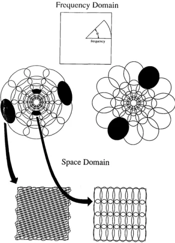
For the sake of clarity we will use the following

terminol-ogy to describe the Gabor coefficients.4 Each individual

function will be referred to as a sensor. A spatial array of

sensors tuned to the same spatial frequency will be referred to as a channel. For example, in Fig. 1(d) each of the

indi-vidual rectangles is a sensor. A row of rectangles is a chan-nel.

Therefore a narrow-band channel consists of a small num-ber of spatially large sensors, and a broadband channel con-sists of a large number of spatially restricted sensors. In the next section we consider the more general case of two-di-mensional frequency and space-limited functions; a channel

(a) ₍ _{Fourier transform}

Image

THE MODEL

This model shares a number of features with several recently developed models.4""1 2 The important feature of this par-ticular model is that it provides the freedom to vary the parameters of the components (e.g., the spatial-frequency bandwidth or the orientation bandwidth of the theoretical

cells) without losing information or adding free parameters.

The foundation of the model is derived from principles discussed by Gabor14and the principles of information

the-ory.2 6 Some of the basic ideas are represented in the infor-mation diagram shown in Fig. 1.

Consider a simple one-dimensional pattern consisting of 18 equally spaced pixels. In such an image, all the

informa-tion is represented by the amplitudes of the 18 pixels. The

information represented by such a pixel code can be repre-sented by the information diagram shown in Fig. 1(a). A pixel is a function that is localized in space but extends in

frequency (i.e., broadband). This property is represented

by each rectangle in the diagram.

It is also possible to represent the information in this

simple image by means of a discrete Fourier transform. Again, all the information is represented by 18 independent

coefficients (i.e., the amplitudes of 9 sine functions and 9 cosine functions). Each of these functions is localized in frequency but extends in space [Fig. 1(b)].

Gabor's theory implies that one can also represent the information in terms of the amplitudes of functions that are

localized in both space and frequency. In Figures 1(c) and 1(d) such coefficients are represented by rectangles, where the area of each rectangle is constant. Hence, if the function is large in space, then it is small in frequency and vice versa. Such functions need not all be the same size in space or frequency. Figure 1(d) shows a common representation in

U V.L Sb E a1 a' Space Space Gabor codes (d) (c) U> a, La. Space E U a_a' V. I I Space Fig. 1. Information diagrams, as proposed by Gabor.14 These

diagrams represent the information carried by a one-dimensional array of elements. For example, (a) represents the information

carried by 18 pixels. Each pixel is localized in space but extends in

frequency. The Fourier transform (b) represents the same amount

of information with 18 sines and cosines. Each element is localized in frequoncy but extends in apace. (c) and (d) show Gabor codej in which the information is represented by elements that are localized

in both space and frequency. The area represented by any element

(3)

will then be defined as an array of sensors tuned to the same spatial frequency and orientation.

Finally, we use the term code to refer to the entire collec-tion of channels (and therefore sensors) required to repre-sent the image. All the codes to be compared in this paper have roughly the same total number of sensors. This total

will equal the number of pixels in the original image.

Two-Dimensional Patterns

For a two-dimensional image, the trade-off in space and frequency is a bit more complicated than in the

one-dimen-sional case. Such two-dimenone-dimen-sional codes have been dis-cussed elsewhere.4"12 However, a few points should be made

about two-dimensional sampling and the trade-off between space and spatial frequency. A two-dimensional, vertically oriented Gabor function (i.e., a sensor) is defined by the

following equation:

g(x, y) = expl-[x2/2(AW)2 + y2/2(AL)2]jcos(2irfx + 0), (1) where AL denotes the spatial size of the sensor along its length (i.e., the axis parallel to the preferred orientation) and A W represents the width of the sensor in space (orthog-onal to the preferred orientation). As noted, the sampling distance in space (i.e., spacing between sensors) and the frequency (i.e., between channels) is proportional to the size of the function in space and frequency. In the two-dimen-sional case, the length of the sensor determines the spacing in the length direction. Furthermore, the orientation band-width of the function is inversely proportional to length, which in turn determines the spacing in the frequency do-main. In other words, the orientation bandwidth deter-mines the following parameters of the code: the distance (in the frequency domain) between neighboring orientation

channels, the number of orientation channels, the length of the sensor, and the separation between neighboring sensors in the length direction. Thus, if the code consists of chan-nels that are narrowly tuned to orientation, then it must sample at a relatively larger number of orientations.

How-ever, since the sensors of such a channel are relatively long, the sampling in space will be coarse.

In a similar manner, the width of the sensor (AW) mines the spacing along the width. The width also deter-mines the spatial-frequency bandwidth and hence the num-ber of channels required at different spatial frequencies. These points are also developed in greater detail in Figs. 2

and 3.

Relative Bandwidths

Another feature of this model is that, on a linear scale, the bandwidths of the different sensors are proportional to their

optimal frequencies. The overall design may be best de-scribed in terms of a rosettelike pattern as shown in Fig. 3.

This pattern shows how the two-dimensional frequency plane is divided. The center of this rosette represents a

frequency of zero (f = 0). Moving out from the center

represents an increase in frequency. The preferred

orienta-tion of the channel is represented by the angle from horizon-tal. As in Fig. 2, a single channel is represented by a pair of ellipses that are diagonally opposed. In both of the codes

represented in Fig. 3, the orientation bandwidth and the spatial-frequency bandwidth of the channel increase as a

function of the frequency to which the channel is tuned. This produces a code in which the orientation bandwidth is

constant in degrees and the spatial-frequency bandwidth is

constant in octaves.

Frequency Domain Space Domain

Fig. 2. Relations between the size of the channel in the frequency domain and the size and spacing in the space domain. A channel

with a bandwidth AF (frequency domain) consists of an array of sensors with a width AW (space domain). The spacing along the

width ASW will be proportional to the width AW. A channel with an orientation bandwidth AO (frequency domain) consists of any

array of sensors with a length AL (space domain). The spacing

along this length (ASL) will be proportional to the length.

Frequency Domain

frequcqcy

Space Domain

Fig. 3. Relations between the spacing of the channels in the

fre-quency domain and the spacing of the sensors in the space domain.

The upper two rosettes represent two possible coding schemes.

Both codes consist of channels that have constant spatial-frequency bandwidths in octaves and constant orientation tuning in degrees. The rosette on the left consists of channels that are more broadly tuned to orientation and more narrowly tuned to frequency than those of the rosette on the right. The bottom two diagrams give a

rough idea of the relative spacing of the sensors for two of the channels.

F

"----'.

(4)

The diagrams at the bottom of Fig. 3 give a rough idea of

the spacing of the individual sensors within each channel.

Sensors tuned to low frequencies are large in space, and therefore sampling in space is relatively coarse. Sensors

tuned to high frequencies are relatively small in space, and

therefore sampling is relatively fine. Each ellipse in space represents the relative size of a particular sensor. Again, the

bandwidth of the channel is inversely related to the size of

the sensors associated with the channel:

AF = k1/AW = k2/ASW, (2)

AO = k,/AL = k2/ASL. (3)

The number of sensors associated with a particular channel (NI/) is therefore proportional to the size of the channel:

N,1, = 1/(ASWASL) = (AFAO)/k. (4) Also, since the number of channels N, required to cover the two-dimensional frequency domain is inversely proportional to the bandwidths of the channels (i.e., AFAO), the total

number of sensors N0t will be constant:

N =t = NAI, = ca(AFAO)/(AFAO) = constant. (5) The precise details of the sampling scheme are not dis-cussed here, since they are not critical to the conclusions of

this paper. However, it must be reemphasized that the total

number of sensors is constant and is equal to the number of

free parameters in the input (i.e., the number of pixels).

(b)

Phase

Finally, we must consider the relative phase of the sensors.

In this version of the model, we will assume that at each

sensor location there exist two orthogonal phase-selective sensors (i.e., in quadrature). Pollen and Ronner2 7 have

shown that adjacent simple cells demonstrate such a

proper-ty. As has been noted,8"12their results do not suggest that the receptive field profiles must necessarily be even and odd

symmetric [0 = 0, 7r/2, -r, 37r/2 in Eq. (1)]. Indeed, the evidence supports a wide range of symmetries. 8 However, as long as the two phase relations are in quadrature (i.e., they differ by 90 deg), it is not critical what phases are involved.

The information provided by such a pair of cells is best described in terms of a two-dimensional vector whose length

provides information about the contrast energy at any given point and whose direction determines the phase of that

energy. For example, consider the response of a particular pair of such sensors to a sine-wave grating. The relative outputs of the two orthogonal sensors will depend on the positions of the pair of sensors relative to the grating. If we consider the vector sum of the outputs of the two sensors,

then the direction of the vector will oscillate as we move

across the grating, indicating a change in phase, but the length of the vector will remain roughly constant. The mag-nitude of this constant response will depend on the relation-ship between the spatial frequency of the grating and the frequency response of the channel.

This description will prove important for our consider-ations of response variability discussed in later sections.

I' ri _{M I}_'*JT_' A

4 IN

*4k, . 2i ' q .1% b i (a) (c) (d)

Fig. 4. The envelope of the response of one channel. Some of the calculations in this paper are based on the envelope of the response of the sensors. This envelope is sometimes referred to as the amplitude of the analytic signal28or the energy-density waveform.2 9 (b) The response of an even symmetric channel to the image in (a). (c) The response of an odd symmetric channel tuned to the same frequencies and

orientations. (d) The envelope, representing the root mean square [Eq. (6)] of the images in (b) and (c). The envelope takes into account both

the real energy and the reactive energy of the image28and thus permits a measure of the energy at a given location within a particular

orientation and frequency band, independent of the phase of the individual sensors.

(5)

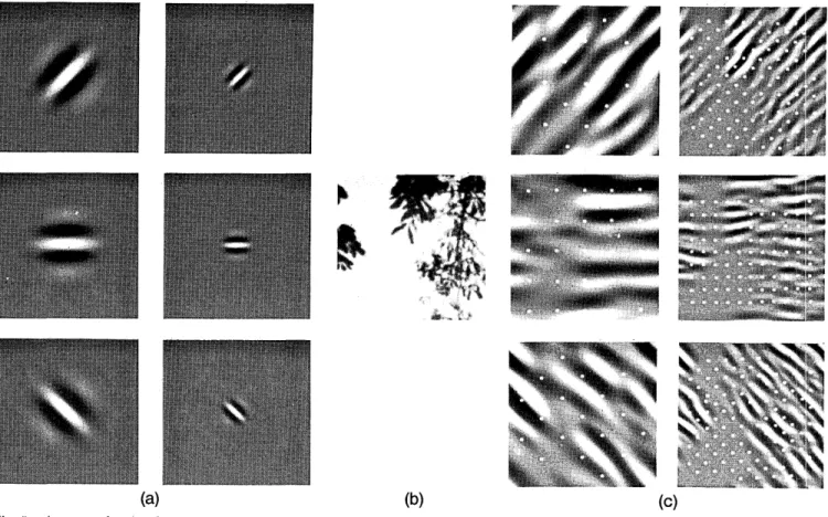
(a) (b) (c)

Fig. 5. An example of coding with six different channels. _{(a) Examples of the six types of sensor associated with each channel.} _(c) Convolution of the image in (b) with the six sensors shown in (a). The response of the individual sensors is determined by sampling these fil-tered images at a distance proportional to the size of the sensor (shown with dots). This diagram shows the response of only the even symmetric sensors. A complete code would involve the odd symmetric responses as well as the full distribution of orientations and spatial frequencies.

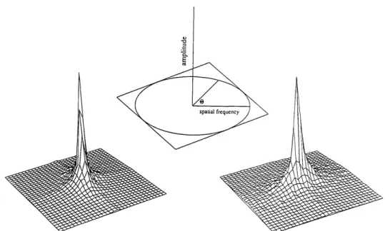
Our method of measuring the vector amplitude is shown in

Fig. 4. Figure 4 shows an example of a particular image [Fig.

4(a)] and the image when filtered through an orientation-and frequency-selective channel with even [Fig. 4(b)] orientation-and

odd [Fig. 4(c)] symmetry. Figure 4(d) shows the envelope

E(x, y) of these two orthogonal images, where

E(x, y) = [R(x, y)2+ I(x, y)2]1/2. (6) Such an image shows how the length of the vector (the

energy envelope) varies as a function of the position of the

pair of sensors. Just as the amplitude spectrum shows the response as a function of frequency that is independent of the phase, the envelope E shows the response as a function of position that is independent of the phase. Such a function is not unique to this study. It is generally described as the amplitude of the analytic signal2 8_{or as the square root of the} energy-density waveform.2 9 (The function also shows inter-esting similarities to the behavior of cortical complex cells.) In Section 3 we shall compare the variability of the re-sponses of different types of channels to a particular image. However, the periodicity introduced by bandpass filtering an image can create a spurious contribution to this

variabili-ty. Consider the filtered images in Figs. 4(b) and 4(c)

result-ing from filterresult-ing with the even and the odd symmetric channels. The periodicity in the filtered image is due to a

rotation of the response vector (i.e., a change in the local

phase) rather than to a change in the magnitude of the vector. The envelope provides a measure of the channel's response that is independent of this local phase change.

Overview

The main points of the model are described below and

illus-trated in Fig. 5:

(1) In the frequency domain, the distance between neighboring frequency channels is determined by the spa-tial-frequency bandwidth, which also determines the width of the individual sensors and hence the spacing along the width of the sensors

(2) In the frequency domain, the distance between neighboring orientation channels is determined by the ori-entation bandwidth, which also determines the length of the individual sensors and hence the spacing along the length of the sensors.

(3) Spatial-frequency bandwidths are constant in oc-taves, and orientation bandwidths are constant in degrees, but there is freedom to choose the absolute magnitudes of these bandwidths.

(4) At each position there are two orthogonal sensors with phase relations in quadrature. A response envelope

can be determined from each pair of sensors.

(5) The total number of sensors is independent of the particular choice of spatial-frequency or orientation

band-width (i.e., an image consisting of 65,536 pixels is represent-ed by 65,536 sensors).

In the following sections we look at the advantages of using such codes to represent the various types of images.

Ia

2

li,111

David J. Field

(6)

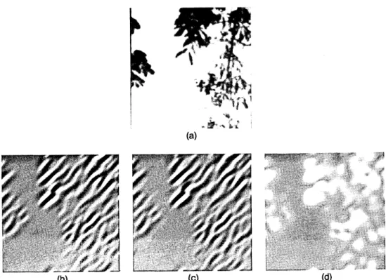
IMAGE ANALYSIS Methods

The six scenes used in this study were photographed with a Keystone 3572 camera (35 mm) using XP1 Kodak mono-chrome film. The scenes were taken from various places around England and Greece. No attempt was made to se-lect particular types of scene, but images were chosen that

had no artificial objects (buildings, roads, etc.). Although it

was hoped that these scenes were typical natural scenes, no effort was made to ensure this, and they may therefore rep-resent biased samples.

The negatives were digitized on a laser densitometer (Joyce Loebel) into 256 X 256 pixels with a depth of 8 bits/ pixel (256 density levels). The images were analyzed on a

Sun Workstation computer using conventional software de-veloped by the author.

Calibration

The modulation transfer function (MTF) of the optical

sys-tem (lens and developing process) was determined from the response of the system to a point source. A photograph of a

point source was taken with the same camera and film, and

the negative was developed in the same manner as the six

natural scenes. The results described below were corrected in accordance with this MTF.

IMAGE ANALYSIS: AMPLITUDE SPECTRA OF NATURAL IMAGES

In this section we discuss a particular property of natural

images as illustrated by their amplitude or power spectra.

This topic is discussed in greater detail in another paper. However, since the conclusions of this section play an impor-tant part in the next section, it is discussed briefly here.

Natural images, on the whole, appear to be rather com-plex. They are filled with objects and shadows and various

surfaces containing various patterns at a wide range of

orien-tations. Amid this complexity, it may seem surprising that such images share any consistent statistical features.

Con-sider the six images shown in Fig. 6. Such images may seem widely different, but as a group they can be easily distin-guished from a variety of other classes of image. For

exam-ple, random-dot patterns are statistically different from all

six of these natural images. This difference is best

de-scribed in terms of the amplitude spectra or power spectra of the images, where the amplitude spectrum is defined as the square root of the power spectrum.

The two-dimensional amplitude spectra for two of the six

images are shown in Fig. 7. The spectra of these images are

quite characteristic and are quite different from that of

white noise, which is by definition flat. They show greatest

amplitude at low frequencies (i.e., at the center of the plot) and decreasing amplitude as the frequency increases. The

f

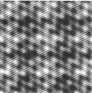
A B C

D E F

Fig. 6. Examples of the six images (A-F) in this study. Each image consists of 256 X 256 pixels with 256 gray levels (8 bits). However, only the central region was directly analyzed (160 X 160). See the text or details.

David J. Field

(7)

E

Fig. 7. Two-dimensional amplitude spectra for two images from Fig. 6 (A and D). The center of such a plot represents 0 spatial frequency.

Frequency increases as a function of the distance from the center, and orientation is represented by the angle from the horizontal. For the sake

of the clarity, each 256 X 256 amplitude spectrum has been reduced to 32 X 32. Thus each point in this plot represents an average of an 8 X 8

re-gion of the spectrum. Such plots show that amplitude decreases sharply with increasing frequency at all orientations.

amplitude falls off quickly by a factor of roughly 1/f (i.e., the

power falls at 1/f2). Figure 8 shows the amplitude spectra averaged across all orientations and plotted on log-log

coor-dinates.

Although the description is by no means perfect, these amplitude spectra are all roughly described by a slope of -1. This is not to say that all scenes from the natural world

would be expected to show a 1/f falloff; there are certainly scenes that do not show this property (i.e., a field of grass, the night sky, etc.). However, there are several reasons why

this 1/f falloff in amplitude should be expected to be a rough

average.

A 1/f falloff in the amplitude spectrum is what we would expect if the relative contrast energy of the image were scale invariant (i.e., independent of viewing distance). For

exam-ple, consider an image of a surface with an amount of energy

E between frequency f and frequency nf when viewed at a distance d. Increasing the distance by a factor a will shift the energy to the frequency range of af and anf. If we let the energy at any frequency equal

E(f) = g(f) * (2xf),

0.0

0.0 1.0 2.0

Loglo spatial frequency (cycles/picture)

Fig. 8. Amplitude spectra for the six images A-F, averaged across

all orientations. The spectra have been shifted up for clarity. On

these log-log coordinates the spectra fall off by a factor of roughly 1/f (a slope of -1). Therefore the power spectra fall off as 1/f2.

4.() 3.() U ei7 03 (7) 2.0 1.0 then to keep the energy constant in the range of all f to n/ for

all f requires

nf.

J

g(f) * (27rf)df = K,

Jfo

and it follows that

g(f) = k/f2.

(8)

(9)

In other words, if the power falls off as 1//2, there will be

equal energy in equal octaves. For example, the total energy

between 2 and 4 cycles/deg will equal the energy between 4

and 8 cycles/deg. (On a two-dimensional plot the area cov-ered by an octave band is proportional to f 2.) This falloff in power can also be related to the fractal nature of the

(8)

2386 J. Opt. Soc. Am. A/Vol. 4, No. 12/December 1987 4.() ;.() 0-c oI) l 2.( 0-1.0 -0.0 0.0 1.0 2.0

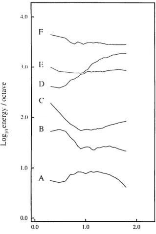
Logl0spatial frequency (cycles/picture) Fig. 9. Plot of energy per octave for each of the six images, for which energy is defined as the integral of the power spectrum

be-tween f and 2f. For example, the data at 10 cycles/picture

repre-sents the total energy between 10 and 20 cycles/picture across all

orientations. Although the results vary from image to image, these data suggest that, in contrast to the amplitude spectra, there is

roughly equal energy in any given octave. By Parseval's formula [Eq. (10)] this implies that the variance of the filtered image (fil-tered through a given octave) will be roughly constant. See the text for details.

nance profiles of the images, where the 1/f 2 falloff gives a fractal dimension of 2.5 (see Ref. 30).

Figure 9 shows the total energy in each 1-octave-wide

band as a function of the spatial frquency of the low end of the octave. These data suggest that, despite the variability from image to image, no particular band contains

consistent-ly more energy.

In terms of our model, this falloff in power proves quite important. Since, the channels have constant bandwidths

in octaves, as shown in Fig. 5, an image with a 1/#2 falloff in power will give roughly equal energy in each of the different

channels. Furthermore, by Parseval's theorem2 8the

vari-ance of the image is equal to the integral of the power

spec-trum, or, in the discrete case,

n-1

EIg'x)I2

n-1

X=0 =Z IG(f)12, (10)

f=0

where IG(f)12 represents the power spectrum.

Since the different frequency-selective channels in a given

code have constant bandwidths (in octaves), the outputs of the different channels will have roughly the same variance. If the statistics of natural images are also stationary (i.e., the statistics at any location in the visual field are no different from those at any other location), then all the different sensors will statistically have the same probability distribu-tion and therefore carry equivalent amounts of informadistribu-tion. Hence, with a 1/f2 power spectrum and an array of chan-nels with constant octave bandwidths and constant orienta-tion tuning (in degrees), the informaorienta-tion provided by each type of sensor will be roughly equal. Therefore the

rosette-like codes described in Fig. 3 permit the information in the image to be distributed evenly across the array of sensors.

To obtain some intuition of why this is so, consider that the profiles of sensors with the same bandwidth in octaves

are simply scaled versions of one another (i.e., they have the

same number of ripples, etc.). Images with 1/f amplitude spectra are also invariant in terms of their power at different

scales; that is, the amount of energy in any particular octave band is independent of the scale on which the image is

viewed. Hence coding a scale-invariant image into an array of scale-invariant sensors produces an even distribution of the information.

An even distribution may not seem to be an efficient

means of representing information in an image. Indeed, a

Karhounen-Loeve transform,2 5 which is often described as

an optimally efficient code, will result in an uneven

distribu-tion for images such as these. This is a point that we shall discuss below.

However, it is clear that having an even distribution is not

by itself a sufficient condition for an efficient code. Indeed, the information is evenly distributed with a pixel code if the image statistics are stationary. A code using channels with constant bandwidths in octaves will permit the different sensors to provide roughly equal information. However, the

efficiency of the code will depend on other parameters of

these channels. A constant bandwidth does not restrict us to any particular bandwidth (e.g., 1 versus 2 octaves). For

example, both of the codes shown in Fig. 3 have constant

octave bandwidths. In the next section we consider how the values of these bandwidths affect the efficiency of the representation.

IMAGE ANALYSIS: ENERGY DISTRIBUTION

In this section we compare various coding schemes in terms of the way that they represent the six natural images shown

in Fig. 6. The codes that will be compared will all fall within

the general constraints of the model described earlier. However, within these constraints, it is possible to compare the advantages and disadvantages of codes that involve vari-ous bandwidths.

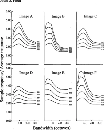
The main parameter that we will consider in this section is the variability of the responses of the arrays of sensors in the various channels. It was noted in the previous section that the variance in the outputs of the different channels will be roughly constant, independent of the channel that is select-ed. What, then, are the possible advantages of coding with a particular bandwidth? First, let us consider the rather

un-natural images shown in Fig. 10. As was noted previously, 2'

these two images are coded most efficiently with two quite

different codes. Image 1 consists of a number of points

E

F __

I) C B A David J. Field

(9)

Vol. 4, No. 12/December 1987/J. Opt. Soc. Am. A 2387 Image I 100r C. C> 0 C.) a Ce 0.75k l: i ,0.05 0.02 0.01 0.50k 0.25k 0.00 Image 2 I 1.0 2.0 1.0 2.0 Bandwidth (octaves)

scattered sparsely across the field. The probability of a point's existing at any given location is 0.01. What would be

an efficient code for a class of images such as this?

Consider a code in which only the nonzero coefficients are transmitted. If we code the image in terms of pixel values, then for this type of image only 1% of the coefficients are

needed to represent the image completely. Of course, infor-mation must be provided about the location of each

particu-lar nonzero coefficient, but as long as there are relatively few,

there are a number of ways of efficiently representing the sparse set (e.g., run-length coding25).

Now, suppose that we perform a Fourier transform of this dot pattern. The spectrum of such a pattern will be quite broad. Almost all the coefficients will be nonzero. There-fore, to code such an image, it would be necessary to transmit the amplitude of most of the Fourier coefficients. In this

sense, the pixel code can be described as an efficient code for

such images, whereas the Fourier transform would be an

inefficient code.

The opposite is the case for Image 2 of Fig. 10. This image consists of a small subset of sine-wave gratings of random

orientation and frequency. To represent this image by

us-ing pixels would require a high proportion of the available pixels. However, a Fourier transform of such an image will

Fig. 10. Energy distribution for two artificial images. Image 1 consists of random points with a probability of 0.01. Image 2

con-sists of 10 sinusoids. The plots shown at the bottom of the figure

describe the energy (as measured from the variance in the

respons-es) represented by different subsets of sensors in relation to the total

energy. Consider the data from Image 1 when the bandwidth is 1

octave. To get the data for this plot, the image was filtered through

a rosette of 1-octave-wide channels (circular in the frequency do-main: AF/AO = 1.0). The responses of the individual sensors and

the envelope were then determined by appropriate sampling. The

lowest curve labeled (0.01) shows the relative energy of the top 1% of the most active sensors. For Image 1, 1% of the sensors code about 20% of the total variance when the bandwidths of the channels are 1 octave, while 2% of the sensors code about 35% of the variance. The data for Image 1 show that more of the total variance can be

repre-sented with a small subset of the total sensors when the bandwidths

are broadest. In contrast, for Image 2 more variance can be

repre-sented by a small subset of the total sensors when the bandwidths are narrowest.

result in only 10 nonzero coefficients of a possible 65,536. Clearly, for the class of images consisting of randomly

select-ed sine-wave gratings, the Fourier transform is the most

efficient code.

But what of our natural images? Within the constraints

of our model, how can we design our code so that most of the

information is packed into the smallest number of active sensors? The analyses described below were designed to test this.

Methods

All analyses described in this section were performed on the

six 256 X 256 images described earlier and the two unnatural images described above. In all cases, the image was coded

by arrays of sensors tuned to a range of frequencies and orientations within the constraints of the model described earlier. The procedure involved computing a discrete Fou-rier transform (DFT) of the image, multiplying the DFT by the appropriate channel, performing an inverse DFT, and sampling this convolved image in proportion to the sensor size (inversely proportional to the channel size). Both the even and the odd symmetric responses are determined,

pro-viding a measure of the evelope [Eq. (6)]. Because the edges of the image can produce spurious output in a filtered image, David J. Field

(10)

only the central 160 X 160 pixels were directly analyzed; that

is, the center of any particular sensor did not exceed this

central region. However, depending on the size of this

re-gion, the sensors may extend out of it.

Even with this constraint, though, it was necessary to limit the analysis to channels centered above a particular

frequen-cy. This is because we wish to compare the behavior of

codes with different bandwidths, including rather narrow bandwidths. A sensor tuned to low frequencies with a rela-tively narrow bandwidth has a large size relative to the image. Even with the border described above, the edges can

have a significant effect. Because of this, the range of

fre-quencies to which the channels were tuned was limited to the range of 24-128 cycles/picture width (128 is the Nyquist

frequency for the 256 X 256 images). Thus, from the 25,600 possible sensors (160 X 160), roughly 20,800 sensors were

used in the analysis described below.

The spatial-frequency bandwidths of the channels will be defined in relation to the width at half-height. In particu-lar, the spatial-frequency bandwidth is defined as

Boct = log2(fa/fb), (11) where fa and fb represent the frequencies at half-height above and below the peak spatial frequency.

With the exception of that for Fig. 13 below, the width/ length aspect ratio of the channels (AF/AO) will remain fixed at 1.0. Thus the channels will be circular in the two-dimen-sional frequency domain.

The results described below are derived from the variabili-ty (i.e., the variance) of responses of the different sensors in a given code. To estimate this variability, it is important to

have a sufficiently large sample of the different sensors.

Beyond this, the precise nature of the sampling is unimpor-tant to estimating the total variance. The estimate is not dependent on the precise degree of overlap between neigh-boring channels or neighneigh-boring sensors. It is important only that the number of sensors within a particular channel be inversely proportional to the channel size.

Results

To help to understand the analyses described in this section,

let us first consider the images in Fig. 10. It is possible to

represent such images by using the computational model described above. The amplitude spectra of such images do not fall off as 1/f, and so different channels do not provide equal information. However, the general point can still be made.

The response of a particular channel can be defined in terms of the variance of the filtered image. As noted earlier, for the rosettelike codes the variance of the different

chan-nels will be roughly constant. However, a given variance can

be produced by a range of different response distributions.

For example, when a pixel code is used with Image 1, most of

the response variance of the channels comes from the large responses of relatively few sensors. With the Fourier code,

the overall variance (i.e., the power) comes from the general-ly low activity of a large number of coefficients.

The pixel code is efficient because most of the variance in the population of sensors is due to the response of relatively

few sensors. Figure 10 provides a measure of the proportion

of the variance represented by the most active sensors, as a function of the bandwidth (in octaves) of the code. For

example, a particular code is chosen (within the constraints of the model) with a particular spatial frequency and

orien-tation bandwidth (e.g., 1 octave, 20 deg). The code is then applied to the image, which results in a distribution of

re-sponses in the sensors. We can then consider the rere-sponses of the most active, say, 20% of the sensors and determine how much of the variance is accounted for by this subset. The

plots in Fig. 10 show how much of the total energy is account-ed for by the top 20, 10, 5, and 1% of the sensors.

Figure 10 shows that for Image 1, as the bandwidth of the code increases, the most active sensors account for higher and higher percentages of the total energy. In contrast, for Image 2, the most energy is packed into the fewest number of cells when the bandwidths of the channels are narrowest.

With this definition, the efficiency of the code is a

func-tion of both the parameters of the code and the statistics of the image. But what is the optimal solution for natural

images? Figure 11 shows the results for our six images. The results for each of the six images in Fig. 11, with the

possible exception of Image E, show the same general trends. The optimal bandwidths are neither very narrow or very broad but are in the range of 0.5 to 1.5 octaves. In other words, in order to represent the maximum energy with the fewest sensors, the optimal solution within the constraints of the model is to use sensors in the range of 0.5 to 1.5 octaves. If the energy of the image is represented primarily by a few of the total sensors, we would expect the response of these few sensors to be high relative to the average. Figure 12 shows the average response of different subsets relative to the average response of the population. These data show that when the bandwidths are about 1 octave, the most

°00r 0.75 0 E5 ._ d) a Ce M 1X Ce 0 CZ Ce 0.50 0.25 0.00 1.00 Image A 0.20 0.10 0.05 0.02 0.01 Image D 0.75k 0.50 /--_0 .20 0 .10 0.25 0.05 0.02 0 . 0 1~~~~~~00 .0 o 3.00 1.0 2.0 3.0 Image E 0.20 \ __ _ 0.10 0.05 0.02 0.01 1.0 2.0 3.0 Image C 0.20 0 .10 11" 00.05 f - g g ,~~~~~0.2 Bandwidth (octaves)

Fig. 11. Energy distribution for the six natural images. Results

show the energy represented by different subsets of sensors. Re-sults are shown for the range of 0.12-3.2 octaves. The ratio of

orientation bandwidth to spatial-frequency bandwidth (AF/AO) is

fixed at 1.0 (i.e., circular channels).

(11)

Vol. 4, No. 12/December 1987/J. Opt. Soc. Am. A 2389 6.00-Image A X~~~~~~~~~~. Ia II Image D I aatM II. II. 1.001 0.0 , I.1.0 2.0 3.0 Image B Image E 1.0 2.0 3.0 1.0 2.0 3.0 Image C G i~~~~~~~~~~~~~~~(." 11., ,) 0

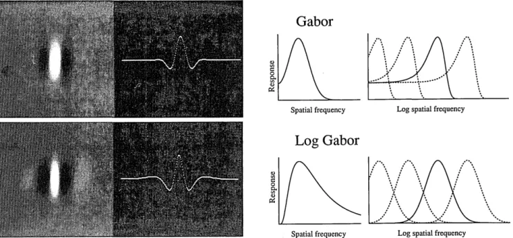
natural images. Gabor codes have a number of interesting mathematical properties. As described by Gabor14 and more recently by Daugman,12a Gabor function represents a minimum in terms of the spread of uncertainty in space and spatial frequency (actually time and frequency in Gabor's description). However, the Gabor code is mathematically pure in only the Cartesian coordinates where all the Gabor channels are the same size in frequency and hence have sensors that are all the same size in space (i.e., all the rectan-gles in the diagrams in Fig. 1 are the same size). In such a case, the Gabor code represents the most effective means of packing the information space with a minimum of spread and hence a minimum of overlap between neighboring units in both space and frequency.

However, modifying the basic structure of the code to permit a polar distribution such as that shown in our rosettes (Fig. 3) alters the relative spread and overlap between neigh-bors. In this section some results are described that were obtained with a function that partially restores some of the destructive effects of the polar mapping. This function will be called the log Gabor function. It has a frequency re-sponse described by

G(f) = expi-[log(f/f0)]2/2[log(oi/f0)]2I, (12)

Bandwidth (octaves)

Fig. 12. Relative response of the different subsets of sensors as a

function of the bandwidth. For example, the plot labeled 0.01 represents the average response of the top 1% of the sensors relative to the average response of all the sensors. If we consider the sensor response to be subject to noise, then this plot can be related to the signal-to-noise ratio. It suggests that spatial-frequency

band-widths in the range of 1 octave produce the highest signal-to-noise

ratio.

active sensors have a high response to the average. If we consider the fact that cortical neurones are inherently rather noisy in their response to a stimulus,3' this plot can be considered a measure of the signal-to-noise ratio of different types of sensors. Coding information into channels with approximately 1-octave bandwidths produces a

representa-tion in which a small proporrepresenta-tion of the cells represents a

large proportion of the information with a high signal-to-noise ratio.

We have so far considered only channels for which the

ratio of the spatial-frequency bandwidth to the orientation

bandwidth is constant (AF/AO = 1.0). Figure 13 shows

re-sults with various different aspect ratios. One of the diffi-culties of such an analysis is that the two-dimensional Gabor functions are not polar separable. That is, the spatial-fre-quency tuning is not independent of the orientation tuning (in degrees). Extending the orientation bandwidth actually extends the response of the channel to higher frequencies. With the 1/f amplitude spectrum, the response of the chan-nel will be dependent primarily on the lower frequencies, with little effect produced by the extension. Nonetheless,

the results of such an analysis are shown in Fig. 13. As can

be seen, an aspect ratio of about 0.5-1.0 is somewhat opti-mal, although the effects are small.

LOG GABOR CHANNELS

In the previous section we compared a variety of Gabor codes in terms of their ability to represent the information in

that is, the frequency response is a Gaussian on a log

fre-quency axis. Figure 14 provides a comparison between the

6.00r 0.) 0 0~ C,, VI) 2-02 to 2-0) 0 C, 0 0.) 2-0.) Ca. E_c V) Image A 5.00 -4.00 -0.0o 0.02 3.00 0.05 0.10 2.00 1.00 0.00 6.00 Image D 5.0 -4.00k 3.00c 2.00 __ _~ 0.02 0.0 - . ..--- - 0.10 0.20 1.0C 0.00' 0.25 1.00 4.00 Image B 0o,0 002 0.05 0.20 Image E 0.01 0.02 0.05 \ 0.10 0.20 0.25 1.00 4.00 Image C 0.02 0.05 0.10 _~~0.20 Image F 0.02 0.02 0.05 0.20 0.20 0.25 1.00 4.00

Spatial frequency bandwidth / Orientation bandwidth Fig. 13. Relative response of the different subsets as a function of the ratio of the orientation bandwidth to the spatial-frequency

bandwidth (AF/AO). A ratio of 1.0 represents a channel that is circular in frequency space. A ratio of 0.25 represents a channel

that is narrowly tuned to orientation realtive to the spatial-frequen-cy tuning. For all plots shown here, the spatial-frequenspatial-frequen-cy

band-width is fixed at 1.2 octaves.

David J. Field 5.00 4.00 d. 3.00 coo 0 I 2.00 r~2 0 1.01 to 02 > 0.0c ¢oX 6.OC ar 0 1=,a s.oc 2 4.OC 0) E. 3.OC 2.OC 11 1,

(12)

Gabor

a) 0 W. Spatial frequency :1, 4 X

Log spatial frequency

Log Gabor

Spatial frequency Log spatial frequency

Fig. 14. Comparison of the Gabor and the log Gabor functions. The far left-hand images show examples of the two functions in their even symmetric form along with the response amplitude across the midline. The amplitude spectrum of a Gabor function is represented by a sum of Gaussians (positive plus negative frequencies) and will be roughly symmetric on a linear axis. The log Gabor is a Gaussian on a log frequency

axis. The channels in our rosettes have constant bandwidths in octaves, and therefore the amplitude spectra of the different channels will the

the same scale on the log frequency axis. As shown by the plots on the right, the Gabor functions overrepresent the low frequencies with this type of sampling. This is not the case for the log Gabor.

Gabor function and this log Gabor function. The important aspect of this function is that, unlike the Gabor function, the

frequency response of the log Gabor is symmetric on a log

axis. Indeed, the log axis is the standard method for repre-senting the spatial-frequency response of visual neurones. The results of several studies seem to imply that such sym-metry is strong possibility. Recent work by Hawken and

Parker3 2 suggests that the Gabor function fails to capture the precise form of the spatial-frequency tuning curves in

monkey cortical cells. In their detailed study, a number of

models are compared for their ability to predict the form of

the spatial-frequency tuning curve. Gabor functions miss in this fit primarily because they fail to capture the relative

symmetry of the tuning curves on a log axis. This does not

mean that the log Gabor is the best-fitting function

(Haw-ken and Parker actually suggest a model based on a sum of weighted Gaussians), but it may well provide a better

de-scription than the Gabor function.

One of the advantages of the log Gabor is its use with codes in which the bandwidths increase with frequency (i.e., are constant in octaves). The right-hand side of Fig. 14 shows a

one-dimensional representation of the spacings of the Gabor

function on a log axis. With the bandwidths constant in

octaves, the Gabor functions overrepresent the low frequen-cies. Furthermore, with a 1/f falloff in the amplitude, most

of the input to the Gabors will be provided by the

low-frequency tails of the functions. This will, in essence, pro-duce a correlated and redundant response to the low fre-quencies. In contrast, mapping the information into the log Gabors spreads the information equally across the channels.

Figure 15 shows the results of the log Gabors (solid lines) compared with the Gabors (dashed lines) obtained by using

the methods described in the previous section (Figs. 11 and

12). For bandwidths of less than 1 octave, the two functions

produce similar results. At bandwidths of >1 octave, the redundancy at the low frequencies becomes apparent. Since all the Gabor sensors receive a significant and redun-dant input from the low frequencies, the responses of any given sensor represents a smaller fraction of the total energy. The frequency response of the log Gabor code permits a more compact representation than the Gabor code when the bandwidths are >1 octave. The log Gabor may not be the ideal function for coding images, and it is probably not the ideal function for representing cortical simple cells.

Howev-er, its success with broad bandwidths may help to explain why the frequency-response functions of many cortical cells

are symmetric on a log axis.

0) CZ C's 0 CZ C's 0) 0. E CZ V) Average A - F 0.75j 0.50 0.25 I d

~~~~~~~0.20

) 0 . 1~~~~~~~0. > 7 ' 0.05 / A -_

~~~~~~0.01

a) 0 In r_ 0 M. 01) 10) to Mu 0 d') 0 ¢ 0 0.0) ~2 0. Eo Co 0.00' _1.0L _2.02 _3.03 6.0r 5.01. 4.0-3.0 2.0 Average A - F 1) 21) I . . . 121) 1.0 F 0.0' I 1.0 2.0 3.0 Bandwidth (octaves)

Fig. 15. Comparisons of the Gabor and log Gabor functions for

coding the six natural images. Each plot shows the average result

for the GTabor functions from Figs. 11 and 12 (dashed lines) and for log Gabors (solid lines). With bandwidths greater than 1 octave, the log Gabor shows the potential of producing a more compact code. 0) 0 0. 0) David J. Field 1.00r

(13)

DISCUSSION

Over the past two decades, a number of attempts have been

made to explain the purpose of the rather mysterious behav-ior of cortical neurons. The evidence that cortical neurons

are selective to spatial frequency as well as orientation

di-rected a number of researchers to suggest that such neurons must be producing something like a Fourier transform and not performing feature detection.3 3'3 4 Features were as-sumed to be things such as edges, bars, and corners. The

frequency selectivity of cortical cells seemed to be in

opposi-tion to the noopposi-tion of feature detecopposi-tion because frequency selectivity seemed to have little to do with the properties of the natural environment.

We have tried to show in this paper that the response properties of cortical neurons are well suited to the statistics of natural images. The frequency selectivity allows the

im-ages to be represented by a few active cells. One might say

that sensors with the tuning of cortical cells provide the best

chance of giving a large response or no response at all. How-ever, one should be hesitant in describing such behavior as

feature detection. No mention has been made of what sta-tistics of the environment might be biologically significant to the animal. No effort has been made to give preference to

any particular object or event in the environment. We

sug-gest instead that the code allows, on the average, the most information to be represented with a small proportion of cells. However, information is defined in relation to the variability of the images, not any specific feature.

We can also relate this description of information in terms

of the redundancy of the images. Barlow2 0-2 3has provided a

-thorough discussion of the relations between redundancy and visual codes. Indeed, many of the results described here may be discussed best in terms of Barlow's theories of redundancy.

The redundancy in a set of images is usually defined in terms of the nth-order conditional probabilities of the

coeffi-cients (e.g., the amplitudes of the pixels; see Ref. 18 for an excellent discussion). Consider an array of pixels with a range of possible intensity levels. First-order statistics re-late to the probability of individual pixels' (e.g., pixel i)

taking on particular intensity levels (m) - p(mi).

There is redundancy in the first-order statistics when the distribution of intensities is not uniform. A nonuniform

distribution implies that there is some degree of

predictabil-ity or order in the intenspredictabil-ity values.

Second-order statistics refer to the conditional

probabili-ty of pairs of pixels. It is a measure of the probabiliprobabili-ty that a pixel will take on a particular value given the value of anoth-er pixel, p(mil nj). Most considanoth-erations of redundancy

in-clude only the second-order redundancy portrayed in the power spectrum and the autocorrelation function. Howev-er, higher-order redundancy (e.g., third order) may provide a significant contribution to the total redundancy of an image. Consider an image consisting of small line segments of

ran-dom orientation. In such an image, if we find two

neighbor-ing points with the same intensity, then it is likely that there will be a third point along the line with the same intensity. This correlation can be described as a third-order statistic, since it concerns the relation between triplets of points p(msi ni, o0). The power spectrum and the autocorrelation func-tion provide no informafunc-tion about this third-order statistic. How should we represent these various forms of

redun-dancy? Barlow suggests that the ultimate goal is to reduce the redundancy of the code. Does the model proposed here reduce redundancy? The answer is clearly no. The total number of sensors has remained fixed, and the amount of

information represented by the code is constant (for a

com-plete code). Thus the order in the code has been main-tained, and therefore the total entropy or redundancy is

constant.3 5

Instead, the code presented here provides a means of con-verting higher-order redundancy (correlations between pairs of pixels, triplets of pixels, etc.) into first-order redun-dancy (i.e., the response distribution of the sensors). Theo-retically the total redundancy will be unchanged.

For example, consider Image 2 of Fig. 10. If we code such an image in terms of pixels, then there will be a fairly even

distribution of responses. An even distribution implies that the entropy is relatively high and that the redundancy or

predictability is low; that is, no particular response is more or less likely than any other. The redundancy of such an

image lies in the correlations between neighboring pixels. A Fourier transform of this image transforms this second-or-der redundancy into redundancy in the response distribu-tion (first order). The Fourier coefficients are not evenly distributed. The most likely state is 0 with a small probabil-ity of a large response. Hence the first-order statistics are more predictable or redundant.

The response distributions represented in Figs. 11 and 12 can be interpreted in terms of the redundancy of the differ-ent codes. With a 1-octave bandwidth, the information is packed into the smallest number of sensors, giving a highly skewed distribution and therefore a redundant code. In other words, the most efficient code by our terminology is the code with most redundant first-order statistics.

The next stage of processing can make efficient use of

these first-order statistics by coding only the nonredundant elements (i.e., the highly active sensors). It is therefore the next stage of processing that has the potential for removing redundancy. The codes described here should be no more and no less redundant than the input.

Karhounen-Loeve Transforms

Bossomaier and Snyder36 recently discussed some of the similarities between the response properties of simple cells and the solution of a statistical analysis called a Karhounen-Loeve transform (KLT; e.g., see Ref. 25). Bossomaier and Snyder suggest that, in the same way that the KLT can be used to reduce redundancy, local spatial-frequency analysis may be the optimal procedure for removing statistical re-dundancy in real images. However, what they presume to be the goal of the visual code is not the same as that proposed here. The KLT computes the eigenvalues of the covariance matrix (i.e., the covariance between pairs of pixels). The corresponding eigenvectors represent a set of orthogonal coefficients for which the vector with the greatest eigenvalue accounts for the greatest part of the covariance.

The KLT is used to represent the information from a class

of images (or blocks within an image) as a hierarchy of orthogonal coefficients in which most of the image energy is

represented consistently by the same small subset of coeffi-cients. By using only this small subset, it is possible to code most of the energy in the images with a large reduction in the

number of free parameters. Redundancy is reduced by

(14)

ducing the dimensions (i.e., the number of sensors) of the code. As was noted by Snyder and Bossomaier,3 6 if the statistics of the images are stationary (i.e., across all the images, the statistics at any one location are no different from those at any other location), then the KLT produces coefficients similar to those of a Fourier transform. Indeed,

if we consider the amplitude spectra shown in Figs. 5 and 6,

it is clear that most of the energy can be conserved by

transmitting only the low frequencies. For images such as

these with power spectra that fall as a function of frequency, using the KLT to eliminate weak coefficients will remove the higher frequencies.

The code proposed in this paper behaves quite differently. The goal is not to discard any type of channel or sensor. The

coefficients are matched to the image energy (1/f2) so that, on the average, any particular coefficient (channel or sensor) is just as likely to be active as any other. No particular coefficient is favored by such a code. Hence there can be no

reduction in the number of free parameters. This code is efficient because the redundancy of the first-order statistics (i.e., the response distribution of the sensors) has increased. For any particular image, only a small subset of the total number is active. Since the particular members of the sub-set will vary from image to image, it is not possible to elimi-nate any particular type of coefficient. If the number of free parameters (i.e., the dimensionality) is constant, then the total redundancy should remain constant.

It is proposed here that this coding scheme (which is not a local Fourier transform) represents a good method for trans-forming higher-order redundancy into first-order redundan-cy. It is presumed that this redundancy is used in later stages to produce a nonredundant code. Indeed, if the later

stages analyze the outputs of only the very active cells (i.e.,

impose a threshold), then redundancy can be reduced.

However, this model of simple-cell behavior does not achieve

this. These results can only indirectly support Barlow's theory20-23 that the ultimate goal of visual processing is to represent visual information in a nonredundant form. By this model, cortical simple cells do not represent information with less redundancy. Instead they transform the informa-tion to permit later stages of the visual system to be less redundant.

We must limit ourselves to the claim that such a code is only a good method for transforming redundancy. We have only searched through two types of code (Gabor and log

Gabor). There might well be some other function that pro-vides a more efficient means of transforming redundancy and that might also provide a better description of the

neu-rophysiology.

Physiological Reality

A number of points must be addressed regarding the differ-ences between the idealized model proposed here and the coding by the mammalian visual system. Some differences (e.g., scaling factors from fovea to periphery) are not directly relevant to the model. However, there are at least four areas in which the known properties of the visual system appear to conflict with the model.

1. Precise Bandwidths and Spacing

Our results suggest that channels with a -1-octave band-width and an orientation/frequency bandband-width ratio of

around 0.8 will produce a relatively efficient representation of the information in these six natural images. This is in good agreement with the general neurophysiological

find-ings for spatial-frequency bandwidths in cortical simple cells

(e.g., Refs. 37 and 38) and with ratios averaging around

0.6.39,40 However, the various codes described here are based on an even distribution of channels and sensors (e.g., Fig. 3). The restrictions that were imposed permitted a comparison of different coding schemes. There is little rea-son to expect such precise coding in the visual cortex.

In-deed, a number of authors3 7'3 8 have pointed out the wide

distribution in the spatial-frequency and orientation band-widths of cortical neurons. Furthermore, it is unlikely that the spacing between cortical neurons is anything like the rigid grid proposed here. It remains unclear what effect

variability will have on the code. A wide distribution in the bandwidths may even produce a more efficient code by

pro-viding a wider selection of potential matches between the sensors and the image.

2. Noise

Actual cortical neurons are quite noisy, providing a rather inconsistent response to a constant stimulus. Although noise is not explicitly attached to this model, one might expect the model to work well with noisy cells (i.e., sensors).

As is shown in Figs. 11 and 12, when the bandwidths are in the region of 1 octave, the most active cells give the highest

response relative to the average. Thus, if there is noise associated with this average response, then this range of bandwidths will give the optimal signal-to-noise ratio.

3. Optics

The photographs that were analyzed in this study were each corrected for the optics of the camera. However, one might question whether the analyses should reflect the optics of the mammalian eye. Indeed, it was noted above that the constant bandwidth (in octaves) was well suited to the falloff

in energy of the images. A reduction in the amplitude of the

higher spatial frequencies will certainly effect the equal dis-tribution of information through the system. However, this should not necessarily imply that the optimal bandwidths

should vary as a function of frequency.41 As long as the

falloff is not too steep, then each channel's input will be modified only by an overall reduction in contrast. This reduction may decrease the signal-to-noise ratio for the high-frequency channels but should have little effect on which bandwidths produce the optimal ratio. However, it does imply that a threshold applied equally across the differ-ent channels is more likely to effect the channels reduced by the relative effects of the optical system.

4. Redundancy

So far, we have discussed redundancy as something to avoid

in a visual code. However, it is well known that redundancy

can be an advantage if the coding process is subject to noise. However, this is a second form of redundancy. The redun-dancy that we have discussed so far refers to the statistics and correlations of the input. In this sense, it is redundant

to code images of a point in terms of sinusoids because the

different slnusoids are redundant. A second type of redun-dancy refers to overrepresenting the information in a

stimu-lus by using more free parameters (i.e., coefficients) than are