Variations, and Applications
Claus Weihs, Swetlana Herbrandt, Nadja Bauer, Klaus Friedrichs, and Daniel Horn
Abstract A popular optimization method of a black box objective function is Efficient Global Optimization (EGO), also known as Sequential Model Based Optimization, SMBO, with kriging and expected improvement. EGO is a se-quential design of experiments aiming at gaining as much information as pos-sible from as few experiments as feapos-sible by a skillful choice of the factor settings in a sequential way. In this paper we will introduce the standard proce-dure and some of its variants. In particular, we will propose some new variants like regression as a modeling alternative to kriging and two simple methods for the handling of categorical variables, and we will discuss focus search for the optimization of the infill criterion. Finally, we will give relevant examples for the application of the method. Moreover, in our group, we implemented all the described methods in the publicly available R package mlrMBO.
1 Introduction
The overall goal of this paper is global optimization of factor settings by min-imizing an objective function. Exemplarily, such objective function may be a measure of a product or property of an algorithm, such as stability, yield,
Department of Statistics, TU Dortmund University, D-44221 Dortmund, Germany
[claus.weihs,swetlana.herbrandt,nadja.bauer]@tu-dortmund.de [klaus.friedrichs,daniel.horn]@tu-dortmund.de
AR C H I V E S O F DAT ASC I E N C E( ON L I N E FI R S T) DOI 10.5445/KSP/1000058749/01
K I T SC I E N T I F I C PU B L I S H I N G ISSN 2363-9881
or predictive power. Influencing factors may be ingredients, process settings, or algorithm’s parameters. Typical challenges are that the evaluation of the (black box) objective function is expensive (in money, storage, animal lives, etc.) and/or time consuming and that many different factor settings have to be studied to find the best settings. The solution studied in this paper is sequential design of experiments in order to gain as much information as possible from as few experiments as feasible by a skillful choice of the factor settings in a sequential way.
Let the design matrixX consist ofnsettings in the rows for pfactors (ingre-dients/parameters) in the columns:
X= x11· · · x1p .. . . .. ... xn1· · · xnp .
Let the objective function f(x)be a real-valued black box function with values f(xi) =yifor the ith settingxi= (xi1. . .xip)Tof the pfactors. Let the vector of
values of the objective bey= (y1. . .yn)T.
In classical design of experiments, an optimization design might be a bigger response surface design like a central-composite (Myers et al, 2009) or a space filling design (McKay et al, 1979; Cioppa and Lucas, 2007), or the like, directly evaluated by experiments or simulations. The results would be evaluated by means of a regression model, estimating the unknown parameters. Finally, opti-mum factor levels would be determined regarding the estimated model (Myers et al, 2009). Unfortunately, this procedure has at least two very important draw-backs: the time for carrying-out the, typically, many experiments and the need to repeat the whole procedure in case of a poor fit.
The iterative approach called Efficient Global Optimization (EGO) (Jones et al, 1998) also starts with an initial design which is evaluated directly by experiments or simulations. However, this design is typically a space filling design, which is much smaller than the classical response surface designs. Then, the experimental results are analyzed by means of an approximate (so-called surrogate) model, which can be evaluated much faster than an experiment or a simulation. A new design point is found by means of the optimization of a (so-called infill) criterion evaluating the estimated approximate model. This new design point is the next parameter setting directly evaluated by an experiment or a simulation. This step of model estimation and generation of a new design point is iterated until a stop criterion is fulfilled. The selection of surrogate models and infill criteria will be discussed in detail in this paper.
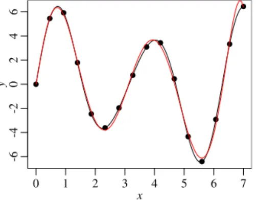
Example 1.Consider only one factorx(i.e.,p=1),x∈[0,7], and the true (in practice unknown) objective functiony= f(x) =sin(x) +2sin(2x) +sin(3x). The optimal factor value isx∗≈5.549. In the classical approach we typically as-sume a quadratic regression model. Here, we even asas-sume a higher order model, namely of 8th (!) order, to improve the approximation:y=β0+∑8k=1βkxk+ε.
As a design we use 16 equidistant points (see Fig. 1). Then, the best evaluated setting isx=5.6875 (minimum of the design points) and the best predicted set-ting ˆx∗≈5.586 (calculated minimum of estimated red curve in Fig. 1). There-fore, the predicted optimal argument is very close to the true optimal factor value x∗ ≈5.549 (see above, minimum of true black curve in Fig. 1). The question is: Can EGO produce even better results?
0 1 2 3 4 5 6 7 x -6 -4 -2 0 2 4 6 y
Fig. 1 Example function with 16 equidistant de-sign points (black dots), black line = true function, red line = estimated function. Note, how near the minima of the true and the estimated curves are.
The paper is structured as follows. In Sect. 2, the EGO procedure will be introduced. In Sect. 3, variations of this procedure will be discussed. Here, we will especially introduce our new variations of the EGO pro-cedure, namely regression as a mod-eling alternative to kriging, focus search for the optimization of the in-fill criterion, and two simple methods for the handling of categorical vari-ables. Sect. 4 presents applications to parameter tuning, onset detection, and cutting optimization. The paper finishes with a conclusion.
2 Efficient Global Optimization
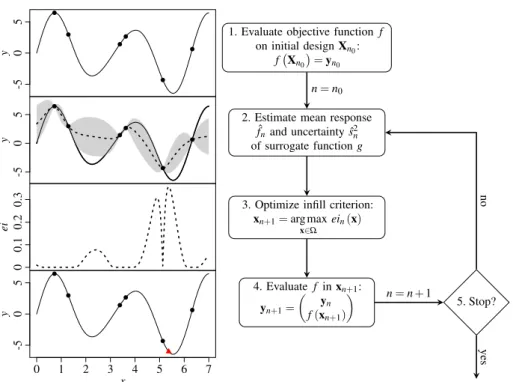
In this section, the EGO procedure will be described in detail. See Fig. 2 for an overview over the whole procedure. The steps of this procedure will be discussed in the following subsections.
y -5 0 5 y -5 0 5 ei 0 0.1 0.2 0.3 0 1 2 3 4 5 6 7 x y -5 0 5
1. Evaluate objective functionf on initial designXn0:
f Xn0
=yn0
2. Estimate mean response ˆ
fnand uncertainty ˆs2n
of surrogate functiong
3. Optimize infill criterion:
xn+1=arg max x∈Ω ein(x) 4. Evaluate f inxn+1: yn+1= yn f(xn+1) 5. Stop? n=n0 n=n+1 no yes
Fig. 2 Global optimization steps: On the left, an example is given (predetermined design points as black dots, new design point as a red triangle); on the right, the steps are briefly described (see the main text for a detailed explanation).
2.1 Initial Design
In step 1 of the EGO procedure, the initial design should be chosen small but nevertheless covering the whole region of interest from the outset. Also, if pos-sible, all factors should be considered which might improve the objective. From now on, we assume that the region of interestΩ=Ω1×. . .×Ωpof the factor
vectorx= (x1. . .xp)T is restricted by box constraintsΩj= [xj,lower,xj,upper]⊂
R.
In order to cover the whole region of interest to search for the best setting, typically, a space-filling design like a Latin hypercube design is used (McKay et al, 1979). ALatin Hypercube Design(LHD) is constructed so that each factor has the same number of levels. For each level of each factor there is exactly one design point. The idea is to divide the range of the pcharacteristics into n0 equally probable intervals, taking the center as the design level. Then,n0
0 1 2 3 4 5 6 7 x -6 -4 -2 0 2 4 6 y 1 2 3 4 1 2 3 4 1 2 3 4 x2 x1 x3 ● ● ● ●
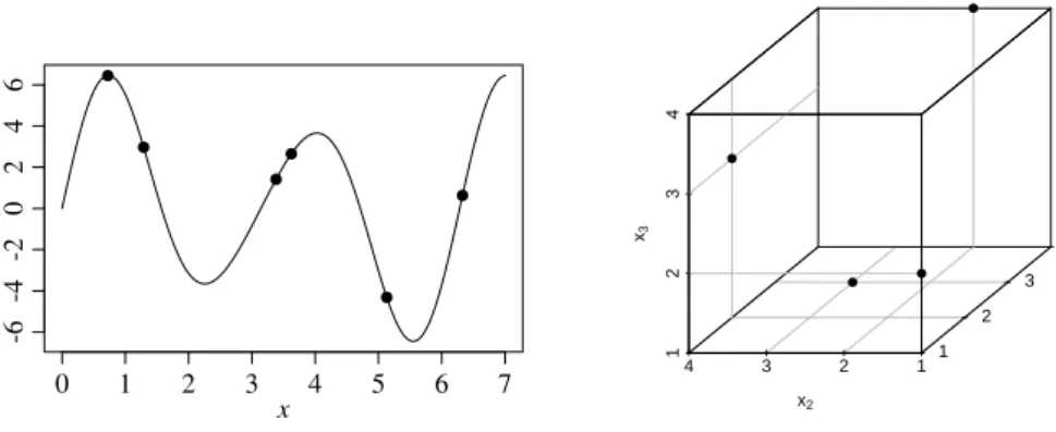
Fig. 3 Sine example function with 6 random design points (left); Latin hypercube design with 4 points (right).
design points are placed to satisfy the Latin hypercube requirements. Typically, the design is filled by a random permutation of levels factor by factor. Note that the number of divisions,n0, is assumed equal for each factor. Also note that this
design does not require more design points for more factors. This independence is one of the main advantages of this design. For the numbern0of initial design
points, typicallyn0∈ {5p,6p, . . . ,10p}is recommended.
Example 2 (Example 1 cont.). In the above example the region of interest is Ω = [0,7]. Let the initial design include n0=6p=6 points from a
ran-dom Latin hypercube with XT6 = (5.13 3.38 1.29 3.62 6.33 0.72) and
yT
6 = (−4.32 1.42 2.97 2.65 0.63 6.45)(see Fig. 3 (left)).
Example 3.An LHD for p=3 factors with n=4 design points in Ωj = {1,2,3,4}may look like this:
X4= xT 1 xT2 xT3 xT 4 = 1 1 2 2 4 3 4 2 4 3 3 1
(cp. Fig. 3 (right)). Obviously, each factor level appears once for each of the 3 factors.
2.2 Surrogate Function
In step 2 of the EGO procedure, a reasonable approximation g(x) of the un-known objective function is looked for. With this approximation we predict the objective for each factor setting. In order to determine this approximation, we consider an approximation model, also called surrogate model or meta model, g(x). For fast evaluation, we assume that this model is of simple form.
We first concentrate onordinary kriging(Cressie, 1988) with the surrogate modelg(x) =µ+Z(x). The constantµ can be interpreted as a global mean, andZ(x)is a Gaussian process withE(Z(x)) =0 and a stationary covariance Cov(Z(x),Z(x0)) =σ2ρ(x−x0,ψ) with, e.g., theMatérn 3/2kernel function ρ(x−x0,ψ) = (1+
√
3||x−ψx0||)exp(−√3||x−ψx0||)(Matérn, 1986). The constant
σ2 can be interpreted as the global variance,ψ as a scaling parameter, and
the Matérn kernel as a correlation function. A Gaussian process is a statistical model for observations in a continuous input space like time or space, where every point is associated with a normally distributed random variable and every finite collection of those random variables has a multivariate normal distribu-tion. As a measure of the similarity between points, their covariance is used, specified by a kernel function (we use the Matérn 3/2 kernel function). Predic-tion is not just a point estimate, but also includes uncertainty informaPredic-tion being a one-dimensional Gaussian distribution itself (called the marginal distribution at that point). For more information on Gaussian processes see, e.g., Adler and Taylor (2007). Unknown parameters areµ,σ2, andψ. To estimate these
para-meters, we only rely on the observations in thenpoints already evaluated by the objective function:yn= (y1. . .yn)T.
Obviously, in ordinary krigingg= (g(x1). . .g(xn))T ∼N(1µ,σ2R(ψ))is
valid with correlation matrixR(ψ) = (ρ(xi−xj,ψ))i,j=1,...,n, where1∈Rnand
1T= (1. . .1).Using normality and assuminginterpolation, i.e.,(g(x1). . .g(xn))
= (y1. . .yn), thelikelihood functionlooks like:
L(µ,σ2,ψ) =p 1
(2π)nσ2ndet(R)
exp(− 1
2σ2(y
−1µ)TR−1(y−1µ)),
where det(R) is thedeterminantofR.Maximum likelihood estimationof the unknown parameters (see, e.g., Mood (1950)) corresponds to:
ˆ µ =arg max µ L(µ,σ2,ψ) =1 TR−1yn 1TR−11, ˆ σ2=arg max σ2 L(µˆ,σ2,ψ) =1 n(yn−1µˆ) T R−1(yn−1µˆ),and ˆ ψ =arg max ψ L(µˆ,σˆ2,ψ).
One problem is left, though, how to predict the objective function? The surrogate prediction function is realized as alinear unbiased predictor, namely E(g(x)|g(xi) = f(xi) =yi,i=1, . . . ,n) =λ(x)Tyn=∑ni=1λi(x)yiwith
E(λ(x)Tg) =λ(x)T1µ=µ=E(g(x)), leading to ˆλ(x)T1=1.
Optimal weightsλ(x)are received by minimizing the prediction variance:
s2(x) =var(g(x)|g(xi) =yi,i=1, . . . ,n) =E((λ(x)Tg−g(x))2|g(xi) =yi,i=1, . . . ,n) =σ2(λ(x)TRλ(x)−2λ(x)Tr(x) +1) =min! This yields ˆλ(x) =Rˆ−1 ˆ r(x) +11−11TTRRˆˆ−−111rˆ(x) withr(x) = (ρ(xi−x;ψ))i=1,...,n.
This leads to the following expressions for the predictor and its variance: ˆ f(x) =λˆ(x)Tyn=µˆ+r(ˆ x)TRˆ−1(yn−1µˆ)and ˆ s2(x) =σˆ2 1−r(ˆ x)TRˆ−1r(ˆ x) +(1−r(ˆ x) TRˆ−11)2 1TRˆ−11 .
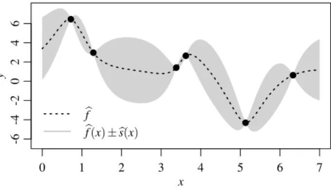
Notice that kriging uses interpolation so that ˆf(xi) = yi and ˆs2(xi) =0,
i=1, . . . ,n. A graphical illustration of the kriging situation can be seen in Fig. 4 showing the prediction ˆf(x) together with the grey uncertainty region
ˆ
f(x)±s(ˆ x).
2.3 Next Design Point
In step 3, the surrogate function based prediction and its uncertainty are con-structed to select the next point for the evaluation. This is realized by the opti-mization of an infill criterion using information of the current model balancing between regions of low mean prediction (exploitation) and of high standard error (exploration). The most typical criterion for the choice of the next design
0 1 2 3 4 5 6 7 x -6 -4 -2 0 2 4 6 y b f b f(x)±bs(x)
Fig. 4 Surrogate function with design points; predicted uncertainty region in grey.
point is the maximization of theexpected improvement conditionally on the observations, as explained now.
Let ˆfn(x)be the surrogate prediction and ˆs2n(x) the prediction uncertainty
based on the firstnevaluations of f. By construction, the estimated surrogate function ˆg(x)follows a normal distribution: ˆg(x)∼N (fˆn(x),sˆ2n(x)). Letφgbe
the corresponding probability density function andΦgthe cumulative
distribu-tion funcdistribu-tion.
Let the actual best value beymin= min
i=1,...,nyi=i=min1,...,nf(xi).For a pointxand
the estimated surrogate g(ˆ x) an improvement is then given by: In(x) =max(ymin−g(ˆ x),0).SinceIn(x) is stochastic, consider the expected
improvement
ei(x) =E(In(x)) =
Z +∞
−∞
max(ymin−y,0)φg(y)dy
=yminΦg(ymin)−E(g(ˆ x)|g(ˆ x)≤ymin)Φg(ymin)
= (ymin−fˆn(x))Φ ymin−fˆn(x) ˆ sn(x) +sˆn(x)φ ymin−fˆn(x) ˆ sn(x) , if ˆsn(x)>0,andE(In(x)) =0 otherwise,
where φ(y) andΦ(y) are the density function and the distribution function
of standard normal distribution. The next point for evaluation is then defined as: xn+1=arg maxx∈ΩE(In(x)). In order to identify this point, the expected improvement has to be optimized numerically, by means of an Evolutionary Algorithm (EA) (see, e.g., Simon (2013)), as originally, or, e.g., by the search method introduced in Sect. 3.3.
2.4 Iteration
In step 4 of the EGO procedure, the objective function is calculated in the new design point. Then, the next iteration step is initiated.
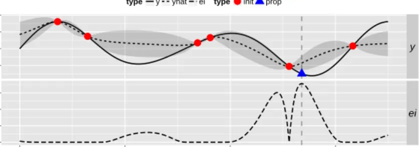
Example 4 (Example 1 cont.).In our example, let us now look at the iterations generating the next design points after the initial design of 6 random points. In Figs. 5 and 6, iterations 1,2,7,10 are visualized. For each iteration the graphic shows in the upper part the original function (solid line) and its approximation
ˆ
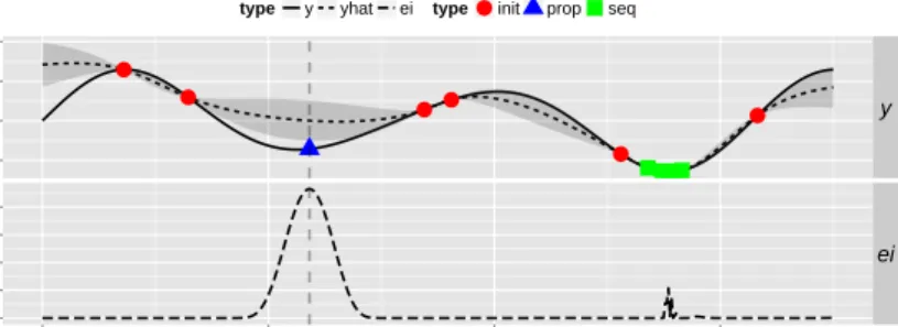
f(x)(dashed line) together with its uncertainty region±s(x)ˆ (grey) and in the lower part the expected improvementei(x). In iteration 1, corresponding to the first new design point, a point near the present minimum is selected (red triangle). This is also true for iteration 2. Thisexploitationof the same region continues up to iteration 6, whereas in iteration 7 a point far off of this region is selected, leading to anexplorationfor other minima. It is this property that enables the method to leave local minima and find global ones. In iteration 10 the search is stopped since also the competing ’classical’ method was based on abudgetof overall 16 design points.
The true optimal setting isxopt≈5.549. With the classical regression model
of order 8, the best evaluated setting wasx=5.688 with an absolute difference to the optimumxoptof 0.139 and the best predicted setting isx=5.586(0.036).
With our EGO model the best evaluated setting isx=5.550(0.001)and the best predicted setting isx=5.515(0.034)which is even somewhat better than for the ‘classical’ performance.
2.5 Stopping
Finally, we should discuss the problem ‘when to stop iteration?’. Typically, a budget is pre-fixed, i.e., the number of iterations. This might lead to early or late stopping, i.e., to stopping without convergence or to stopping far beyond convergence.
Alternatives can be, e.g., based on expected improvement (Huang et al, 2006). We might stop, ifei(x)is small afterniterations, i.e.,
max
x∈{x1,...xn}
● ● ● ● ● ● −4 0 4 8 0.0 0.1 0.2 0.3 y ei 0 2 4 6 x
type y yhat ei type●init prop Iteration 1 ● ● ● ● ● ● −4 0 4 8 0.0 0.1 0.2 y ei 0 2 4 6 x
type y yhat ei type●init prop seq Iteration 2
Fig. 5 Iteration steps 1 and 2 (exploitation); upper parts: objectivef(x)(solid line), predicted objective ˆ
f(x)(dashed line), design points (red dots = initial design, blue triangle = proposed point, green squares = sequential design points after initial design), predicted uncertainty region in grey; lower parts:ei(x).
where ∆s=stopping tolerance, or if relative expected improvement is small,
e.g., if the magnitude ofyis not known: max
x∈{x1,...xn} ei(x)
max{y1, . . . ,yn} −min{y1, . . . ,yn}
<∆r,
where∆r=relative stopping tolerance.
This is the first variation of the standard method we consider in this paper. In the next section, we will discuss other variations.
● ● ● ● ● ● −5 0 5 10 0.000 0.001 0.002 0.003 0.004 y ei 0 2 4 6 x
type y yhat ei type●init prop seq Iteration 7 ● ● ● ● ● ● −5 0 5 10 0.00000 0.00005 0.00010 0.00015 0.00020 y ei 0 2 4 6 x
type y yhat ei type●init prop seq Iteration 10
Fig. 6 Iteration steps 7 (exploration) and 10 (last additional point before stopping); upper parts: objectivef(x)(solid line), predicted objective ˆf(x)(dashed line), design points (red dots = initial design, blue triangle = proposed point, green squares = sequential design points after initial design), predicted uncertainty region in grey; lower parts:ei(x).
3 Variations
Let us now consider variations of the EGO method, particularly for surrogate modeling and the infill criterion. Moreover, details will be discussed on parts of the method not even mentioned yet, namely on the optimization of the infill criterion, and the handling of categorical features.
3.1 Surrogate Models
The choice of the correlation function is one decisive factor for a kriging model. Alternatives to Matérn 3/2 detailed in Sect. 2.2 are, e.g., linear, exponential,
Gaussian, andMatérn 5/2 correlations functions (Rasmussen and Williams, 2006, p. 79ff.). Note that these functions should be as flexible as possible to be able to model any shape of the data.
There are also correlation functions with more than one unknown param-eter, e.g., one scaling parameterψj for each influencing factor in a product
correlation rule:R(ψ1, . . . ,ψp) =∏pj=1R(ψj)(Sasena, 2002), cp. Sect. 4.3.
Also, the ordinary kriging model is generalized, e.g., to theuniversal kriging model, built by a polynomial instead of a constant trend:
g(x) =
k
∑
j=1
βjhj(x) +Z(x)
with arbitrary functionshj and corresponding coefficientsβj (Sasena, 2002).
However, a constant term is generally sufficient because of the flexibility of the correlation functions.
Another variation is the dropping of the interpolation property of kriging. Instead, the kriging model is modeled to be noisy, leading toaugmented kriging (cp. Huang et al (2006)):g(x) =µ+Z(x)+εwithε∼ i.i.N(0,τ2)assumed to
be stochastically independent ofZ(x). The overall covariance can then be writ-ten as Cov(Z(xi)+εi,Z(xj)+εj) =σ2ρ(xi−xj,ψ)+τ2I(i=j),i,j=1, . . . ,n,
whereI(cond)is the indicator function of conditioncond. Such a model is used in Sect. 4.3.
As a further modeling alternative, we propose the use of a classical quadratic regression model instead of a kriging model. Then, variation is mainly modeled explicitly as a function of x: g(xi) =β0+∑pj=1βjxi j+∑pj=1∑kp>jβjkxi jxik+
∑pj=1βj jx2i j+εi, εi ∼ i.i.N (0,σ2). The unknown coefficients βj,βjk,βj j,
j=1, . . . ,p,k> j, and σ2 are estimated by means of least squares.
Predic-tion is then given by ˆf(x) =βˆ0+∑pj=1βˆjxj+∑ p j=1∑
p
k>jβˆjkxjxk+∑pj=1βˆj jx2j
and prediction variance by ˆs2(x) =σˆ2(1+xT(XTnXn)−1x). Note that this leads
to smoothing, not to interpolation. Further note the relationship to the universal kriging model (see above), where thehj(x)stand for the linear, interaction, and
quadratic terms. In universal kriging, for the model residuals a quite general correlation matrix is assumed. In the regression model, the errors are assumed independent, instead. This model is compared to the standard procedure in Sect. 4.1.
3.2 Infill Criteria
In case of the augmented kriging model the expected improvement criterion is extended to theAugmented Expected Improvement aei(x)(cp. Huang et al (2006)): aei(x) = (T−fˆn(x))Φ T−fˆn(x) ˆ sn(x) +sˆn(x)φ T−fˆn(x) ˆ sn(x) · (1−p τˆ ˆ sn(x)2+τˆ2 ),whereT = fˆn(x∗), x∗=arg min x ( ˆ fn(x) +κsˆn(x)),κ=1,typically.
Note thatτ2is the variance of the error termεin the augmented kriging model.
The term (1−√ τˆ
ˆ
sn(x)2+τˆ2) is interpreted as a multiplicative penalty term for
the expected improvement caused by the extra error termε in the augmented
model. Forτ=0, the penalty term is 1 (no penalty). The biggerτis, the smaller is the penalty term and the smaller isaei(x).
Besides the expected improvement, there are other proposals for infill criteria. The most popular alternative is to minimize thelower confidence bound lcb(x) = fˆn(x)−κsˆn(x)with a fixedκ>0 (Cox and John, 1997).
3.3 Search Methods
The optimization of the infill criterion is typically implemented as an approx-imative search. In our group, we proposefocus searchas a global-local opti-mization of the infill criterion to find the next pointxn+1to be evaluated by the
objective black box function f. Focus search will repeatedly start with a coarse LHD with a sequence of refinements near the found optima. The search can be implemented as shown in Algorithm 1.
3.4 Categorical Attributes
One of the disadvantages of standard kriging is its limitation to numerical influential parameters. However, there are extensions to categorical attributes.
Algorithm 1Focus Search
Global search: Repeat fors=1, . . . ,S(e.g.,S=10) Local search: Repeat forj=1, . . . ,J(e.g.,J=5)
(a) Sample LHD:Dj⊂Ωj(Ω1=Ω) (b) Infill Criterion, e.g.,lcbwithκ=1:
Candidate pointx∗j=arg minx∈Dj[fˆ(x)−sˆ(x)]
(c) Reduce parameter space:Ωj+1⊂Ωjaroundx∗j
Local candidates: D∗s={x∗1, . . . ,x∗J}andxs=arg minx∈D∗s[fˆ(x)−sˆ(x)]best point
Global candidates: Let D∗ = {x1, . . . ,xS} be the global candidate set, then xn+1 :=
argminx∈D∗[fˆ(x)−sˆ(x)]is the best point to be evaluated next
In the literature, most of the time, extensions of the covariance function to qualitative variables are proposed (see, e.g., Qian et al (2008)). In contrast, we propose two very simple methods, indicated below:
Naïve kriging: Categorical attributes are handled as numerical ones by as-signing an integer value to each level. This method is easy to implement, but the order of the levels and the distance between levels are typically artificial. Dummy kriging: Dummy variables are built for each categorical attribute, e.g., for possible levelsA,B,Cof attributexwe takexA=I[x=A],xB=I[x=B], xC=I[x=C]. This method is statistically more correct, but time consuming if categorical attributes have a large number of levels.
For an application, where these two methods are compared, see Sect. 4.2.
4 Applications
4.1 Parameter Tuning
The first application will be parameter tuning for Support Vector Machine (SVM) classification (Schölkopf and Smola, 2002).
To illustrate the method, we use 5 publicly available classification bench-mark problems fromOpenML(Vanschoren et al, 2014) (www.openml.org) characterized in Table 1. We would like to compare kriging modeling with regression modeling in EGO as well aseiandlcbas infill criteria. As the ob-jective f(cost,γ,ε)we use the error rate of the nonlinear SVM classifier using
theRadial Basis Function(RBF) kernel (as provided in the library LIBSVM, cp. Chang and Lin (2011)) with thep=3 parameterscost, penalizing errors,γ
Table 1 Data sets used in SVM parameter tuning characterized by the number of observations (obs), the number of variables (m), and the best accuracy reached with the focused grid search for the shown parameter settings.
Dataset obs m Best Accuracycost γ ε
spambase 4 601 58 0.059 1.38e+03 2.06e-04 1.28e-04 wilt 4 829 6 0.007 2.34e+03 2.19e-02 3.29e-04 ada_agnostic 4 562 49 0.182 1.56e+00 3.31e-05 1.98e-01 eeg-eye-state 14 980 15 0.095 2.37e+04 7.23e-01 8.73e-02 MagicTelescope 19 020 12 0.001 1.71e+04 5.52e-02 1.94e-04
in the RBF kernel, andε in the loss function. In this way, optimal tuning of the
SVM parameters is realized. ● ● ● ● ● ● ● ● ● ● ● ● ● ● ● ● ● ● ● ● ● ● ● ● ● ● ● ● ● ● ● ● ● ● ● ● ● ● ● ● ● ● ● ● ● ● ● ● ● ● ● ● ● ● ● ● ● ● ● ● ● ● ● ● ● ● ● ● ● ● ● ● ● ● ● ● ● ● ● ● ● ● ● ● ● ● ● ● ● ● ● ● ● ● ● ● ● ● ● ● ● ● ● ● ● ● ● ● ● ● ● ● ● ● ● ● ● ● ● ● ● ● ● ● ● ● ● ● ● ● ● ● ● ● ● ● ● ● ● ● ● ● ● ● ● ● ● ● ● ● ● ● ● ● ● ● ● ● ● ● ● ● ● ● ● ● ● ● ● ● ● ● ● ● ● ● ● ● ● ● ● ● ● ● ● ● ● ● ● ● ● ● ● ● ● ● ● ● ● ● ● ● ● ● ● ● ● ● ● ● ● ● ● ● ● ● ● ● ● ● ● ● ● ● ● ● ● ● ● ● ● ● ● ● ● ● ● ● ● ● ● ● ● ● ● ●●●●●●● ●●●●●●● ●●●●●●● ●●●●●●● ●●●●●●● ●●●●●●● ●●●●●●● ●●●●●●● ●●●●●●● ●●●●●●● ●●●●●●● ●●●●●●● ●●●●●●● ●●●●●●● ●●●●●●● ●●●●●●● ●●●●●●● ●●● ●●● ●●●●●●● ●●●●●●● ●●●●●●● ●●●●●●● ●●●●●●● ●●●●●●● ●●●●●●● ●●●●●●● ●●●●●●● ●●●●●●● ●●●●●●● ●●●●●●● ●●●●●●● ●●●●●●● ●●●●●●● ●●●●●●● ●●●●●●● ●●●●●●● ●●●●●●● ●●●●●●● ●●●●●●● ●●●●●●● ●●●●●●● ●●●●●●● ●●●●●●● ●●●●●●● ●●●●●●● ●●●●●●● ●●●●●●● ●●●●●●● ●●●●●●● ●●●●●●● ●●●●●●● ●●●●●●● ●●●●●● ●●●●●●● ●●●●●●● ●●●●●●● ●●●●●●● ●●●●●●● ●●●●●●● ●●●●●●● ●●●●●●● ●●●●●●● ●●●●●●● ●●●●●●● ●●●●●●● ●●●●●●● ●●●●●●● ●●●●●●● ●●●●●●● ●●●●●●●●●●●●●●●●●●●●●●●●●●●●●●●●●●●●●●●●●●●●●●●●●●●●●●●●●●●●●●●●●●●●●●●●●●●●●●●●●●●●●●●●●●●●●●●●●●●●●●●●●●●●●●●●●●●●●●●●●●●●●●●●●●●●●●●●●●●●●●●●●●●●●●●●●●●●●●●●●●●●●●●●●●●●●●●●●●●●●●●●●●●●●●●●●●●●●●●●●●●●●●●●●●●●●●●●●●●●●●●●●●●●●●●●●●●●●●●●●●●●●●●●●●●
1e−04 1e−02 1e+00 1e+02 1e+04
1e−04 1e−02 1e+00 1e+02 1e+04 cost γ
Fig. 7 Focused Grid Search for the 2 SVM para-meterscostandγ. First, the focus is on the bottom right corner (blue region). Then, the focus is shifted somewhat to the left (light-blue region).
Since the ground truth is not avail-able, we apply a somewhat naïve ap-proach for generating a near opti-mum of the objective being the ac-curacy of the model. We use a Fo-cused Grid Search over the 3 para-meterscost,γ,ε. We considercost∈
2[−15,15],γ ∈2[−15,15], ε ∈ 2[−13,−1],
vary all parameters on a logarithmic scale, and use 7·7·5=245 points, equidistant in each dimension, as the starting grid. We use J = 4 Focus Search iterations (and S = 1, i.e., only one fixed starting grid) (cp. Sect. 3.3) leading to 980 function evaluations. See Fig. 7 for an illustration.
The performance corresponding to a found(cost,γ,ε)setting is assessed via a 2:1 train-test-split. The accuracy of the optimum found by the Focused Grid Search is taken as the ground truth for a comparison with the best accuracies found by the different versions of the EGO procedure. The results of the Focused Grid Search can be found in Table 1.
For the evaluation of the EGO procedures, we count the number of function evaluations until EGO reaches the same performance as the grid search. We start with a random LHS with 4p=12 points (in order to make sure that all parameters are estimable with quadratic regression), vary the infill criterion
(eiandlcb) and the surrogate model (kriging and quadratic regression), and consider 5 replications. We say that EGO failed if the solution was not reached after 500 iterations since we expect that one EGO step is roughly a factor of two slower than one pure function evaluation.
In Table 2, the iteration characteristics of EGO are reported for the different data sets and method variants, namely the median of the iteration counts of successful EGO runs and the number of successful EGO replications in brackets. In Table 3, the differences of the best optimizations runs to the grid search performance are reported.
Table 2 Median iteration counts of SVM parameter tuning (number of successful KM or QM replica-tions), KM = Kriging Model, QM = Quadratic regression Model
Dataset ei + KM lcb + KM ei + QM lcb + QM spambase 30 (5) 48 (5) - (0) - (0) wilt 18 (5) 15 (5) 17 (5) 18 (5) ada_agnostic 35 (1) 80 (3) - (0) - (0) eeg-eye-state 45 (5) 43 (5) 84 (2) 260 (2) MagicTelescope 29 (5) 39 (5) 16 (1) 15 (2)
Table 3 Differences of the best optimization results to the grid search optimum, KM = Kriging Model, QM = Quadratic regression Model
Dataset Grid Search ei + KM lcb + KM ei + QM lcb + QM spambase 0.059 -6.52e-04 -6.52e-04 +6.52e-04 +6.52e+04 wilt 0.007 -6.20e-04 -6.20e-04 -6.20e-04 -6.20e-04 ada_agnostic 0.182 0 -6.57e-04 +1.31e-03 +1.31e-03 eeg-eye-state 0.095 -1.60e-03 -4.00e-04 -2.00e-04 +2.00e-04
MagicTelescope 0.001 0 -1.58e-04 0 0
Overall, the results can be interpreted as follows. When comparing EGO and Grid Search, EGO wins by a clear margin. If EGO is able to find the optimal target function value, it is around 20 times faster. If EGO does not reach the optimal target value, it is only slightly off-target.
When comparingeiandlcb, no real winner can be identified. There are only small differences, each method is better in some cases. However,lcb could be preferable since this criterion does not rely on the validity of the normal distribution.
When comparing the results of regression and kriging, kriging is distinctly superior. Regression fails very often (only 17 successful replications overall in
contrast to 44 for kriging). Moreover, regression is not as flexible as kriging. Only if the optimum of the quadratic model is near to the real optimum, the real optimum is reliably found (e.g., for the data set “wilt”). Larger initial designs or the concentration on the best or the newest observations might help regression. This will be studied further.
Let us finish this discussion by a remark on parallel computing. Focused Grid Search can use many nodes in parallel. However, EGO suffers from its iterative behavior, i.e., its evaluation of the 500 points has to be realized one after the other. Therefore, in real time Focused Grid Search was much faster (not in computing time!). A possible way out of this problem is the development of efficient Multi Point Proposals, where multiple proposal points are suggested in parallel (cp. Bischl et al (2014)).
4.2 Onset Detection
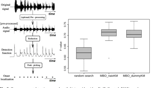
The second application deals with the optimization of music onset detection. In this study, a tone onset is the time point of the beginning of a musical note played by a musical instrument. The ability of the detection of tone onsets depends on the instrument playing the tone, e.g., the beginning of piano tones can be much easier identified than the beginning of flute tones (see Fig. 8).
0 1 2 3 4 time in seconds amplitude −7000 0 7000 0 1 2 3 time in seconds amplitude −5000 0 5000
Fig. 8 Time series of the same music piece played by piano (left) and flute (right); tone beginnings are marked by vertical lines.
The onset detection algorithm we use in this study is specified in Algorithm 2 (cp. Fig. 9 (left)); for more details see Bauer et al (2016).
Algorithm 2Onset detection algorithm
Input: Audio data in WAVE format with sampling rate of 44.1 kHz
1: Windowing: Split signal into small windows (parameters: window size 512−4096 samples and shift to next window (called hop size)(0−90% of the window size))
2: Pre-processing: Pre-process the data (parameters: windowing function (Hanning, Gauss,. . .), spectral filter (yes /no), log-scale (yes /no), and log-parameter (1 – 20))
3: Detection function: Compute in each window an onset detection function (odf) (parameters: odf function (amplitude increase, spectral flux,. . .) and exponential smoothing with a parameter in
[0,1])
4: Peak-picking: Threshold the smoothed odf (parameters: moving function (mean, median,. . .), threshold multiplier (1 – 3), threshold additive term (0 – 10), and threshold time back (0 – 0.5 seconds))
5: Onset localization: Localize the tone onsets (parameters: onset time back (0 – 0.5 seconds), min. distance between onsets (0 – 0.05 seconds), and onset shifting time (−0.01 – 0.02 seconds)) Output: F-value
As the objective, the F-measureF= 2c+f2+c+f− is used, wherec=number
of correct detections, f+=number of false positive detections, and f−= num-ber of false negative detections. We use EGO to optimize F corresponding to the 15 parameters, 10 numerical and 5 categorical, of the onset detection in Algorithm 2, i.e., we optimize f(window size, . . . , onset shifting time) = F(window size, . . . ,onset shifting time).
We use the following EGO settings: kriging with the covariance function Matérn 3/2 as the surrogate model,eias the infill criterion, focus search with S=3,J=5, and size ofDj=10’000 points as the infill optimizer, LHS with
5d =75 points as the initial design, and 20d =300 iterations. Note that 5 categorical parameters have to be optimized. Therefore, we will compare naïve kriging and dummy kriging (cp. Sect. 3.4).
As the validation design, we use 321 hand labeled music data files in WAVE format (IBM and Microsoft, 1991) as the learning data set, 2/3 data for training and 1/3 for testing in the train-test-approach, and 30 replications (subsampling). The idea is to find the best setting of the parameters in Algorithm 2 on the training data and evaluate it on the test data. As the objective, F-values on the test data are used.
● 0.55 0.60 0.65 0.70 0.75 F−v alue
random search MBO_naivKM MBO_dummyKM
Fig. 9 Common onset detection procedure (left) (see Algorithm 2) (Bello et al, 2005); random search compared to EGO with naïve kriging and dummy kriging (right).
The resulting distribution of F-values can be found in Fig. 9 (right). EGO variants clearly dominate random search based on an LHS design of size 25d. Naïve kriging shows slightly better results than dummy kriging.
4.3 Cutting Optimization
The goal of the third application is the optimization of a cutting process with a diamond tipped drill core bit. We start with a single diamond scratch test, want-ing to find settwant-ings of the process and production factors which minimize work to reach a certain drilling depth. For this, we first optimize a simulation model by means of parameter adjustment with EGO, and then optimize the process and production factors using the optimal simulation output (cp. Herbrandt et al (2016)).
In order to optimize a simulation model we first need to observe the real process. For this, we carry out a block design with 60 trials each for the 5 materials cement, basalt, concrete, steel, and reinforced concrete. We base on 5 samples per material. We aim to achieve 80µm total drilling depth. We
compare 4 feed speedνf (mm/min) settings and 4 cutting speedνc (m/min)
same speed settings (νc,νf) are treated in pairs of adjacent radii each. This
leads to minimum 2 replicates per setting (νc,νf) (cp. Fig. 10 for an example).
Overall, we use 5 blocks (samples) with 6 trials (radii) each and speed settings from a full factorial design. The design is D-optimized, twice replicated in (νc,νf). The outputs are the forces (Fx,Fy,Fz)in all 3 dimensions. The normal
force in Fig. 10 corresponds toFz. The sampling rate is 200’000 Hz.
time [s] nor mal f orce [N] 0.0 0.2 0.4 0.6 0.8 0 5 10 15 20 radius mm 20 21
Fig. 10 Time series of normal forces on cement for the speed combinationνc=193.5minm,νf=7mmmin; red: radius = 20 mm, green: radius=21 mm
Let us now optimize a simulation model for the forcesF(r,xxx)with 8 para-metersxxx= (gz,gv,µc,σY c2,τc2,ψc,pc,qc)given as a weighted sum of removed
volumesvand characteristic material valuesz: F(r,xxx) =gz r z(µc,σ 2 Y c,τc2,ψc)v(pc,qc) + gv r v(pc,qc) +ε.
For the model of the removed volumevwe assume that the cutting diamond has the shape of a pyramid and the cutting line has the profile of a triangle. The triangle size depends on the current observation, the cutting depth per revolution, and the stochastic brittleness of the material simulated by a restricted Beta(pc,qc)-distributed deviation from the perfect cutting profile. The removed
volume of one observation is the volume between two consecutive triangles. For the model of the characteristic material valueszwe assume that forces needed to remove material vary over the work piece. The characteristic mate-rial values (e.g. hardness) of the triangle points are sampled from a Gaussian random fieldZ(µc,σY c2 ,τc2,ψc). The material value of one observation is the
As the objective function f(Fz(r,νc,νf),F(r,x))for EGO optimization, we
use the mean deviation between modeled forcesF(r,x)and observed forces Fz(r,νc,νf)corresponding to the three characteristics slope, range, and
spec-trum (Herbrandt et al, 2016). For force modeling, we use the same radii r as for the realization of observed forces. The objective is stochastic because of the stochastic character of the force model. The unknown parameters are
x= (gzgvµcσY c2 τc2ψc pcqc)T of the above force function. So we havep=8
unknown parameters. The initial design is taken to be a random Latin hyper-cube withn0=10p=80 points, the number of iterations is set to be 720. This
leads to a total number of function evaluations of 100p=800. As the surro-gate function we use the augmented (noisy) kriging model (cp. Sect. 3.1), as the infill criterion the augmented expected improvement (cp. Sect. 3.2). Please compare the pseudocode in Algorithm 3. Please distinguish the Gaussian ran-dom fieldZ(µc,σY c2 ,τc2,ψc) for the characteristic material values (see above)
from the Gaussian random field with parametersθ = µ σ2τ2ψ1 . . .ψ8
T used in kriging. Model parameters are optimized individually for each of the 16 speed combinations (νc,νf) and each material (in our illustrations we take
cement).
Algorithm 3Optimization of force model Input: Observed normal forcesFzwith speed settings νc,νf
Initial Design:
(a) Sample 80 parameter settings x1, . . . ,x80∈R8 from a random Latin hypercube,xi=
(gzigviµciσY ci2 τci2ψcipciqci)T
(b) Evaluate objective function f inx1, . . . ,x80: f Fz r,νc,νf,F(r,xi)=yi,i=1, . . . ,80, where f is the mean deviation between modeled and observed forces corresponding to the three characteristics slope, range, and spectrum
EGO: Repeat fori=80, . . . ,799 Surrogate Function:
(1) Estimate the augmented kriging parametersθ= µ σ2τ2ψ1. . .ψ8(see Sect. 3.1), where theψjare the Matérn parameters for the individual dimensions
(2) Determine the augmented kriging prediction ˆfi θˆconditional ony1, . . . ,yi (3) Determine the augmented kriging uncertainty ˆs2
i θˆ
conditional ony1, . . . ,yi
Infill Criterion: Maximize the augmented expected improvementaei(x)in Sect. 3.2 with the focus search in Algorithm 1:xi+1=arg maxx∈Ωaei(x)
Evaluation: Evaluate objective functionfinxi+1
Output: Optimal force model parametersx?= gz∗gv∗µ
c∗σY c2∗τc2∗ψc∗p∗cq∗c
Looking at the optimization results, the best fit is achieved for (νc,νf) =
(270, 7), the worst fit for (νc,νf) = (270, 9.5) (cp. Table 4). The goodness of fit
depends on the similarity of ‘repetitions’. The iteration number corresponding to the optimal parameter setting is typically lower than the budget of 800 iter-ations. See Fig. 11 for an example, where near optimal settings were already found very early, i.e., after less than 250 iterations. For each optimization we obtain the values of the evaluated objective function y1, . . . ,y800 and the
op-timal parameter vectorx∗ = (gz∗gv∗µc∗σY c2
∗
τc2
∗
ψ∗p∗cq∗c)T. Since the best
model is stochastic, we only check how well an observed realization with this speed combination fits into the area of simulated realizations. See Fig. 12 for an example.
Table 4 Optimal valuesyminof objective for the different combinations (νc,νf) and corresponding iteration numbersnmin
νc 40.5 40.5 40.5 40.5 117 117 117 117 193.5 193.5 193.5 193.5 270 270 270 270 νf 2 4.5 7 9.5 2 4.5 7 9.5 2 4.5 7 9.5 2 4.5 7 9.5 ymin 3.25 3.04 5.64 4.32 1.49 3.81 7.08 4.41 1.66 3.73 1.75 6.95 2.09 4.75 1.45 7.61 nmin 328 621 682 299 800 490 427 434 731 171 452 423 122 755 672 261 0 10 20 30 40 50 y
number of evaluated points
y 200 400 600 nmin 800 | {z } initial design ymin 2 2.5
Fig. 11 Optimization path for speed combinationνc=270minm andνf=7 mmmin; the end of the initial design is indicated by a vertical line; the minimumyminis reached for iteration numbernmin. The lower part is a zoom-in of the upper part.
Based on the optimal force models we now would like to optimize the pro-cess and production factors. We use the modeled forces to predict a speed-combination with minimal workWA needed to drill a desired depthA(here:
Fig. 12 Time series of 50 realizations of the force model with optimal parameter setting (blue) and observed force (black) for the speed combinationνc=270minm andνf=7 mmminon the radius 18mm.
(a) (b)
Fig. 13(a) Realizations of the force model (blue), observed force (black), expected modeled forces F(s)(red line), and the resulting workWA(red hatched) to reach a total depth ofA=0.07mmwith
νc,νf,r= 270minm,7 mmmin,18mm; (b) Surface of the generalized linear model of the resulting work, split by the radiir=16mm(yellow), ...,r=27mm(violet).
A=0.07mm):WA=
RsA
0 F(s)ds, wheresA=sA(r) =total distance until
reach-ing depthA(mm),F(s) =expected modeled forces for distances. For an exam-ple, see Fig. 13(a).
The independent variables areνc,νf,r. We use aGeneralized Linear Model
(GLM) (Nelder and Wedderburn, 1972) with Gamma distributed error, log link, and with up to cubic terms and all interactions. We apply backwards variable selection based on the Akaike Information Criterion (AIC) (Akaike, 1974).
The resulting model fit is nearly perfect (goodness of fit: pseudoR2=0.998). This model results in optimal speeds which are nearly the same for each ra-dius:(νc,νf)≈(40.5,8.75). For the dependence of work on the speeds(νc,νf)
please compare Fig. 13(b). The independence of optimal speeds(νc,νf)on the
radiusr is what we hoped for. Too small values ofνf lead to higher friction
and lower material removal, i.e., to higher total work. Too highνf values cause
higher total work due to very high material removal rates.
5 Conclusions
EGO is especially appropriate for the optimization of expensive black box func-tions. If evaluation cost is low, cost of surrogate model estimation can exceed the cost for objective function evaluation. EGO with kriging not only focuses on finding the optimum but the exploration during this process also leads to a good model fit over the whole parameter region. Variations are diverse, concerning, e.g. the covariance structure, the infill criterion, the search structure, categori-cal factors, noise, the regression model, etc. We introduced some new variants like regression as a modeling alternative to kriging and two simple methods for the handling of categorical variables, and we discussed focus search for the optimization of the infill criterion. Applications are numerous. We looked at parameter tuning and optimization in practice. The R package mlrMBO, devel-oped in our group (Bischl et al, 2015), provides all the described methods and further features like, e.g. optimization with more than one objective function.
Acknowledgements
We acknowledge support by the German Research Foundation (DFG) within the Collaborative Research Center SFB 823Statistical modeling of nonlinear dynamic processes, Projects B3, B4, and C2.
References
Adler RJ, Taylor JE (2007) Random fields and geometry. Springer Monographs in Mathematics, Springer-Verlag, New York, DOI 10.1007/ 978-0-387-48116-6
Akaike H (1974) A new look at the statistical model identification. IEEE Transactions on Automatic Control 19(6):716–723, DOI 10.1109/TAC.1974. 1100705
Bauer N, Friedrichs K, Bischl B, Weihs C (2016) Fast Model Based Optimiza-tion of Tone Onset DetecOptimiza-tion by Instance Sampling, Springer InternaOptimiza-tional Publishing, Cham, pp 461–472. DOI 10.1007/978-3-319-25226-1_39 Bello JP, Daudet L, Abdallah S, Duxbury C, Davies M, Sandler MB (2005) A
tutorial on onset detection in music signals. IEEE Transactions on Speech and Audio Processing 13(5):1035–1047, DOI 10.1109/TSA.2005.851998 Bischl B, Wessing S, Bauer N, Friedrichs K, Weihs C (2014) MOI-MBO:
Mul-tiobjective infill for parallel model-based optimization. In: Pardalos PM, Re-sende MG, Vogiatzis C, Walteros JL (eds) Learning and Intelligent Optimiza-tion, Springer International Publishing, Switzerland, Lecture Notes in Com-puter Science, vol 8426, pp 173–186, DOI 10.1007/978-3-319-09584-4_17 Bischl B, Bossek J, Richter J, Horn D, Lang M (2015) mlrMBO: mlr: Model-based optimization. https://github.com/berndbischl/mlrMBO, R package ver-sion 1.0
Chang CC, Lin CJ (2011) Libsvm: A library for support vector machines. ACM Transactions on Intelligent Systems and Technology 2(3):27:1–27:27, DOI 10.1145/1961189.1961199
Cioppa TM, Lucas TW (2007) Efficient nearly orthogonal and space-filling latin hypercubes. Technometrics 49(1):45–55, DOI 10.1198/ 004017006000000453
Cox DD, John S (1997) SDO: A statistical method for global optimization. In: Alexandrov M, Hussaini M (eds) Multidisciplinary Design Optimization: State of the Art, Society of Industrial and Applied Mathematics and Applied Mathematics (SIAM), Philadelphia, pp 315–329
Cressie N (1988) Spatial prediction and ordinary kriging. Mathematical Geol-ogy 20(4):405–421, DOI 10.1007/BF00892986
Herbrandt S, Ligges U, Ferreira M, Kansteiner D, Biermann D, Tillmann W, Weihs C (2016) Model based optimization of a statistical simulation model
for single diamond grinding. Computational Statistics, to appear DOI 10. 1007/s00180-016-0669-z
Huang D, Allen TT, Notz WI, Zheng N (2006) Global optimization of stochastic black-box systems via sequential kriging meta-models. Journal of Global Optimization 34:441–466, DOI 10.1007/s10898-005-2454-3
IBM, Microsoft (1991) Multimedia programming interface and data
specifica-tions 1.0. URLhttp://www-mmsp.ece.mcgill.ca/documents/
audioformats/wave/wave.html
Jones DR, Schonlau M, Welch WJ (1998) Efficient global optimization of ex-pensive black-box functions. Journal of Global Optimization 13:455–492, DOI 10.1023/A:1008306431147
Matérn B (1986) Spatial variation, Springer Lecture Notes in Statistics, vol 36. Springer-Verlag, New York
McKay MD, Beckman RJ, Conover WJ (1979) A comparison of three meth-ods for selecting values of input variables in the analysis of output from a computer code. Technometrics 21(1):239–245, DOI 10.2307/1268522 Mood AM (1950) Introduction to the Theory of Statistics. McGraw-Hill, New
York
Myers RH, Montgomery DC, Anderson-Cook CM (2009) Response Surface Methodology. Wiley. Hoboken, New Jersey
Nelder J, Wedderburn R (1972) Generalized linear models. Journal of the Royal Statistical Society Series A 135(3):370–384, DOI: 10.2307/2344614 Qian PZG, Wu H, Wu CFJ (2008) Gaussian process models for computer
ex-periments with qualitative and quantitative factors. Technometrics 50(3):383– 396, DOI 10.1198/004017008000000262
Rasmussen CE, Williams CKI (2006) Gaussian processes for machine learning. The MIT Press, Cambridge, Massachusetts
Sasena MJ (2002) Flexibility and efficiency enhancements for constrained global design optimization with kriging approximations. PhD thesis, General Motors
Schölkopf B, Smola AJ (2002) Learning with Kernels: Support Vector Ma-chines, Regularization, Optimization, and Beyond. MIT Press, Cambridge, Massachusetts
Simon D (2013) Evolutionary Optimization Algorithms. Wiley, Hoboken, New Jersey
Vanschoren J, van Rijn JN, Bischl B, Torgo L (2014) OpenML: Networked science in machine learning. SIGKDD Explor Newsl 15(2):49–60, DOI 10.1145/2641190.2641198