Department of electrical engineering and computer science
Geometric optimization algorithms
for linear regression on fixed-rank matrices
PhD thesis of Gilles Meyer
Advisor: Prof. Rodolphe Sepulchre Co-advisor: Dr. Silvère Bonnabel
June 2011
Jury members:
L. Wehenkel (President) Professor, University of Liège R. Sepulchre (Advisor) Professor, University of Liège S. Bonnabel (Co-advisor) Maître-assistant, Mines ParisTech
P. Geurts FNRS research associate, University of Liège
P.-A. Absil Associate professor, Université Catholique de Louvain F. Bach INRIA researcher, Ecole Normale Supérieure, Paris I. Dhillon Professor, University of Texas, Austin
Nowadays, large and rapidly evolving data sets are commonly encountered in many modern applications. Efficiently mining and exploiting these data sets generally results in the extraction of valuable information and therefore appears as an important challenge in various domains including network security, computer vision, internet search engines, bioinformatics, marketing systems, online advertisement, social networks, just to name a few.
The rapid development of these modern computer science applications sustains an ever-increasing demand for efficient machine learning algorithms that can cope with large-scale prob-lems, characterized by a large number of samples and a large number of variables.
The research reported in the present thesis is devoted to the design of efficient machine learning algorithms for large-scale problems. Specifically, we adopt a geometric optimization viewpoint to address the problem of linear regression in nonlinear and high-dimensional matrix search spaces. Our purpose is to efficiently exploit the geometric structure of the search space in the design of scalable linear regression algorithms.
Our search space of main interest will be the set of low-rank matrices. Learning a low-rank matrix is a typical approach to cope with high-dimensional problems. The low-rank constraint is expected to force the learning algorithm to capture a limited number of dominant factors that mostly influence the sought solution. We consider both the learning of a fixed-rank symmetric positive semidefinite matrix and of a fixed-rank non-symmetric matrix.
A first contribution of the thesis is to show that many modern machine learning problems can be formulated as linear regression problems on the set of fixed-rank matrices. For example, the learning of a low-rank distance, low-rank matrix completion and the learning on data pairs are cast into the considered linear regression framework. For these problems, the low-rank constraint is either part of the original problem formulation or is a sound approximation that significantly reduces the original problem size and complexity, resulting in a dramatic decrease in the computational complexity of algorithms.
Our main contribution is the development of novel efficient algorithms for learning a linear regression model parameterized by a fixed-rank matrix. The resulting algorithms preserve the underlying geometric structure of the problem, scale to high-dimensional problems, enjoy local convergence properties and confer a geometric basis to recent contributions on learning fixed-rank matrices. We thereby show that the considered geometric optimization framework offers a solid and versatile framework for the design of rank-constrained machine learning algorithms.
The efficiency of the proposed algorithms is illustrated on several machine learning applica-tions. Numerical experiments suggest that the proposed algorithms compete favorably with the state-of-the-art in terms of achieved performance and required computational time.
A l’heure actuelle, des bases de données de grande taille et soumises à des modifications régulières sont rencontrées dans la plupart des applications modernes. Une exploitation efficace de ces données constitue un enjeu essentiel dans de nombreux domaines d’activités tels que la sécurité des réseaux, la vision par ordinateur, les moteurs de recherche internet, la bioinformatique, les systèmes de marketing, la publicité en ligne ou encore les réseaux sociaux.
Le développement rapide de ces applications entretient une demande sans cesse croissante pour des algorithmes d’apprentissage automatique efficaces, capables de traiter des problèmes de grande taille en termes du nombre d’échantillons et du nombre de variables.
La recherche présentée dans cette thèse de doctorat est dédiée à l’élaboration d’algorithmes d’apprentissage automatique capables de traiter efficacement des problèmes de grande taille. Plus spécifiquement, nous adoptons un cadre géométrique d’optimisation pour aborder le prob-lème de la regression linéaire dans des espaces de recherche non linéaires et de grande dimension. L’approche proposée repose sur une exploitation adéquate de la géométrie du problème pour élaborer de nouveaux algorithmes d’optimisation efficaces appliqués à la régression linéaire.
L’espace de recherche sur lequel porte principalement notre intérêt est l’ensemble des matrices réelles de rang faible et fixé. L’apprentissage d’une matrice de rang faible est une approche typique pour aborder des problèmes de grande dimension. La contrainte de rang faible tend à forcer l’algorithme d’apprentissage à capturer un nombre limité de facteurs dominants qui influences la solution recherchée. Nous abordons l’apprentissage des matrices réelles symétriques semidefinies positives de rang fixé puis nous généralisons les résultats obtenus aux matrices réelles non symétriques de rang fixé.
Une première contribution de cette thèse de doctorat est de montrer que de nombreux prob-lèmes récents en apprentissage automatique peuvent être formulés comme un problème de régres-sion linéaire sur l’espace des matrices de rang fixé. Par exemple, l’apprentissage d’une mesure de distance, la complétion de matrices, l’apprentissage sur des paires de données sont des prob-lèmes qui se formulent naturellement dans le cadre de travail considéré. Pour ces probprob-lèmes, la contrainte de rang fixé apparaît naturellement, soit parce qu’elle fait partie de la formulation originale du problème, soit parce qu’elle permet une approximation raisonable de la solution, tout en réduisant significativement la taille et la complexité du problème original et la complexité des algorithmes.
Notre contribution principale est la conception de nouveaux algorithmes efficaces pour ap-prendre un modèle de régression linaire paramétré par une matrice de rang fixé. Les algorithmes résultants préservent la géométrie du problème, sont applicables à des problèmes de grande di-mension, présentent des propriétés de convergence locales et confèrent une base géométrique à des contributions récentes sur l’apprentissage des matrices de rang fixé. Nous montrons de ce fait que les techniques d’optimisation considérées offrent un cadre de travail solide et flexible pour la conception de nouveaux algorithmes pour apprendre une matrices de rang fixé.
L’efficacité des algorithmes proposés est illustrée sur plusieurs problèmes d’aprentissage au-tomatique, dont l’apprentissage d’une distance, la complétion de matrices et l’apprentissage sur des paires de données. Les simulations numériques effectuées suggèrent que les algorithmes pro-posés rivalisent favorablement avec l’état de l’art, à la fois en terme des performances obtenues et du temps de calcul requis.
Completing this thesis has been a rich, positive and often overwhelming personal experience. However, the work that I have carried out during the last four years would have been impossible without the help and support from many people to whom I would like to express my sincere appreciation.
First and foremost, my hearty thanks go to my advisor, Rodolphe Sepulchre, for his ever pertinent guidance and unconditionally enthusiastic support. I am very grateful to Rodolphe for his precious advice and for sharing with me his expertise and enthusiasm. Rodolphe has been for me a marvelous consultant and an outstanding project manager; who always succeeded in providing me optimism and motivation, especially when I needed it the most.
I warmly thank my closest collaborators Silvère Bonnabel (co-advisor of this thesis), Michel Journée and Bamdev Mishra who directly contributed to the present work. They have been of great help both scientifically and personally. Special thanks go to Silvère and Michel for coaching me with patience and talent during the beginning of my thesis.
I also owe warm thanks to Pierre Geurts and Alain Sarlette for inspiring research discussions and precious advice on subjects related to the present work.
These four years spent at Montefiore Institute have been extremely pleasant for many reasons. One of the most important reasons is great friends and colleagues from the research unit, past and present. I enjoyed very much working and exchanging with them during the last four years. Special thanks go to the “Coffee break” group for entertaining breaks and lunches.
I thank the administrative staff of the Montefiore Institute, and in particular Charline for her constant kindness and precious help.
I would also like to express my genuine appreciation to all members of the jury, Pierre-Antoine Absil, Francis Bach, Silvère Bonnabel, Inderjit Dhillon, Pierre Geurts, Rodolphe Sepulchre and Louis Wehenkel for devoting time and interest to the reading and evaluation of this manuscript. I gratefully acknowledge the financial support from the Belgian National Fund for Scientific Research (FNRS) as well as from the Belgian Network DYSCO (Dynamical Systems, Control, and Optimization), funded by the Interuniversity Attraction Poles Programme, initiated by the Belgian State, Science Policy Office.
Last but not least, I want to express my deepest gratitude to my family and friends for their constant support and for helping me disconnect from research when needed. Super special thanks to my wonderful and lovely wife Estelle, who has been of invaluable patience and support.
1 Introduction 1
1.1 Research context . . . 2
1.2 Contributions . . . 4
1.3 Outline . . . 6
2 Linear regression on nonlinear spaces 9 2.1 Motivation and applications . . . 9
2.2 Problem formulation . . . 14
2.3 Gradient based learning . . . 14
2.4 Linear regression in vector search spaces . . . 15
2.5 Linear regression in matrix search spaces . . . 17
3 A geometric optimization framework for regression 25 3.1 Optimization on Riemannian matrix manifolds . . . 25
3.2 Tangent space of an embedded submanifold . . . 26
3.3 Tangent space of a quotient manifold . . . 27
3.4 Line-search algorithms on matrix manifolds . . . 29
3.5 Trust-region algorithms on matrix manifolds . . . 34
4 Regression on fixed-rank symmetric positive semidefinite matrices 37 4.1 Introduction . . . 37
4.2 Regression on the cone of positive definite matrices . . . 39
4.3 From positive definite to fixed-rank positive semidefinite matrices . . . 41
4.4 Algorithms . . . 43
4.5 Discussion . . . 46
4.6 Experiments . . . 48
4.7 Conclusion . . . 57
5 Regression on fixed-rank non-symmetric matrices 59 5.1 Introduction . . . 59
5.2 Quotient geometries of fixed-rank matrix factorizations . . . 60
5.3 Geometry of algorithms using a fixed-rank factorization . . . 61
5.4 Algorithms for regression on fixed-rank non-symmetric matrices . . . 63
5.5 Experiments . . . 70
5.6 Conclusion . . . 72
6 From first-order to second-order optimization algorithms 73 6.1 Introduction . . . 73
6.2 Formulas for the Riemannian connection . . . 74
6.3 Computing the Riemannian Hessian . . . 77
6.4 Experiments . . . 80
6.5 Conclusion . . . 83
7 Conclusion and perspectives for future research 85
A Proofs 87
Introduction
With the advent of recent information technologies, data are collected, updated and stored at an ever-increasing rate. For instance,1 the number of indexed web pages in the Google search engine is around 40 billions in June 2011. The online video broadcast system Youtube sees several hours of video uploaded on its website every minute. The social network Facebook counts more than 500 million active users in June 2011 and more than 30 billion pieces of content (web links, news stories, blog posts, notes, photo albums, etc.) are shared by the users each month. The movie rental system Netflix counts more than 23 million members in the United States and Canada in early 2011. Netflix members rate about four million movies a day. In bioinformatics and genomics also, high-throughput experiments on genetic material allow biologists to collect a large amount of high-dimensional data. As the cost of biological data acquisition becomes cheaper, the number of collected samples is expected to grow rapidly in the near future.
Efficiently mining large and evolving data sets has become an important challenge for many modern computer science applications that arise from various domains including network secu-rity, internet search engines, bioinformatics, computer vision, marketing systems, online adver-tisement, social networks, just to name a few. Over the last few years, a significant amount of research efforts have therefore been devoted to the design of efficient data mining algorithms whose aim is to extract relevant and up to date information from large data sets.
A central problem in this context is the learning of effective predictive models. A particular example of a valuable predictive model for an e-commerce company is a model that predicts the next items that are likely to be purchased by a given customer. This model can be exploited to suggest items to customers in accordance with their preferences. Another example is a predictive model of distance between any two objects of a data set. The computed distance can then be used for automatic similarity-based annotation or labeling. Another example, in bioinformatics, is a predictive model of pairwise interactions between entities of a biological network.
Although these problems might appear different in nature, they all fall in the scope of machine learning algorithms and can be solved by a particular instance of linear regression. This is not so surprising as linear regression is a fundamental building block in the design and computation of predictive models. In its basic form, the linear regression problem amounts to finding a set of linear predictors (or coefficients) that explain as much as possible the dependence between observations and input data. Linear regression admits many variants and refinements that are described by most introductory textbooks (see Hastie et al., 2009, and references therein).
In the present thesis, we address a variant of the linear regression problem for which the parameter of the linear regression model lies on a nonlinear and high-dimensional matrix space. Our focus is on the learning of a linear regression model parameterized by a fixed-rank matrix. We consider the learning of a fixed-rank symmetric positive semidefinite matrix and the learning of a fixed-rank non-symmetric matrix. In our formulation, the rank of the matrix is fixed a priori and is typically chosen very small compared to the original problem dimension.
1
Statistics are collected from the online press releases of the corresponding companies.
Learning a low-rank matrix is a typical approach to reduce the dimensionality of problems involving a large number of interrelated variables. The low-rank assumption is expected to force the learning algorithm to capture the dominant factors that mostly influence the sought solution. A contribution of this thesis is to reformulate a number of modern large-scale machine learning applications as a linear regression problem on the set of fixed-rank matrices. For example, the learning of a low-rank distance is cast as a linear regression problem on the set of fixed-rank symmetric positive semidefinite matrices. The low-rank matrix completion problem is cast as a linear regression problem on the set of fixed-rank non-symmetric matrices.
The underlying regression problem is turned into an optimization problem which amounts to finding the optimal model parameter W? that minimizes an expected prediction error,
W? = arg min
W∈W E
{`(ˆy, y)},
where the set W is the search space of interest and `(ˆy, y) is a loss function that penalizes the discrepancy between an observationy and the value ˆythat is predicted by the regression model. In the considered linear regression setting, the value ˆy is a linear function of the parameter W. The formulation of linear regression problems as an optimization problem over a given search space motivates us to adopt a proper optimization framework, generalizing the classical opti-mization framework for linear regression on linear spaces. In this thesis, we adopt the geometric optimization framework of optimization on matrix manifolds(Absil et al., 2008).
The main objective of this thesis is to demonstrate that the adopted framework is effective in the design of efficient rank-constrained machine learning algorithms. For this purpose, we show throughout the present dissertation that the considered geometric optimization framework can be exploited to interpret existing algorithms but also to develop novel ones.
In addition to the problem of learning a fixed-rank matrix, the adopted framework applies to other linear regression problems defined on nonlinear matrix search spaces including the learning of rotation matrices (Arora, 2009), subspaces of Rd (Oja, 1992; Warmuth, 2007) or
positive definite matrices (Tsuda et al., 2005; Davis et al., 2007).
1.1 Research context
The research presented in this thesis takes its roots in complementary research fields that evolved rapidly over the last few years. In the sequel, we relate the present work to the recent research developments in these areas and motivate the followed research leads.
Online learning algorithms
Online learning algorithms (Bottou, 1998) offer an appealing approach to cope with learning problems involving a large number of samples. The approach is also known as stochastic gradient descent when each iteration of the algorithm is a gradient step for the instantaneous cost function. The mathematics of stochastic gradient descent algorithms are presented in Section 2.3.
As opposed to batch learning algorithms that exploit the entire set of samples at each it-eration, online learning algorithms consider each sample one at a time. The online learning approach is appealing because learning algorithms usually involve the minimization of a cost function that is expressed as the average prediction error evaluated over the complete set of available samples. Hence, the cost function is represented as a sum of a large number of indi-vidual contributions to the prediction error. Ifnis the total number of samples in the data set, online learning algorithms reduce the computational cost of each iteration by a factor nBottou (1998). This is an important complexity reduction for problems with a large number of samples. Online learning algorithms work well in practice because the averaged effect of updates is the same as for a batch algorithm. Although online algorithms have a much slower convergence
rate than batch algorithms, they generally decrease faster the prediction error in the large-scale regime (Bottou and Bousquet, 2007) and yield solutions with good generalization performance. The online learning approach is a particular case of stochastic approximation. Stochastic approximation algorithms were originally studied by Robbins and Monro (1951) as a method to solve nonlinear equations. The method was later exploited by Kiefer and Wolfowitz (1952) for optimization purposes. Online learning algorithms have recently gained popularity in the machine learning community thanks to the work of Bottou (1998) and the advent of large-scale problems. Today, it is still an active area of research with the development of approximate second-order methods (Bordes et al., 2009; Yu et al., 2010), gradient free algorithms (Nesterov, 2011), hybrid deterministic-stochastic methods (Friedlander and Schmidt, 2011) and paralleliza-tion techniques (Zinkevich et al., 2010; Louppe and Geurts, 2010; Agarwal and Duchi, 2011).
Learning a low-rank matrix
The learning of a low-rank matrix is an active research problem that has a lot of applications in machine learning (see Chapter 2). Most of the recent algorithmic contributions in this field have focused on the design of efficient algorithms that scale to high-dimensional problems.
The growing interest in this problem has been partly stimulated by the $1 million Netflix prize (Netflix, 2006),2 as this competition essentially amounts to solving a low-rank matrix completion problem. Moreover, the field has also benefited from the recent advances in closely related research areas such as compressed sensing (Candès and Wakin, 2008) and sparse methods (Tibshirani, 1996). The close connection with compressed sensing and sparse methods becomes clear when low-rank matrices are interpreted as matrices with a sparse singular value spectrum. Two typical situations motivate the introduction of a low-rank constraint. The low-rank constraint might be part of the original problem formulation. For example, in matrix completion problems, it models the redundancy in the data and prevents the problem to be ill-posed. Another example is concerned with convex relaxations of combinatorial problems for which the final solution must be of low rank (Dhillon et al., 2007; d’Aspremont et al., 2007).
The low-rank constraint is also associated with dimensionality reduction when it is used as a sound approximation for reducing the original problem size. The approximation results in a dramatic decrease in the computational complexity of algorithms. Indeed, whereas algorithms based on full-rank matrices typically scale as O(d3), algorithms based on low-rank matrices typically scale asO(dr2) (Fine et al., 2001; Bach and Jordan, 2005). It is a significant complexity reduction since the matrix rankr is typically chosen very small compared to the problem sized. Learning a low-rank matrix requires to solve a difficult nonconvex optimization problem. Convex relaxations of the problem have been proposed (Fazel, 2002). The most popular one relies on the minimization of thenuclear norm, a matrix norm that promotes low-rank solutions. The nuclear norm of a matrix is defined as the sum of its singular values. The nuclear norm is the largest convex lower bound of the rank function over the spectral norm unit ball.
Nuclear norm based approaches enjoy nice theoretical performance guarantees such as con-sistency (Bach, 2008), and sufficient conditions for the recovery of the minimum rank solution are available (Recht et al., 2010). The approach allowed for the first theoretical guarantees on exact reconstruction for low-rank matrix completion problems (Candès and Recht, 2008).
Several algorithms for nuclear norm minimization have been proposed in the literature (Cai et al., 2008; Toh and Yun, 2010; Mazumder et al., 2010; Ma et al., 2010). However, an intrinsic limitation of the approach is that the rank of intermediate solutions cannot be bounded a priori. For large-scale problems, memory requirement may thus become prohibitively large.
A different yet complementary approach that resolves this issue, assumes a fixed-rank fac-torization of the solution and optimizes the corresponding non-convex optimization problem (Rennie and Srebro, 2005; Keshavan et al., 2010; Jain et al., 2010; Shalit et al., 2010).
2The Neflix prize has been awarded in 2009 to a group of researchers that developed a recommendation
This approach is complementary to nuclear norm based approaches in the sense that the most efficient algorithms for nuclear norm minimization rely on a low-rank factorization of the solution to reduce the computational cost and memory requirement.
Despite the potential introduction of local minima, algorithms based on fixed-rank factoriza-tions achieve very good performance in practice. Moreover, Keshavan et al. (2010) and Jain et al. (2010) show that performance guarantees are also possible when a good heuristic is available for the initialization of the algorithm.
In this thesis, we pursue the research on fixed-rank factorizations and study the geometry of the underlying search space. We will show that fixed-rank factorizations admit intrinsic invariance properties that induce a geometry as a quotient space. The geometry as a quotient space stems from the fact that a given matrix can be represented by an entire equivalence class of matrices. The adopted optimization framework will be exploited to take advantage of the quotient structure of the search space in the design of efficient optimization algorithms.
Optimization on Riemannian matrix manifolds
Optimization on Riemannian matrix manifolds (Absil et al., 2008) is a natural and principled geometric optimization framework to search a Riemannian domain. The framework deals with unconstrained optimization algorithms defined over matrix manifold search spaces. It provides the tools to exploit those matrix search spaces in the design of efficient numerical algorithms. The main concepts associated with this framework are introduced in Chapter 3.
The idea of treating optimization problems defined on Riemannian manifolds was originally presented by Luenberger (1972), but has raised significant interest in the control systems com-munity with the work of Brockett (1972, 1993) on differential equations whose solutions evolve on a manifold. The book of Helmke and Moore (1996) also deals with optimization and dynamical systems from a differential geometric viewpoint and paves the way for the derivation of numeri-cal algorithms. The paper of Edelman et al. (1998) addresses optimization problems subject to orthogonality constraints from a differential geometric perspective. Recent advances in the field are presented in the book of Absil et al. (2008), that focuses on algorithmic developments and addresses the general problem of optimizing a smooth function on a manifold.
Recently, differential geometric optimization methods have been successfully applied to a broad variety of computational problems such as motion and structure recovery for computer vision (Ma et al., 2001), invariant subspace computation (Absil, 2003), component analysis and analysis of gene expression data (Journée, 2009), distributed consensus algorithms (Sarlette, 2009), computation of low-rank solutions of Lyapunov equations (Vandereycken and Vandewalle, 2010), low multilinear rank approximation of high-order tensors (Ishteva et al., 2011).
1.2 Contributions
This thesis applies the framework of optimization on matrix manifolds to the problem of learning a linear regression model parameterized by a fixed-rank matrix. The contributions are threefold. A first contribution is to cast several modern machine learning applications as a linear regression problem on the set of fixed-rank matrices. This includes the learning of a low-rank distance, low-rank matrix completion and low-rank distance matrix completion, learning on data pairs, similarity based ranking and multi-task regression problems (see Chapter 2).
A second contribution is the development of novel line-search algorithms for learning a linear regression model parameterized by a fixed-rank matrix. We first develop novel line-search algo-rithms for learning a fixed-rank symmetric positive semidefinite matrix (Chapter 4). We then generalize the obtained algorithms to fixed-rank non-symmetric matrices (Chapter 5). The pro-posed generalization demands the development of novel geometries for the set of non-symmetric matrices. The proposed line-search algorithms scale to high-dimensional problems, preserve the
geometric structure of the problem, enjoy local convergence properties and confer a geometric basis to a number of recent contributions on the learning of fixed-rank matrices.
A third contribution is to equip the considered geometries with the necessary material for the design of rank-constrained second-order optimization algorithms (Chapter 6). This material is exploited in the design of efficient trust-region algorithms for two matrix completion prob-lems. The sparse structure of these matrix completion problems is exploited to maintain a linear complexity in the number of available samples and in the leading matrix dimension. The pro-posed trust-region algorithms come with a well-characterized convergence theory and converge superlinearly to a local minimum of the considered cost function.
Chapter specific contributions are listed below, following the organization of the manuscript.
• Chapter 4 addresses the problem of linear regression on the set of fixed-rank symmetric positive semidefinite matrices. We show that learning a d-by-dfixed-rank symmetric pos-itive semidefinite matrix of rank r amounts to jointly learn a r-dimensional subspace in
Rd and a positive definite linear operator of sizer in this subspace. We derive line-search
algorithms exploiting two recently proposed quotient geometries of the set of fixed-rank symmetric positive semidefinite matrices (Bonnabel and Sepulchre, 2009; Journée et al., 2010). In contrast with previous contributions in the literature, no restrictions are im-posed on the range space of the learned matrix. The resulting algorithms scale to high-dimensional problems, enjoy important invariance properties and connect with existing contributions in the literature. We apply the proposed algorithms to the problem of learn-ing a quadratic distance from data. We illustrate the good performance of the algorithms on classical benchmarks and show the practical advantages of simultaneously learning the subspace and a quadratic distance within that subspace.
This work is published in theJournal of Machine Learning Research(Meyer et al., 2011a). Related publications are (Meyer et al., 2009; Bonnabel et al., 2010).
• Chapter 5 addresses the problem of linear regression on the set of fixed-rank non-symmetric matrices. We first develop novel quotient geometries for the set of fixed-rank non-symmetric matrices, generalizing the work of Bonnabel and Sepulchre (2009) and Journée et al. (2010) on the quotient geometry of fixed-rank symmetric positive semidefinite matrices. We then derive novel line-search algorithms based on the proposed geometries. The resulting algo-rithms scale to high-dimensional problems, enjoy local convergence properties, connect to recent contributions on learning fixed-rank non-symmetric matrices, and apply to a broad range of machine learning problems. Numerical experiments on benchmarks suggest that the proposed algorithms compete with the state-of-the-art.
This work is published in the Proceedings of the 28th International Conference on Ma-chine Learning (Meyer et al., 2011b). An extended version of this conference paper is in preparation for the Journal of Machine Learning Research.
• Chapter 6 provides the necessary material to turn the considered first-order optimization algorithms into second-order optimization algorithms. Novel trust-region algorithms for matrix completion and distance matrix completion are proposed. The proposed trust-region algorithms enjoy superlinear convergence properties and maintain a linear com-plexity in the problem size. Numerical experiments on matrix completion benchmarks illustrate the good performance of the trust-region algorithms.
This work is part of a conference paper submitted to the 50th Conference on Decision and Control (Mishra et al., 2011a) and also part of a journal paper in preparation for the
1.3 Outline
The present document is organized as follows. Chapter 2 presents the problem of linear regres-sion on nonlinear spaces and cast a number of machine learning applications into the considered regression framework. Chapter 3 introduces the key concepts and notations related to optimiza-tion algorithms on matrix manifolds. Chapter 4 addresses the problem of linear regression on fixed-rank symmetric positive semidefinite matrices. Chapter 5 deals with the same problem but on fixed-rank non-symmetric matrices. Chapter 6 presents the necessary material to extend the proposed first-order optimization algorithms to second-order optimization algorithms. Chapter 7 summarizes the objectives and achievements of this thesis and also raises some perspectives and directions for future research. Proofs of propositions and theorems are not provided in the main body of the dissertation to lighten the exposition, but are deferred to Appendix A. Omitted derivations are provided in Appendix B.
The following conventions and notations are used throughout the thesis.
Rd the set of d-dimensional real column vectors.
Rd×r the set of d-by-r real matrices withdrows and r columns.
Rd∗×r the set of full-rank d-by-r real matrices with drows andr columns. Sd−1 the unit sphere in
Rd, the set of unit norm vectors in Rd
RPd−1 the real projective plane in Rd, the set of vector directions inRd.
St(r, d) the Stiefel manifold, the set of matrices inRd×r with orthonormal columns. O(d) the orthogonal group, the set of orthogonal matrices of Rd×d.
S++(d) the set of positive definite matrices of Rd×d.
S+(d) the set of positive semidefinite matrices ofRd×d.
S+(r, d) the set of d-by-dsymmetric positive semidefinite matrices of rank equal to r.
F(r, d1, d2) the set of d1-by-d2 matrices of rank equal to r.
E{x} expectation of the random variable x.
X input data matrix of a regression model.
y scalar observation associated to input data X. ˆ
y prediction of a regression model.
`(ˆy, y) loss function between observation y and prediction ˆy.
{(Xi, yi)}ni=1 data set containing ndata and observation pairs.
Given a vectorw∈Rd and a matrixW∈
Rd×r, we define the notations,
wi thei-th component of vector w.
wi thei-th vector of a collection of vectors.
kwk the Euclidean `2 norm of the vector w,kwk= (Pdi=1wi2)1/2.
Wij the element at rowiand columnj in the matrix W.
WT the transpose of the matrix W.
Tr(W) the trace of the square matrix W∈Rd×d, Tr(W) =Pd
i=1Wii. kWkF the Frobenius norm of the matrixW,kWkF = Tr(WTW)1/2.
W0 the matrix is (symmetric) positive definite, all its eigenvalues are strictly positive. W0 the matrix is (symmetric) positive semidefinite, all its eigenvalues are nonnegative.
binary operator between vectors or matrices that denotes element wise multiplication. Sym(W) the symmetric part (W+WT)/2 ofW∈Rd×d.
Skew(W) the skew-symmetric part (W−WT)/2 of W∈Rd×d.
exp(W) the matrix exponential of W∈Rd×d.
log(W) the matrix logarithm of the positive definite matrix W∈Rd×d.
rank(W) the rank of the matrixW.
Diag(W) a vector whose elements are the diagonal elements ofW. qf(W) Q factor of the QR decomposition ofW asW=QR,
whereQ∈Rd×r has orthonormal columns andR∈
Rr×r is upper triangular.
uf(W) U factor of the polar decomposition ofW asW=US,
whereU∈Rd×r has orthonormal columns and S∈Rr×r is positive definite.
Given a manifold W and a pointW∈ W, we use the following notations,
TWW tangent space of W at pointW. NWW normal space of W at pointW.
ξW, ζW tangent vectors atW, that is, elements of the tangent space TWW. gW(ξW, ζW) Riemannian metric (inner product) betweenξW andζW.
∇ξζ Riemannian connection of the vector fieldζ in the direction ξ.
Given a functionf :Rd×r→
R:W7→f(W), we use the following notations,
Df(W)[ξ] directional derivative off with respect toW in a directionξ, evaluated atW. gradf(W) the differential-geometric gradient or Riemannian gradient off atW.
Hessf(W)[ξ] the application of the Riemannian Hessian off atW in a directionξ.
The following acronyms are also used in the thesis,
PCA principal component analysis SVD singular value decomposition PSD positive semidefinite
Linear regression on nonlinear spaces
Chapter abstract: In this chapter, we cast several modern machine learning applications as a linear regression problem on a nonlinear matrix search space. Our main driving application is the learning of low-rank matrix which we will present in Section 2.1.
Following a classical approach, the linear regression problem is turned into the minimization of a quadratic cost function on the considered nonlinear matrix search space (Section 2.2). The reformulation of machine learning problems as optimization problems defined on nonlinear matrix search spaces appeals for a proper optimization framework generalizing the classical optimization framework for linear regression on linear spaces (Section 2.3). In this thesis, we adopt the framework of optimization on Riemannian matrix manifolds (Absil et al., 2008). The present chapter motivates the adopted framework by means of several applications of linear regression on vector and matrix search spaces (Sections 2.4 and 2.5). The presented examples demonstrate that the adopted framework has solid foundations and that it offers a rich and flexible framework in the design of linear regression algorithms on nonlinear spaces. In particular, the flexibility of the adopted framework is exploited to interpret existing algorithms but also to develop novel ones. Table 2.1 on page 24 summarizes connections with previous works.
2.1 Motivation and applications
The learning of a low-rank matrix is a fundamental problem arising in many modern machine learning applications such as low-rank matrix completion (Candès and Recht, 2008), collabora-tive filtering (Rennie and Srebro, 2005), learning of low-rank distances (Kulis et al., 2009) and low-rank similarity measures (Shalit et al., 2010), dimensionality reduction (Cai et al., 2007), classification with multiple classes (Amit et al., 2007), learning on data pairs (Abernethy et al., 2009), multi-task learning (Evgeniou et al., 2005), just to name a few.
This problem has attracted a lot of research attention over the last few years and is still actively researched today. Indeed, the learning of a low-rank matrix is a challenging problem that requires the resolution of a difficult nonconvex optimization problem.
With the growing size and number of large-scale problems, most of the recent research efforts have focused on the design of efficient optimization algorithms that can cope with large matrices. Two main approaches have been proposed in the literature to efficiently address this problem. The first approach is based on a convex relaxation of the original problem (Fazel, 2002). The approach relies on the trace (or nuclear) norm heuristic, that consists in adding a convex regularization term to the considered objective function in order to promote low-rank solutions. The second approach assumes a low-rank parametrization of the solution and solves the resulting nonconvex optimization problem (Burer and Monteiro, 2003; Rennie and Srebro, 2005). Despite the potential introduction of local minima, this approach gives good results in practice and ensures a low computational cost and small memory requirement of the algorithms.
The approach proposed in this thesis is along the line of the second approach as we exploit the geometry of fixed-rank matrix factorizations to address the nonconvex optimization problem. A crucial difference with the existing approach is however that the rank-constrained opti-mization problem is viewed as an unconstrained optiopti-mization problem over a constrained matrix search space. Our purpose is to exploit the geometry of the constrained matrix search space in the design of efficient optimization algorithms. To achieve this goal, we build on recent advances in the field of optimization on Riemannian matrix manifolds (Absil et al., 2008).
The foundations in this field are not new (Luenberger, 1972), and there has been an increasing body of research on the subject over the recent years (Helmke and Moore, 1996; Edelman et al., 1998; Absil et al., 2008). The use of optimization algorithms on matrix manifolds to solve machine learning problems is however a new and ongoing research topic (Nishimori and Akaho, 2005; Arora, 2009; Shalit et al., 2010; Meyer et al., 2011c,b). One of the main objectives of this thesis is to demonstrate that manifold based optimization provides a proper and solid framework for the design of efficient machine learning algorithms. This objective is pursued by showing throughout the thesis that the adopted framework can be exploited to interpret earlier algorithms and to design novel ones.
A first contribution of this thesis is to reformulate existing modern machine learning appli-cations as linear regression problems on a nonlinear matrix search space. In this section, we focus on two particular applications that involve the learning of a low-rank matrix.
2.1.1 Learning of low-rank distances
Selecting an appropriate distance measure is a central issue for many distance-based classification and clustering algorithms such as nearest neighbor classifiers, support vector machines or k-means. Because this choice is highly problem-dependent, numerous methods have been proposed to learn a distance function directly from data.
Considern data samples x1, ...,xn∈Rd and the associated class labels l
1, ..., ln∈ {1, ..., c},
wherecis the number of possible classes. The goal of distance learning algorithms is to compute a distance function that is optimized for the classification or clustering task at hand. A classical approach (e.g. Davis et al., 2007; Weinberger and Saul, 2009) is to compute a distancedW(xi,xj)
that is a linear function of a symmetric positive semidefinite matrix W∈S+(d), where
S+(d) ={W∈Rd×d:W=WT 0}.
In that case, learning the distance amounts to learning the matrix W that parametrize the distance. Our focus will be on the learning of Mahalanobis distances (Mahalanobis, 1936),
dW(xi,xj) = (xi−xj)TW(xi−xj),
and kernel distances (Shawe-Taylor and Cristianini, 2004)
dW(xi,xj) = (φ(xi)−φ(xj))TW(φ(xi)−φ(xj)).
These two distance functions will be presented in more details the sequel. In this setting, a standard approach for learning the distance is to optimize W such that the resulting distance satisfies as much as possible a set of given constraints. The constraints are constructed in order to map close together samples having the same class label and to send further apart samples having different class labels. Following Davis et al. (2007), the constraints can be computed as
dW(xi,xj)≤yu if li =lj, dW(xi,xj)≥yl if li 6=lj,
(2.1)
whereyu and ylare bounds on the distance that are chosen such thatyl is much larger thanyu.
The distance learning problem can be formulated as a linear regression problem on the set of symmetric positive definite matrices S+(d). The input data of this regression problem are
sample pairs (xi,xj) and the corresponding observations are the right hand sides yu and yl in
the definition (2.1). Provided that the distance function dW(xi,xj) is a linear function of W,
it defines a predictive model ˆyij of distance between samples xi and xj. Learning the distance
then amounts to solving a regression problem
min W∈S+(d) X (i,j)∈S `(ˆyij, yu) + X (i,j)∈D `(ˆyij, yl), (2.2)
where we have defined the setsS={(i, j) :dW(xi,xj)≤yu}andD={(i, j) :dW(xi,xj)≥yl}.
The loss function`penalizes the discrepancy between an observationyuoryland the value ˆyij
that is predicted by the model. A common choice for a loss function`that enforces inequalities is the continuously differentiable cost function
`(ˆy, y) = 1
2max(0, ρ(ˆy−y))
2, (2.3)
where ρ= +1 if ˆy≤y is required andρ=−1 if ˆy≥y is required.
Most of the early work on distance learning has focused on the learning of a full-rank distance (e.g. Xing et al., 2002; Davis et al., 2007), that is, a distance dW(xi,xj) is parametrized by a
full-rank symmetric positive definite matrixW∈S++(d), where
S++(d) ={W∈Rd×d:W=WT 0}.
The learning of full-rank positive definite matrix requires to search for a parameter in a space of dimension O(d2), which prevents the use of full-rank distance learning algorithms in a growing number of high-dimensional problems. To address this issue, recent algorithmic work has focused on the learning of low-rank distances (Davis and Dhillon, 2008; Kulis et al., 2009).
Indeed, learning a low-rank (or identity plus low-rank) matrix instead of a full-rank one reduces the dimension of the search space to O(dr), where r is the rank of the matrix. This dramatically reduces the computational cost and memory requirement of distance learning al-gorithms since the rank r is typically chosen very small compared to the problem size d.
The learning of a low-rank distance can be formulated as (2.2), where the search spaceS+(d) is now replaced by the set of rankr symmetric positive semidefinite matrices
S+(r, d) ={W∈Rd×d:WT =W0, rank(W) =r}.
We now present two important distance models dW(xi,xj) that are compatible with the
considered linear regression model and review some literature on the learning of these distances.
Kernel learning
In kernel-based methods (Shawe-Taylor and Cristianini, 2004), the data samples x1, ...,xn are
first transformed by a nonlinear mapping φ : x ∈ X 7→ φ(x) ∈ F, where F is a new feature space that is expected to facilitate pattern detection into the data.
The kernel function is then defined as the dot product between any two samples inF,
κ(xi,xj) =φ(xi)·φ(xj).
In practice, the kernel function is represented by a positive semidefinite matrixK∈Rn×nwhose
entries are defined as Kij = φ(xi) ·φ(xj). This inner product information is used solely to
compute the relevant quantities needed by the algorithms based on the kernel. For instance, a distance is implicitly defined by any kernel function as the Euclidean distance between the samples in the new feature space
The previous distance function can be evaluated using only the elements of the kernel matrix by the formula
dφ(xi,xj) =Kii+Kjj−2Kij = Tr
K(ei−ej)(ei−ej)T= (ei−ej)TK(ei−ej),
which is a linear function ofK and thus fits into the considered linear regression framework. Learning a kernel consists in computing the kernel (or Gram) matrix from scratch or im-proving an existing kernel matrix based on side-information (in a semi-supervised setting for instance). Data samples and class labels are generally exploited by means of equality or inequal-ity constraints involving pairwise distances or inner products.
Most of the numerous kernel learning algorithms that have been proposed work in the so-called transductive setting, that is, it is not possible to generalize the learned kernel function to new data samples (Kwok and Tsang, 2003; Lanckriet et al., 2004; Tsuda et al., 2005; Zhuang et al., 2009; Kulis et al., 2009). In that setting, the total number of considered samples is known in advance and determines the size of the learned matrix. Recently, algorithms have been proposed to learn a kernel function that can be extended to new points (Davis et al., 2007; Chatpatanasiri et al., 2010; Jain et al., 2010). In this thesis, we only consider the kernel learning problem in the transductive setting. When low-rank matrices are considered, kernel learning algorithms can be then regarded as dimensionality reduction methods. Depending on the chosen cost function, several dimensionality reduction criterion are obtained. Very popular unsuper-vised algorithms in that context are kernel principal component analysis (Schölkopf et al., 1998) and multidimensional scaling (Cox and Cox, 2001; Borg and Groenen, 2005). Other kernel learn-ing techniques include the maximum variance unfoldlearn-ing algorithm (Weinberger et al., 2004) and its semi-supervised version (Song et al., 2007), and the kernel spectral regression framework (Cai et al., 2007) which encompasses many reduction criterion (for example, linear discriminant anal-ysis (LDA), locality preserving projection (LPP), neighborhood preserving embedding (NPE)). See the survey of Yang (2006) for a more complete state-of-the-art in this area.
Since our algorithms are able to compute a low-rank kernel matrix from data, they can be used for unsupervised or semi-supervised dimensionality reduction, depending on whether or not the class labels are exploited through the imposed constraints.
Mahalanobis distance learning
Mahalanobis distances generalize the usual Euclidean distance as it allows to transform the data with an arbitrary rotation and scaling before computing the distance. Let xi,xj ∈ Rd be two
data samples, the (squared) Mahalanobis distance between these two samples is parameterized by a positive definite matrix W∈Rd×d and writes as
dW(xi,xj) = (xi−xj)TW(xi−xj). (2.4)
The previous distance function is again a linear function of its parameterWand thus qualifies as a valid distance for the considered linear regression framework.
When W is equal to the identity matrix, the standard Euclidean distance is obtained. An-other frequently used matrix isW=Σ−1, the inverse of the sample covariance matrix. For cen-tered data features, computing this Mahalanobis distance is equivalent to performing a whitening of the data before computing the Euclidean distance.
For low-rank Mahalanobis matrices, computing the distance is equivalent to first performing a linear data reduction step before computing the Euclidean distance on the reduced data.1 Learning a low-rank Mahalanobis matrix can thus be seen as learning a linear projector that is used for dimension reduction.
1In the low-rank case, one should rigorously refer to (2.4) as a pseudo-distance. Indeed, one hasd
W(xi,xj) = 0 withxi6=xjwhenever (xi−xj) lies in the null space ofW.
In contrast to kernel functions, Mahalanobis distances easily generalize to new data samples since the sole knowledge of W determines the distance function.
In recent years, Mahalanobis distance learning algorithms have been the subject of many contributions that cannot be all enumerated here. We review a few of them, most relevant for the present work. The first proposed methods have been based on successive projections onto a set of large margin constraints (Xing et al., 2002; Shalev-Shwartz et al., 2004). The method proposed by Globerson and Roweis (2005) seeks a Mahalanobis matrix that maximizes the between classes distance while forcing to zero the within classes distance. A simpler objective is pursued by the algorithms that optimize the Mahalanobis distance for the specific k-nearest neighbor classifier (Goldberger et al., 2004; Torresani and Lee, 2006; Weinberger and Saul, 2009). Bregman projection based methods minimize a particular Bregman divergence under distance constraints. Both batch (Davis et al., 2007) and online (Jain et al., 2008) formulations have been proposed for learning full-rank matrices. Low-rank matrices have also been considered with Bregman divergences but only when the range space of the matrix is fixed in the first place (Davis and Dhillon, 2008; Kulis et al., 2009).
2.1.2 Low-rank matrix completion
The problem of low-rank matrix completion amounts to estimating the missing entries of a matrix from a very limited number of its entries. There has been a large number of research contributions on this subject over the last years, addressing the problem both from a theoretical (e.g. Candès and Recht, 2008; Gross, 2011) and from algorithmic point of view (e.g. Rennie and Srebro, 2005; Cai et al., 2008; Lee and Bresler, 2009; Meka et al., 2009; Keshavan et al., 2010; Simonsson and Eldén, 2010; Jain et al., 2010; Mazumder et al., 2010).
LetW? ∈Rd1×d2 be a matrix whose entries W?ij are only given for some indices (i, j)∈Ω,
where Ω is a subset of the complete set of indices {(i, j) :i∈ {1, ..., d1} andj ∈ {1, ..., d2}}. Low-rank matrix completion amounts to solving the following optimization problem
min
W∈Rd1×d2
kPΩ(W)− PΩ(W?)k2F, subject to rank(W) =r, (2.5)
where the function PΩ(·) is a projection onto the set of known entries,
PΩ(W)ij =
(
Wij, if (i, j)∈Ω,
0, otherwise.
The rank constraint is part of the problem formulation. It models the fact that the rows and columns of W? contain redundant patterns. The number of given entries |Ω| is typically much smaller than d1d2, the total number of entries in W∗. Recent contributions provide conditions on |Ω|under which exact reconstruction is possible from a set of entries sampled uniformly and at random (Candès and Recht, 2008; Cai et al., 2008; Keshavan et al., 2010).
Collaborative filtering (Rennie and Srebro, 2005; Abernethy et al., 2009) is an important application of the low-rank matrix completion problem. Given a matrix containing the preference ratings of users about some items (say movies or songs), the goal of collaborative filtering algorithms is to compute automatic and personalized recommendations of these items. The rating matrix has as many rows as users and as many columns as items. The element (i, j) of the rating matrix represents the rating of user i for item j. Only a few ratings per user are available and one expects redundant patterns (e.g. users with similar tastes, related items). This problem is naturally formulated as a low-rank matrix completion problem for which the predicted ratings are exploited in the recommendation of items to users.
We now show that low-rank matrix completion can be formulated as a linear regression problem over the set of non-symmetric fixed-rank matrices
Indeed, provided each known entryW?ij with (i, j)∈Ω is regarded as an observationyij and
the data are given by Xij =ejeiT, where ej ∈Rd2 and e
i ∈Rd1 are canonical basis vector, we
can define the linear regression model ˆ
yij = Tr(WXij) = Tr(WejeiT) =eTi Wej =Wij.
With a quadratic cost function (ˆyij−yij)2, the following linear regression problem:
min
W∈F(r,d1,d2)
X
(i,j)∈Ω
(ˆyij −yij)2 (2.6)
is equivalent to the optimization problem (2.5). The next section presents a more general formulation of the linear regression problem in nonlinear search spaces.
2.2 Problem formulation
Given data X in an input vector spaceX and observations y in an output vector space Y, the purpose of linear regression is to compute a linear predictive model ˆy:X → Y whose parameter W belongs to a search space W, such that the optimal fitW? minimizes the expected cost
W? = arg min W∈WEX,y{`(ˆy, y)}, (2.7) where EX,y{`(ˆy, y)}= Z `(ˆy, y) dP(X, y). (2.8) The loss function `(ˆy, y) penalizes the discrepancy between predictions ˆy and observations y. Expectation (2.8) is taken with respect to the (unknown) joint probability distribution over data and observation pairs. In the context of regression, observations are typically scalar (Y =R) and a classical choice for the loss function is the quadratic loss
`(ˆy, y) =1
2(ˆy−y)
2. (2.9)
Several variants of the problem are obtained depending on the input spaceX and the search space W. In Section 2.4, we review examples of linear regression on vector search spaces. In Section 2.5, we focus on examples of matrix search spaces.
Our main interest will be on nonlinear search spacesW that have the structure of a matrix manifold. Matrix manifold search spaces lie at the interface between linear algebra and differ-ential geometry. They can be intuitively thought of as a smoothly curved matrix spaces that locally look like a Euclidean space, but with a possibly more complex global structure.
We will consider the case of embedded submanifolds and quotient manifolds. Embedded submanifolds are matrix spaces in Rd×r that are defined by means of an explicit set of algebraic constraints. They can be viewed as a generalization of the notion of surface in Rd. Quotient
manifolds are matrix spaces defined as sets of equivalence classes, that is, each point of the quotient space is an equivalence class defined in Rd×r.
These concepts will be described with more details in Chapter 3. In the next section, we turn our attention to optimization algorithms for solving the linear regression problem (2.7).
2.3 Gradient based learning
Because the joint probability distribution P(X, y) over data and observation pairs is typically unknown, it is generally not possible to compute the expected cost (2.8) explicitly. It is however possible to compute an approximation of the expected cost by considering theempirical cost
fn(W) = 1 n n X i=1 `(ˆyi, yi), (2.10)
which is the average loss computed over a finite number of samples {(Xi, yi)}ni=1. Minimizing the empirical cost (2.10) can be achieved using a batch gradient descent algorithm. Successive estimatesWt of the optimal parameter are then computed using the formula
Wt+1 =Wt−stgradfn(Wt) =Wt−st 1 n n X i=1 grad`(ˆyi, yi).
In contrast with batch gradient descent algorithms, online gradient descent algorithms (Bot-tou, 2004) consider possibly infinite sets of samples {(Xt, yt)}t≥1, received one at a time or by mini-batches. At time t, the online learning algorithm minimizes the instantaneous cost
ft(W) = 1 b t+b X τ=t `(ˆyτ, yτ),
where bis the mini-batch size. Whenb= 1, one recovers plain stochastic gradient descent. In the sequel, we only present plain stochastic gradient descent versions of algorithms to shorten the exposition. The single necessary change to convert a stochastic gradient descent algorithm into its batch counterpart is to perform, at each iteration, the minimization of the empirical cost fn instead of the minimization of the instantaneous cost ft. We will omit the
indext and denote byf the (instantaneous) cost function that is minimized at each iteration. A typical iteration of the learning algorithm is therefore written as
Wt+1=Wt−stgradf(Wt), (2.11)
where gradf(Wt) is the gradient of the considered cost function and st>0 is the step size.
The previous iteration is only valid provided that the search space W is a vector space. However, for the nonlinear search spaces considered in this dissertation, update (2.11) cannot generally be applied. The adopted optimization framework resolves this issue by formulating the problem directly on the considered manifold search space W. As a consequence, each step of the optimization algorithm ensures that the next iterate remains a feasible solution.
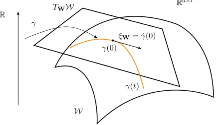
Following Absil et al. (2008), an abstract gradient descent algorithm generalizing (2.11) to Riemannian matrix manifold search spaces is given by the update formula
Wt+1 =RWt(−stgradf(Wt)). (2.12) The meaning of formula (2.12) is as follows. The Riemannian gradient gradf(Wt) is an element of the tangent space TWtW at Wt, that locally encodes the set of search directions that are consistent with the geometry of the search space. The Riemannian gradient depends on the chosen Riemannian metric gW, which is a smoothly varying inner product between elements
of the tangent space TWW at W. The scalar st > 0 is the step size. The retraction RWt is a mapping from the tangent space TWtW to the Riemannian manifold W. The retraction allows us to efficiently update the search variable Wand to maintain it within the search space of interest. Under mild conditions on the retraction RWt, the classical convergence theory of line-search algorithms in vector spaces generalizes to Riemannian manifolds (Absil et al., 2008). A conceptual illustration of the update formula (2.12) is provided in Figure 2.1. For more details, we refer the reader to Chapter 3 that explains these concepts in more details and covers the necessary material that allows us to design optimization algorithms.
2.4 Linear regression in vector search spaces
We first consider the case where the parameter of the linear regression model is ad-dimensional vectorw. The data input spaceX isRd and the considered regression model writes as
ˆ
W TWW
Wt
Wt+1
−gradf(Wt)
Figure 2.1: Conceptual illustration of a gradient descent step on a Riemannian manifoldW. The search direction gradf(Wt) belongs to the tangent space TWtW at point Wt. The retraction mapping automatically maintains the updated point Wt+1 inside the manifold.
2.4.1 Linear regression in Rd
The simplest example of linear regression problem in vector spaces is obtained when the search space W is Rd. Linear regression in Rd is a fundamental problem, central to many science
disciplines: biology, social and behavioral sciences, finance and economics, just to name a few. It was originally discussed by Legendre (1805) and Gauss (1809) who were both interested in determining comet orbits from astronomical observations. The statistical foundations of the method date back from the early 1900’s and were pioneered by Yule (1897) and Pearson et al. (1903). The corresponding least square optimization problem is typically formulated as
min
w∈RdEx,y{f(w)}, with f(w) = 1 2(w
Tx−y)2, (2.14)
and an online gradient descent algorithm for solving (2.14) is then given by,
wt+1=wt−st(wTtxt−yt)xt. (2.15)
This algorithm is both known as the Widrow-Hoff algorithm or the Least Mean Square (LMS) algorithm. As an aside, observe that (2.15) can be interpreted as a particular case of (2.12). The Euclidean metric turns Rd into a (flat) Riemannian manifold. For a scalar function f :Rd→R
of w, and the usual metricgw(δ1,δ2) =δT1δ2, the gradient satisfies
Df(w)[δ] =δTgradf(w),
where Df(w)[δ] is the directional derivative off in the direction δ,
Df(w)[δ] = lim
t→0
f(w+tδ)−f(w)
t .
In the case of interest, the gradient of the cost function is given by
gradf(w) = (ˆyt−yt)xt= (wTtxt−yt)xt, (2.16)
and the natural retraction
wt+1=Rwt(−st gradf(wt)) =wt−st gradf(wt), (2.17)
induces a line-search along “straight lines”, which are paths of shortest length in Euclidean spaces. Combining the gradient (2.16) with the retraction (2.17), one arrives at (2.15).
2.4.2 Linear regression with positive weights
A variant of the previous regression problem is obtained when the parameter is restricted to be a vector with positive entries, that is,wi >0,i= 1, ..., d. The search space is then W =Rd+.
To handle this variant of the problem, Kivinen and Warmuth (1997) propose the exponen-tiated gradient descent algorithm
wt+1=wtexp(−st(wTtxt−yt)xt), (2.18)
wheredenotes element-wise multiplication. Vector exponential is also performed element-wise. Obviously, this iteration preserves positive entries,wt>0⇒wt+1>0. The variant wherewis a probability vector, that is, wi >0 and Pdi=1wi = 1, can also be handled by normalizing the
parameter wat each iteration so that the components add up to one.
The exponentiated gradient algorithm is well-known in the context of boosting algorithms, where it appeared in the first version of the AdaBoost algorithm (Freund and Schapire, 1997). Boosting and exponentiated gradient also have a nice geometric interpretation in terms of en-tropy based projections (see Kivinen and Warmuth, 1999).
The exponentiated gradient update (2.18) can be interpreted as a particular case of (2.12). Indeed, the log-Euclidean representation
w= exp(s), s∈Rd,
where exponentiation is performed element wise, is a global diffeomorphism from Rd to Rd+. With the usual Euclidean metric gw(δ1,δ2) = δT1δ2, the gradient of the considered quadratic cost function is again given by (2.16), and the retraction
Rwt(−st gradf(wt)) =wtexp(−st gradf(wt)), (2.19)
induces a line-search in Rd+. Combining (2.16) with (2.19), one recovers update (2.18).
2.5 Linear regression in matrix search spaces
We now turn to the case where the parameter of the linear regression model is a matrix.
2.5.1 Linear regression on orthogonal matrices
Given data x ∈ Rd, observations y ∈
Rd, and a regression model ˆy = Qx the purpose is to
compute an orthogonal matrixQ that solves the optimization problem
min Q∈O(d)Ex,y{f(Q)}, withf(Q) = 1 2kQx−yk 2 2,
where O(d) is the orthogonal group, that is, the set ofd-by-dorthogonal matrices
O(d) ={Q∈Rd×d:QQT =QTQ=I}.
The learning of an orthogonal matrix has applications in various fields (see Arora, 2009, and ref-erences therein). As a linear transformation, an orthogonal matrix acts as a rotation. Therefore, the set O(d) is often referred to as the set of rotation matrices.
In the batch setting, that is, when all the samples (x1,y1), ...(xn,yn) are available up front, the problem is known as the orthogonal Procrustes problem (Schonemann, 1966),
min
Q∈O(d)||QX−Yk 2

![Figure 3.2: Quotient manifolds are defined such that equivalent points X ∼ W in the total space W correspond to a single point [W] = π(W) on the quotient space W/ ∼.](https://thumb-us.123doks.com/thumbv2/123dok_us/787235.2599531/38.892.279.596.245.503/figure-quotient-manifolds-defined-equivalent-points-correspond-quotient.webp)