University of Pennsylvania
ScholarlyCommons
Finance Papers
Wharton Faculty Research
2006
A Consumption-Based Model of the Term
Structure of Interest Rates
Jessica A. Wachter
University of PennsylvaniaFollow this and additional works at:
http://repository.upenn.edu/fnce_papers
Part of the
Finance Commons, and the
Finance and Financial Management Commons
This paper is posted at ScholarlyCommons.http://repository.upenn.edu/fnce_papers/378
For more information, please [email protected].
Recommended Citation
Wachter, J. A. (2006). A Consumption-Based Model of the Term Structure of Interest Rates.Journal of Financial Economics, 79(2), 365-399.http://dx.doi.org/10.1016/j.jfineco.2005.02.004
A Consumption-Based Model of the Term Structure of Interest Rates
AbstractThis paper proposes a consumption-based model that accounts for many features of the nominal term structure of interest rates. The driving force behind the model is a time-varying price of risk generated by external habit. Nominal bonds depend on past consumption growth through habit and on expected inflation. When calibrated to data on consumption, inflation, and the aggregate market, the model produces realistic means and volatilities of bond yields and accounts for the expectations puzzle. The model also captures the high equity premium and excess stock market volatility.
Disciplines
The Rodney L. White Center for Financial Research
A Consumption-Based Model of the
Term Structure of Interest Rates
Jessica A. Wachter 27-04
A Consumption-Based Model of the Term Structure
of Interest Rates
∗Jessica A. Wachter†
University of Pennsylvania and NBER
July 9, 2004
∗I thank Andrew Ang, Ravi Bansal, Michael Brandt, Geert Bekaert, John Campbell, John Cochrane,
Francisco Gomes, Vassil Konstantinov, Martin Lettau, Anthony Lynch, David Marshall, Lasse Pederson, Andre Perold, Ken Singleton, Christopher Telmer, Jeremy Stein, Matt Richardson, Stephen Ross, Robert Whitelaw, Yihong Xia, seminar participants at the 2004 Western Finance Association meeting in Vancouver, the 2003 Society of Economic Dynamics meeting in Paris, and the 2001 NBER Asset Pricing meeting in Los Angeles, the the NYU Macro lunch, the New York Federal Reserve, Washington University, and the Wharton School. I thank Lehman Brothers for financial support.
†Address: The Wharton School, University of Pennsylvania, 3620 Locust Walk, Philadelphia, PA 19104;
A Consumption-Based Model of the Term Structure
of Interest Rates
Abstract
This paper proposes a consumption-based model that can account for many features of the nominal term structure of interest rates. The driving force behind the model is a time-varying price of risk generated by external habit. Nominal bonds depend on past consumption growth through habit and on expected inflation. When calibrated to data on consumption, inflation, and the average level of bond yields, the model produces realistic volatility of bond yields and can explain key aspects of the expectations puzzle documented by Campbell and Shiller (1991) and Fama and Bliss (1987). When actual consumption and inflation data are fed into the model, the model is shown to account for many of the short and long-run fluctuations in the short-term interest rate and the yield spread. At the same time, the model captures the high equity premium and excess stock market volatility.
Introduction
The expectations puzzle, documented by Campbell and Shiller (1991) and Fama and Bliss (1987), has long posed a challenge for general equilibrium models of the term structure. Backus, Gregory, and Zin (1989) show that a model assuming power utility preferences and time-varying expected consumption growth cannot account for this puzzle. Although Dai and Singleton (2002) show that a statistical model of the stochastic discount factor can fit the puzzle, this only raises the question of what economic mechanism is at work.
This paper proposes a consumption-based model that captures key aspects of the empirical results of Campbell and Shiller (1991) and Fama and Bliss (1987). Campbell and Shiller run the regression y$n,t+1−y$nt= constant +βn 1 n−1(y $ nt−y$1t) + error,
where y$nt =−n1lnPnt$, andPnt$ is the price of a nominal bond with maturityn. According to the expectations hypothesis, excess returns on bonds are unpredictable, and all the variation in yield spreads is due to variation in future short-term interest rates. In terms of the regression above, this meansβn= 1 for all n. But Campbell and Shiller show, on the contrary, that βn is less than one
and decreasing in n. The model in this paper reproduces these findings. The model also generates an upward sloping average yield curve (as found in the data) and realistic bond yield volatility.
Two ingredients enable the model to capture these findings. The first is external habit persis-tence from Campbell and Cochrane (1999). Habit persispersis-tence generates time variation in investor preferences. After periods of unusually low consumption growth, the volatility of investors’ marginal utility rises, causing them to demand greater premia on risky assets. As a result, the risk premium on the aggregate stock market varies in a countercyclical fashion.
Habit utility preferences are clearly not enough: In the model of Campbell and Cochrane (1999), the riskfree rate is constant and the term structure is trivial. The second ingredient is thus a model for the short-term interest rate that makes long-term bonds risky in the first place. Without this ingredient, it is impossible for long-term bonds to have positive, countercyclical risk premia.
In this paper, the short-term real interest rate varies with surplus consumption, the ratio be-tween current consumption minus a slow-moving weighted average of past consumption, and current consumption. The estimated model implies that surplus consumption and the real riskfree rate are negatively correlated; when past consumption growth is relatively low, investors borrow to give habit a chance to catch up to consumption. However, an increase in precautionary savings
miti-gates the effect, keeping the volatility of the interest rate low. The negative correlation between surplus consumption and the riskfree rate leads to positive risk premia on real bonds, and an upward sloping yield curve.
In order to speak to the empirical findings in the term structure, it is necessary to model nominal as well as real bonds. This paper assumes an exogenous affine process for the price level. The affine assumption allows for a tractable solution to the nominal bond pricing problem. Nominal bonds are influenced by expected inflation as well as by surplus consumption growth. Expected inflation is calibrated purely to match inflation data. Thus the factors driving interest rates and bond returns in this model are based in macroeconomics, rather than on asset prices.1
Besides the empirical literature on the expectations hypothesis, this paper draws on the earlier literature on habit formation (e.g., Abel (1990), Chapman (1998), Constantinides (1990), Dybvig (1995), Ferson and Constantinides (1991), Heaton (1995), and Sundaresan (1989)). Constantinides (1990) and Sundaresan (1989) show that habit formation models can be used to explain a high equity premium with low values of risk aversion. Like these models, the model proposed here assumes that the agent evaluates today’s consumption relative to a reference point that increases with past consumption. Following Campbell and Cochrane (1999), this paper departs from earlier work by assuming that habit is external to the agent, namely that the agent does not take into account future habit when deciding on today’s consumption. Abel (1990) also assumes external habit formation, but in his specification, agents care about the ratio of consumption to habit, rather than the difference. As a result, risk aversion is constant and risk premia do not vary through time. 2 Motivated by habit formation models, Li (2001) examines the ability of past consumption growth to predict excess returns on stocks. However, Li does not look at the predictive ability of consumption for short or long-term interest rates, nor does he consider the implications for habit formation for the expectations hypothesis.
An intriguing feature of the model in this paper is the link it produces between asset returns and
1Ang and Piazzesi (2003) also investigate the role of macroeconomic variables in the term structure. They consider
an affine term structure model where output and inflation are among the factors. Evans and Marshall (2003) consider the extent to which macroeconomic shocks can explain changes in yields, where the macroeconomic shocks are inferred using restrictions from general equilibrium models.
2Lately there has been increased interest in the empirical properties of habit formation models. Dai (2000)
links the Constantinides model to a model for labor income. Brandt and Wang (2003) study habit preferences over inflation. Bekaert, Engstrom, and Grenadier (2004) consider a model where the investor’s reference point is imperfectly correlated with past consumption. Menzly, Santos, and Veronesi (2004) introduce a variant of the Campbell and Cochrane model to explain returns on industry portfolios. Chen and Ludvigson (2003) evaluate habit specifications using nonparametric methods.
underlying macroeconomic variables. When actual consumption and inflation data is fed through the model, the implied nominal riskfree rate has a correlation of .72 with the 3-month Treasury yield in the data. The implied spread between the five-year and three-month yield has a correlation of .40 with the yield spread in the data. This is in spite of the fact that the returns implied by the model are driven only by consumption growth and inflation. When expectations-hypothesis regressions are adjusted by implied risk premia on bonds, as proposed by Dai and Singleton (2002), the violation of the expectations hypothesis is reduced by more than half at the long end of the term structure. Finally, the model preserves the advantages of the original Campbell and Cochrane (1999) framework. It successfully captures the high equity premium for the aggregate market, excess volatility, and predictability of excess stock returns.
The outline of the paper is as follows. Section 1 describes the assumptions on the endowment, preferences, and the price level, and how the model is solved. Section 2 describes the estimation of the inflation process. Section 3 describes the calibration and the implications for the population moments of asset returns, and for the time series of asset returns in the postwar data.
1
Model
This section describes the model assumed in this paper. Section 1.1 describes the assumptions for preferences, Section 1.2 describes the assumptions on the price level. Section 1.3 describes the solution method, and Section 1.4 discusses consequences for risk premia on real and nominal bonds.
1.1 Preferences
Assume that an investor has utility over consumption relative to a reference point Xt:
E ∞ X t=0 δt(Ct−Xt) 1−γ−1 1−γ . (1)
Habit,Xt, is defined indirectly, through surplus consumption St, where
St≡
Ct−Xt
Ct
.
To ensure thatXt never falls belowCt,st= lnSt is modeled:
st+1= (1−φ)¯s+φst+λ(st)(∆ct+1−E(∆ct+1)), (2) The process for st is heteroscedastic, and perfectly correlated with innovations in consumption
The investor’s habit is external: the investor does not take into account the effect that to-day’s consumption decisions have on Xt in the future.3 Because habit is external, the investor’s
intertemporal marginal rate of substitution is given by:
Mt+1=δ µ St+1 St Ct+1 Ct ¶−γ . (3)
Following Campbell and Cochrane (1999), consumption is parametrized as a random walk:
∆ct+1 =g+vt+1 (4)
wherevt+1is aN(0,1) shock that is independent across time. As shown in Campbell and Cochrane (1999), this specification implies thatxt is approximately a weighted average of past consumption
growth, as would be expected from an external habit formation model. From the Euler equation, it follows that the real riskfree rate equals
rf,t+1 = ln (1/Et[Mt+1])
= −lnδ+γg+γ(1−φ)(¯s−st)−
γ2σ2v
2 (1 +λ(st))
2. (5) This riskfree rate has some familiar terms from the power utility case and others that are new to habit formation. As in the power utility model, positive expected consumption growth leads investors to borrow from the future to smooth consumption. This is reflected in the term γg
(however,γis not equal to risk aversion as it is under power utility). The second term, proportional to ¯s−st, implies that as surplus consumption falls relative to its long-term mean, investors borrow
more. This is due to the mean-reverting nature of surplus consumption: investors borrow against future periods when habit has had time to adjust and surplus consumption is higher. The last term reflects precautionary savings. A higher λ(st) implies that surplus consumption, and therefore
marginal utility, is more volatile. Investors increase saving, and rf falls.
The function λ(st) is chosen so that the intertemporal substitution and precautionary savings
effects offset each other, and so that the model has intuitive properties of habit formation. Campbell and Cochrane choose the function so that these effects are completely offset and the riskfree rate is constant. In contrast, this paper allows the data to determine the net effect of ston the riskfree
rate. For simplicity,λ(st) is restricted so that rf,t+1 is linear in st. In addition,λ(st) is chosen so
3Formally,X
tcan be considered as aggregate habit and the agent as evaluating consumption relative to aggregate habit. Because all agents are identical, individual consumption and habit and aggregate consumption and habit can be treated interchangeably.
that forst≈¯s,xtis a deterministic function of past consumption. These considerations imply that λ(st) = (1/S¯) p 1−2(st−s¯)−1 (6) ¯ S = σv r γ 1−φ−b/γ. (7)
In order that the quantity within the square root remain positive,λ(st) is set to be 0 whenst> smax, for smax= ¯s+ 1 2 ¡ 1−S¯2¢ . (8)
st ventures above smax sufficiently rarely that this feature does not affect the behavior of the model. More details can be found in Appendix A.1. Substituting these equations into (5) reduces the riskfree rate equation to
rf,t+1 = µ −lnδ+γg− γ(1−φ)−b 2 ¶ +b(¯s−st) (9)
where b is a free preference parameter that will be estimated from the data, and ¯rf equals the
unconditional mean of rf,t+1.
Equations (5) and (9) indicate that the parameter bhas an economic interpretation. If b >0, the intertemporal smoothing effect wins out, and an increase in surplus consumption st drives
down the interest rate. If b <0, the precautionary savings effect wins out. An increase in surplus consumptionstdecreases the sensitivityλ(st) and drives up the interest rate. Settingb= 0 results
in a constant real interest rate, and gives the model of Campbell and Cochrane (1999).4
While the functional form of λ(st) is chosen to match the behavior of the riskfree rate, it has
important implication for returns on risky assets. It follows from the investor’s Euler equation that
Et(Rt+1−Rf,t+1) σt(Rt+1) =−ρt(Mt+1, Rt+1) σt(Mt+1) Et(Mt+1) ,
whereRt+1 is the return on some risky asset. As a consequence
Et(Rt+1−Rf,t+1)
σt(Rt+1) ≈ −
ρt(Mt+1, Rt+1)γσv2(1 +λ(st)), (10)
which follows from the lognormality of Mt+1 conditional on time-t information. Because λ(st)
is decreasing in st, the ratio of the volatility of the stochastic discount factor to its mean varies
4Campbell and Cochrane briefly consider the case ofb6= 0 in the working paper version of their model, Campbell
and Cochrane (1995), but examine only the real term structure, and do not discuss implications for nominal bonds, long rate regressions, or for the time series of interest rates and risk premia. These are the focus of this paper.
countercyclically. This provides a mechanism by which Sharpe ratios, and hence risk premia, vary countercyclically over time.5
In the model of Campbell and Cochrane (1999), the mechanism in (10) does not create time-varying risk premia on bonds for the simple reason that bond returns are constant, and equal to the riskfree rate at all maturities. In terms of (10), the Campbell and Cochrane model implies that
ρt(Mt+1, Rt+1) = 0, whenRt+1is the return on a bond. However, the model in this paper generates a time-varying riskfree rate. Therefore ρt(Mt+1, Rt+1) is nonzero, and (10) provides a mechanism for risk premia on real bonds, as well as risk premia on stocks, to vary through time. Of course, this observation alone does not solve the expectations puzzle. The sign of bond premia, and the magnitude of time-variation will depend on the results of the parameter estimation.
1.2 Inflation
To model nominal bonds, it is necessary to introduce a process for inflation. For simplicity, we follow Boudoukh (1993) and Cox, Ingersoll, and Ross (1985), and model inflation as an exogenous process.6 Let Π
t denote the exogenous price level and πt = ln Πt. It is assumed that log inflation
follows the process:
∆πt+1=η0+ηZt+σπ²t+1. (11) Here Zt is anm×1 vector of state variables that follow a vector-autoregressive process:
Zt+1 =µ+ ΦZt+ Σ²t+1, (12) where Φ is an m×m matrix and µis an m×1 vector. The correlation between inflation, Zt and
consumption can be modeled in a parsimonious way by writing the consumption growth shockvt+1 as
vt+1=σc²t+1
Here,²t+1is an (m+2)×1 vector of independentN(0,1), random variables,σcandσπare 1×(m+2)
and Σ is m×(m+ 2).
This structure allows for an arbitrary number of state variables and cross-correlations. In addition, the state variables may be correlated with consumption growth or changes in the price level. Multiple lags may be accommodated by increasing the dimension ofZt.
5Harvey (1989) provides direct evidence that the the risk-return tradeoff varies counter-cyclically.
6Since an earlier version of this paper circulated, Buraschi and Jiltsov (2003) study a related model that puts the
money supply directly in the utility function. They focus on the dynamics of inflation and the inflation risk premium, rather than the link between the term structure and consumption, which is the focus here.
1.3 Model Solution
This section calculates the prices of long-term bonds and stocks. To compute prices on nominal bonds, techniques from affine bond pricing7 are combined with numerical methods. Introducing affine bond pricing techniques improves the efficiency of the calculation and provides insight into the workings of the model.
Bond Prices
This paper solves for prices of both real bonds (bonds whose payment is fixed in terms of units of the consumption good) and nominal bonds (bonds whose payoff is fixed in terms of units of the price level). As shown below, the assumption that expected inflation follows a multivariate auto-regressive process with Gaussian errors implies that bond yields are exponential affine in expected inflation. Following Campbell and Viceira (2001), let Pn,t denote the real price of a real bond
maturing in n periods, and Pn,t$ the nominal price of a nominal bond. The real return on an
n-period real bond is given by:
Rn,t =
Pn−1,t+1
Pn,t
withrn,t= lnRn,t. The nominal return on an n-period nominal bond is:
Rn,t$ = P $ n−1,t+1 Pn,t$ withr$n,t= lnR$n,t. Finally, yn,t=− 1 nlnPn,t and y$n,t=−1 nlnP $ n,t
denote the real yield on the real bond and the nominal yield on the nominal bond respectively. Bond prices are determined recursively by the investor’s Euler equation. For real bonds, this translates into: Pn,t=Et " δ µ St+1 St Ct+1 Ct ¶−γ Pn−1,t+1 # . (13)
7See Backus, Foresi, and Telmer (2001) and Sun (1992) for illustrations of this approach in discrete-time and Duffie
and Kan (1996) for an illustration in continuous time. Bakshi and Chen (1996), Bekaert, Engstrom, and Grenadier (2004) and Brennan, Wang, and Xia (2003) apply this approach to the pricing of bonds and equities.
When n = 0, the bond is worth one unit of the consumption good. This implies the boundary condition:
P0,t= 1.
For nominal bonds, the Euler equation implies that:8
Pn,t$ =Et " δ µ St+1 St Ct+1 Ct ¶−γ Πt Πt+1 Pn$−1,t+1 # (14) with P0$,t= 1.
Note that rf,t+1 =r1,t+1=y1,t, and rf,t$ +1=r1$,t+1=y1$,t.
Because the distribution of future consumption and surplus consumption depends only on the state variablest, (13) implies that real bond prices are functions ofst alone:
Pn,t=Fn(st) withF0(st) = 1, and Fn(st) = Et " δ µ St+1 St Ct+1 Ct ¶−γ Fn−1(st+1) # (15) = Et[exp{lnδ−γg−γ(1−φ)(¯s−st)−γ(λ(st) + 1)σc²t+1}Fn−1(st+1)] (16) Equation (16) can be solved using numerical integration on a grid of values forst. For this problem,
numerical integration is superior to calculating the expectation by Monte Carlo. This is because the sensitivity of asset prices to rare events makes simulation unreliable.
Equation (14) indicates that, unlike real bond prices, nominal bond prices are functions of the state variable Zt as well as st. This potentially complicates the solution for nominal bond
prices, because time-varying expected inflation introduces, at the least, one more state variable. Fortunately, a simply trick can be used to reduce computation time back to what it would be for
8The equations for nominal bond prices follow from the fact that the Euler equation must hold for real prices of
nominal bonds. Therefore:
Pn,t$ Πt =Et " Mt+1 P$ n−1,t+1 Πt+1 #
In real terms, the nominal bond maturing today is worth
P0$,t Πt
= 1 Πt
a single state variable. Using the law of iterated expectations and conditioning on realizations of the shockvt+1=σcεt+1, it can be shown that nominal bond prices take the form:
Pn,t$ =Fn$(st) exp{An+BnZt}. (17)
The functionsF$
n can be solved by one-dimensional numerical integration:
Fn$(st) = Et h Mt+1exp{ξnσc²t+1}Fn$−1(st+1) i = Et h exp{lnδ−γg−γ(1−φ)(¯s−st) + (ξn−γ(λ(st) + 1))σc²t+1}Fn$−1(st+1) i
while An and Bn are defined recursively by:
An = An−1−η0+Bn−1µ+ 1 2(Bn−1Σ−σπ) £ I−σ0c(σcσc0)−1σc ¤ (Bn−1Σ−σπ)0 (18) Bn = Bn−1Φ−η (19) and ξn= (Bn−1Σ−σπ)σc0(σcσ0c)−1. (20)
The boundary conditions are F0$(st) = 1, A0 = 0,B0 = 01×m. The last term in (18) follows from
Jensen’s inequality: because inflation is log-normally distributed, the volatility of inflation works to decrease bond yields at long maturities. These formulas can also be used to gain insight into the workings of the model, as explained in Section 1.4.
Aggregate Wealth
In this economy, the market portfolio is equivalent to aggregate wealth, and the dividend equals aggregate consumption. The price-consumption ratio and the return on the market can be calcu-lated using methods similar to those above, with a small but important modification. Analogously to the previous section, let Pe
n,t denote the price of an asset that pays the endowment Ct+n in n
periods. The e superscript denotes equity. Because these assets pay no coupons, they have the same recursive pricing relation as bonds (16). Of course the prices are different, and this is because there is a different boundary condition:
P0e,t =Ct.
Unlike the case for bonds, Pe
n,t is not simply a function of st. It is a function of consumption Ct
as well. To avoid introducing an additional variable into the problem, the equations for equity are rewritten in terms of price-consumption ratios, rather than simply prices.
Pe n,t Ct =Et " δ µ St+1 St ¶−γµ Ct+1 Ct ¶1−γPe n−1,t+1 Ct+1 # . (21)
with boundary condition P
e
0,t
Ct = 1. Now the problem is analogous to that for bond pricing. The
ratio of the price zero-coupon equity to aggregate consumption can be written as a functionFe n of
st, where
Fne(st) =Et £
exp{lnδ+ (1−γ)g−γ(1−φ)(¯s−st) + (1−γ(λ(st) + 1))σc²t+1}Fne−1(st+1)¤ with boundary conditionFe
n(st) = 1. This formula can be solved recursively using one-dimensional
quadrature.
Finally, the price-consumption ratio of the market equals the sum of the price-consumption ratio on these zero-coupon securities:
Pt Ct = ∞ X n=1 Pn,te Ct . (22)
This way of calculating the price-consumption ratio is equivalent to the more traditional fixed-point method used by Campbell and Cochrane (1999). In this endowment economy, (22) also represents the price-dividend ratio.
1.4 Implications for bond risk premia
The nominal return on the one-period nominal bond (the nominal riskfree rate) can be determined using these equations, or directly from (14):
rf,t$ +1 = −lnδ+γg−γ(1−φ)−b 2 +b(¯s−st) + (η0+ηZt)−σπσ 0 cγ(λ(st) + 1)− 1 2σπσ 0 π = rf,t+1+Et[∆πt+1]−1 2σπσ 0 π−σπσ0cγ(λ(st) + 1) (23)
Of interest is the risk premium on the nominal riskfree asset. Subtracting the real riskfree rate from the expected real return on the one-period nominal bond produces:
Et[rf,t$ +1−∆πt+1]−rf,t+1 =−σπσc0γ(λ(st) + 1)−
1 2σπσ
0
π
The term 12σπσ0π is an adjustment for Jensen’s inequality. If σπσc < 0, the one-period nominal
bond has a positive risk premium relative to the one-period real bond. Intuitively, this is because
σπσc0 <0 implies that inflation and consumption growth are negatively correlated. Because higher
inflation lowers the return on the nominal riskfree bond, a negative correlation between inflation and consumption implies that the nominal bond pays off when investors need the money least. Therefore the one-period nominal bond carries a risk premium relative to the one-period real bond.
The formulas derived in Section 1.3 can be used to show that nominal risk premia depend only on St. It follows from (17) that
Et[rn,t$ +1] = Et h lnFn$−1(st+1)−lnFn$(st) +An−1−An+Bn−1Zt+1−BnZt i = constant +Et[lnFn$−1(st+1)]−lnFn$(st) + (Bn−1Φ +Bn)Zt = constant +Et[lnFn$−1(st+1)]−lnFn$(st) +ηZt Moreover, r1$,t+1= constant +b(¯s−st) +ηZt−σπσc0γ(λ(st) + 1)
(recall thatr$1,t+1 =r$f,t+1). Therefore nominal risk premia depend only on st:
Et[rn,t$ +1−r1$,t+1] = constant +Et[lnFn$−1(st+1)]−lnFn$(st)−b(¯s−st) +σπσc0γ(λ(st) + 1) (24)
In general, there is no closed form expression for nominal or real bond prices with maturity greater than one period. These can be determined in some special cases, as described below.
Special cases
Suppose first thatb= 0. Then the real riskfree rate is constant:
rf,t+1=rf.
Moreover, it follows from (14) that
Pn,t= exp{−nrf}. (25)
(25) can be shown using induction. IfPn−1,t = exp{−(n−1)rf}, then
Pn,t=Et[Mt+1exp{−(n−1)rf}] =Et[Mt+1] exp{−(n−1)rf}= exp{−nrf}.
Moreover, risk premia are zero in this case.
Nominal bonds are a different story. As long as expected inflation varies, the nominal riskfree rate also varies. Even if b= 0, correlation between expected and unexpected inflation creates risk premia on nominal bonds. These risk premia vary with st, and it is again not possible to solve for
bond prices in closed form. Suppose however that Σσ0
c = 0 and σπσ0c = 0. Then inflation risk is
not priced, and the same reasoning as above shows that
Substituting in from (12), (18), and (19), it follows that Et[r$n,t+1] = rf +η0+ηZt− 1 2(Bn−1−σπ)(Bn−1Σ−σπ) 0 = rf,t$ +1+1 2σπσ 0 π− 1 2(Bn−1−σπ)(Bn−1Σ−σπ) 0
Thus risk premia on nominal bonds are zero except for a constant Jensen’s inequality term.
2
Estimation
The results of the previous section suggest that the process assumed for expected inflation will be an important determinant of yields and returns on nominal bonds. This section focuses on estimating this process.
A special case of the model presented in Section 1.2 is considered. I assume that expected inflation follows an AR(1) process, namely that Zt is univariate. This is equivalent to assuming
that realized inflation follows an ARMA(1,1) process. The advantage of this approach is that estimation via maximum likelihood is straightforward, and, as shown below, the resulting expected inflation series appears to capture much of the variation in realized inflation.
Model calibration requires not only the parameters of the inflation process, but also mean consumption growth, the variance of consumption growth, and the correlation between consumption and inflation. For simplicity, aggregate consumption growth is assumed to be independent and identically distributed across time. However, the literature has identified a number of reasons
why measured consumption may exhibit temporal dependence (e.g. Christiano, Eichenbaum, and
Marshall (1991), Ferson and Harvey (1992), Heaton (1993)). To account for this dependence in the estimation, we assume that inflation and consumption growth each follow an ARMA(1,1) with correlated errors. That is, I estimate
∆ct+1 = (1−ψ1)g+ψ1∆ct+θ1ν1,t+ν1,t+1 (26) ∆πt+1 = (1−ψ2)¯π+ψ2∆πt+θ2ν2,t+ν2,t+1 (27) where " ν1,t+1 ν2,t+1 # ∼N Ã 0, " σ12 σ1σ2ρ σ1σ2ρ σ22 #! (28)
Here, ψ1 is the auto-regressive coefficient for mean consumption growth, while, θ1 is the moving-average coefficient. Similarly,ψ2 is the auto-regressive coefficient of inflation, while θ2 is inflation’s moving-average coefficient. The parameter ρ represents the correlation between innovations to
consumption growth and innovations to inflation. Equations (26)–(28) imply an exact likelihood function, derived in Appendix A.3. Section 3.1 describes the mapping from the parameters assumed in this section to the parameters assumed in Section 1.2.
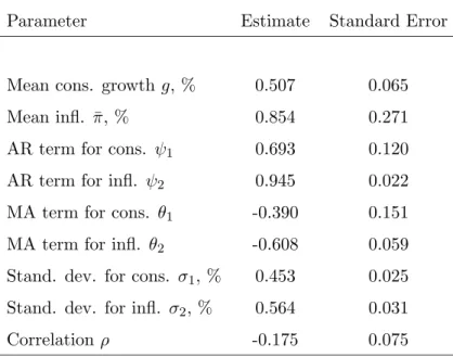
Equations (26)–(28) are estimated via maximum likelihood using quarterly data on inflation and consumption from 1952 to 1998. Per-capita data on consumption of non-durables and services comes from the Board of Governors of the Federal Reserve, and is available from Martin Lettau’s website. This data is inflation-adjusted. See Lettau and Ludvingson (2001) for a further description of this data. Quarterly data on the consumer price index is taken from CRSP. Table 1 shows the results of the estimation: The left column reports the parameter estimate, the right column reports the standard error. All parameters are in quarterly units, and means and standard deviations are in percentages. Mean quarterly consumption growth (g) over this period is 0.51%, while mean inflation (¯π) is 0.85%. The estimates indicate that expected inflation is highly persistent, with an auto-regressive coefficient of 0.94. The correlation between innovations to consumption and innovations to inflation is -0.18.
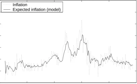
Figure 1 plots the time series of quarterly realized inflation together with the time series of expected inflation implied by (26)-(28) and the estimates in Table 1. As described in Appendix A.3, this series is constructed recursively using past inflation data. Figure 1 shows that the expected inflation series captures many of the lower-frequency fluctuations in realized inflation. Indeed, the expected inflation series implied by this process explains 54% of the variance of realized inflation.
The next section combines the estimation results of this section with the formulas of Section 1 to determine the implications of the model for the nominal term structure.
3
Implications for Asset Returns
This section describes the implications of the model for returns on bonds and stocks. Section 3.1 describes the calibration of the parameters, and the data used to calculate moments of nominal bonds for comparison. Section 3.2 characterizes the price-dividend ratio and the yield spread on real and nominal bonds as functions of the underlying state variables st and expected inflation.
Section 3.3 evaluates the model by simulating 100,000 quarters of returns on stocks and nominal and real bonds and compares the simulated moments implied by the model to those on stocks and nominal bonds in the data. Lastly, Section 3.4 shows the implications of the model for the time series of the short-term interest rate and the yield spread, and examines the properties of implied bond risk premia using the technique proposed by Dai and Singleton (2002).
3.1 Calibration
The processes for consumption and inflation are calibrated using the estimation of Section 2, while the preference parameters are calibrated using bond and stock returns.9 Clearly the parameteriza-tion in Secparameteriza-tion 1.2 is under-identified, so certain parameters must be fixed. First, note that
" σc σπ # [σc0 σ0π] = " σ21 σ1σ2ρ σ1σ2ρ σ22 # (29)
In order to identifyσc andσπ, assume that the matrix "
σc
σπ #
is lower triangular. Thenσc andσπ
can be found by taking the Cholesky decomposition of the right hand side of (29).
Assume µ= 0 and η= 1. Then the remaining parameters can be identified as follows.
η0 = ¯π (30)
Φ = ψ2 (31)
Σ = (ψ2+θ2)σΠ. (32) The resulting process for inflation is identical to (27). This follows from solving for Zt in (11) and
substituting the resulting expression into (12). Under assumptions (30) – (32) (with µ = 0 and
η1 = 1), it follows that
∆πt+1−π¯−σπεt+1=ψ(∆πt−π¯−σπεt) + (ψ2+θ2)σπεt.
Solving for ∆πt+1 and applying (29) produces (27).
Note that under this specification, expected inflation and realized inflation are assumed to be perfectly positively correlated. This assumption allows expected inflation to be identified from inflation data alone. As explained in Section 2, the ARMA parameters for consumption growth are set equal to zero. This is in part for simplicity and in part because these parameters capture pre-dictability due to data construction, rather than prepre-dictability in underlying consumption growth itself.
Once consumption and inflation are determined, there remain four parameters of the investor’s utility function that need to be identified. These are the discount rateδ, the utility curvature,γ, the
9This calibration strategy is similar to that used in Boudoukh (1993), who investigates a term structure model
where investors have power utility and consumption and inflation follow a vector-autoregression with heteroscedastic errors. Boudoukh fits consumption and inflation parameters to consumption and inflation data, and preference parameters to bond returns.
persistence of habit,φ, and the loading of the interest rate on the negative of surplus consumption,
b. The latter parameter can be given an interpretation in terms of the utility function, as it determines the trade-off between the precautionary savings and intertemporal smoothing effects of
ston the riskfree rate.
From (9) and (23), it follows that the parameterδhas a one-to-one correspondence with the level of the riskfree rate. For this reason,δ is set so that, in population, the mean of the nominal riskfree rate matches (approximately) that in the data. Given the other parameters, and an estimate of the mean of the nominal riskfree rate in the data ¯r$, this is accomplished by setting
δ = exp ½ −r¯$+γg−γ(1−φ)−b 2 + ¯π−σπσ 0 cγ(λ(¯s) + 1)− 1 2σπσ 0 π ¾
This implies that when the nominal riskfree rate in the model is evaluated at ¯s, it equals the yield on the three-month bond. Becauseλ(st) is a non-linear function ofst, the mean in population will
not exactly equal that from the data. However, the simulation results in Section 3.3 show that the difference is small.
Because the purpose of this paper is to determine the implications for bond returns of a model that is intended to capture features of equity returns, these parameters are determined, as far as possible, by equity return data. This is possible forγ and φ, butbhas very little impact on equity returns. Therefore, we setbso that mean yield on the nominal five-year bond in the model is equal to its mean from the data. In order to generate an upward sloping yield curve, it is necessary that
b > 0, i.e. that the riskfree rate loads negatively on b (and that the intertemporal substitution effect dominates the substitution effect). If b > 0, the real riskfree rate is negatively correlated with surplus consumption. This implies bond returns will be positively correlated with surplus consumption, and thus that bond returns, both real and nominal, will have positive risk premia. Note also that the correlation between inflation and consumption is estimated to be negative. This implies that the risk premium due to inflation is positive, and further increases the premium on nominal bonds. For the numbers estimated here, however, this effect is small.
Simulation results show that the parameter φdetermines the first-order autocorrelation of the price-dividend ratio. This also is reasonable given thatP/D is a function of st alone. Thereforeφ
is set to equal 0.95, the first-order autocorrelation of the price-dividend ratio in the data. Finally,
γ is set so that the unconditional Sharpe ratio of equity returns is equal to the Sharpe ratio in the data. The parameter value choices are summarized in Table 2.
Relative to Campbell and Cochrane (1999), the free parameter in this model isb, the loading of the interest rate on the negative of surplus consumption (the inflation parameters are determined
solely from CPI data). This parameter is fit to the average yield spread between the five-year and the three-month nominal bond. However, b has time-series implications as well as cross-sectional ones. A value of b > 0 implies that surplus consumption influences the real riskfree rate with a negative sign. As a brief investigation of these time series implications, the ex-post real interest rate is regressed on a surplus consumption proxy, P40
j=1φj∆ct−j, which is approximately equal to
st. While st is, in theory, influenced by surplus consumption going back to infinity, in practice, it
is necessary to make a choice as to where to cut off past consumption. To capture the nature ofst
as a long-run variable, ten years is chosen as the cut-off point. The regression is therefore
r$f,t+1−∆πt+1 =a0+a1 40
X
j=1
φj∆ct−j+εt+1
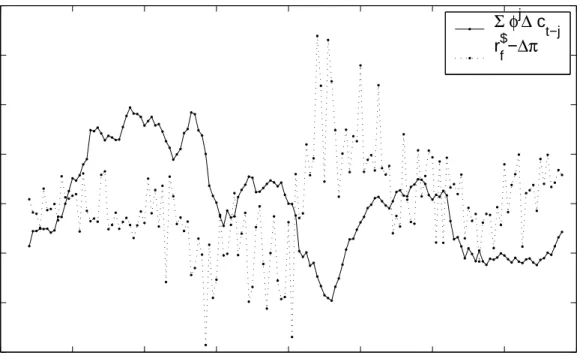
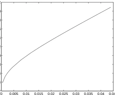
The results of this regression lend support for the choice of b > 0. The parameter a1 is found to be negative and statistically significant, with a point estimate of -0.13, and a standard error, adjusted for serial correlation and heteroskedasticity, of 0.04.10 Figure 2 plots the history of average past consumption (P40
j=1φj∆ct−j) and r$f,t+1 −∆πt+1. The negative relationship between past consumption and the ex-post real riskfree rate is apparent throughout the sample period.
Calibrating the parameters as described above, and comparing returns in the model to those in the data, requires data on nominal bond yields and on equity returns. The bond data consist of monthly observations on annual zero coupon yields for three-month, six-month, one, two, five, and ten year U.S. government bonds for the years 1952 to 1998. The data, constructed using the interpolation techniques of McCulloch and Kwon (1993) and Bliss (1997), are available from the website of Gregory Duffee. Following Campbell and Viceira (2001), I use only quarterly observations to eliminate the high-frequency fluctuations that would seem difficult to explain based on a model with macro-based variables. Monthly observations on returns on a value-weighted index of stocks traded on the NYSE and AMEX are taken from CRSP. These are used to compute quarterly returns and quarterly observations on the ratio of price to annual dividends.
3.2 Characterizing the Solution
As shown in Figure 3, the price-dividend ratio increases with surplus consumptionSt. As the
price-dividend ratio is often taken to be a measure of the business cycle (e.g. Lettau and Ludvingson (2001)), this confirms the intuition that St is a procyclical variable.
10A potential concern with this regression is the relatively high degree of persistence in the surplus consumption
ratio. A Monte Carlo exercise designed to correct for this persistence yields a 5% critical value (based on a two-tailed test) of -0.092, implying that the value of -0.13 remains significant.
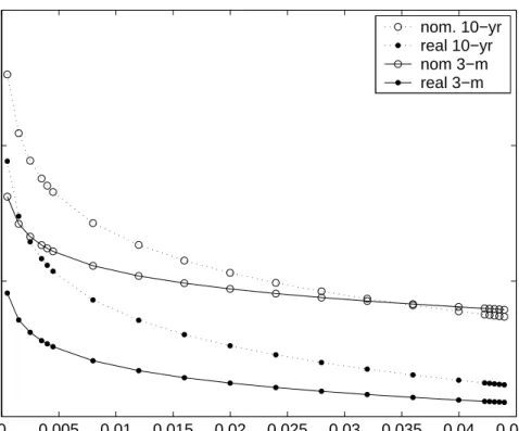
Figure 4 plots the yields on nominal and real bonds for maturities of three months and ten years. Expected inflation is set equal to its long-run mean. Both nominal and real yields decrease withSt, but the long yields are more sensitive toStthan the short yields. Thus the spread between
the long and short yields is decreasing inStfor both nominal and real yields. Figure 4 also shows
that the long-term yields generally lie above the short-term yields, and that nominal yields lie above real yields. The first of these effects follow from the fact that b >0, i.e. that the interest rate loads negatively on St, while the second effect follows primarily from the fact that expected
inflation growth is positive. For values ofStthat are very high, the ten-year yield lies slightly below
the 3-month yield. This arises because the risk premium is very low for these values of St, and is
dominated by the Jensen’s inequality term in (18)).
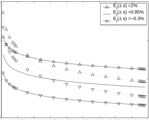
Figure 5 plots the yields on nominal bonds as functions of surplus consumptionStand expected
inflation. Expected inflation is set equal to its long-run mean of 0.85%, and varied by plus and minus two unconditional standard deviations (about 1.15%). Both long and short-term yields are increasing in expected inflation. However, the effect of expected inflation on short-term yields is greater than on long-term yields. This plot shows that two factors drive yields in the model. Expected inflation is more important at the short end of the yield curve, while surplus consumption dominates at the long end of the yield curve.
3.3 Simulation
To evaluate the predictions of the model for asset returns, 100,000 quarters of data are simulated. Prices of the claim on aggregate consumption (equity), of real, and nominal bonds are calculated numerically, using the method described in Section 1.3.
Returns on the Aggregate Market
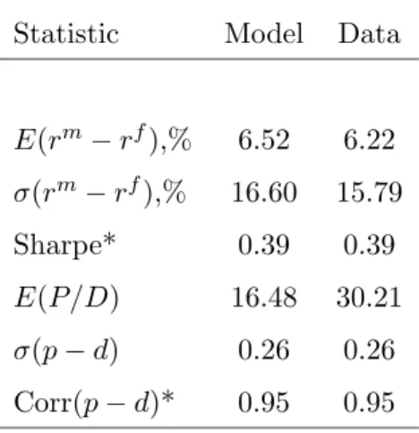
Table 3 shows the implications of this model for equity returns. Despite the difference in the parameterb, the implications of the present model for equity returns are nearly identical to those of Campbell and Cochrane (1999). The model fits the mean and standard deviation of equity returns, even though it was calibrated only to match the ratio. Thus the model can fit the equity premium puzzle of Mehra and Prescott (1985). The persistence φis chosen so that the model fits the correlation of the price-dividend ratio by construction. However, the model can also reproduce the high volatility of the price-dividend ratio, demonstrating that the model fits the volatility puzzle described by Shiller (1981). Stock returns and price-dividend ratios are highly volatile even though
the dividend process is calibrated to the extremely smooth postwar consumption data. In addition, results available from the author show that price-dividend ratios have the ability to predict excess returns on equities, just as in the data (Campbell and Shiller (1988), Fama and French (1989)), and that declines in the price-dividend ratio predict higher volatility (Black (1976), Schwert (1989), Nelson (1991)). Given that the consequences for equity returns are so similar to those of Campbell and Cochrane (1999), the sections that follow focus on the properties of bond returns. These sections demonstrate the model’s ability to explain features of the bond data.
Bond Returns
Table 4 shows the implications of the model for means and standard deviations of real and nominal bond yields. Data moments for bond yields are provided for comparison. As shown in the first row, the model-implied nominal one period yield and its standard deviation are well matched to the moments in the data. The low mean and volatility of the short-term interest rate follows from the fact that the γ required to fit the Sharpe ratio is very low, unlike in the traditional power utility model.
Table 4 also demonstrates that the average yield curve on real and nominal bonds is upward sloping. By construction, the average yield on the five-year nominal bond in the model is equal to 6.5%, the same as its mean from the data. The average yield of the 3-month bond is 5.4%, close to its data mean of 5.5%.11 Note that the calibration procedure implies that these will be close but not exact. As explained above, b is set so that the mean of the five-year bond is matched exactly, given the mean of the 3-month yield. As shown in Table 2, this implies a value ofbthat is greater than zero (precisely, it is 0.0045). In the language of Section 1, a positivebimplies that the intertemporal smoothing effect dominates the precautionary savings effect. An implication of this model is that bond term premia are increasing in maturity, a finding which Boudoukh, Richardson, Smith, and Whitelaw (1999) show has support in the data.
The link betweenband the slope of the yield curve can be understood in terms of the covariance form of the investor’s Euler equation. For example, for real bonds:
E(Rn,t−R1,t) =−Cov(Rn,t−R1,t, Mt)
σ(Mt)
E(Mt)
, (33)
whereRn,tis the return on a real bond maturing innperiods andMtis the intertemporal marginal
rate of substitution. A positiveb implies that the short-term interest rate covaries negatively with
11Longstaff (2000) notes however that the upward slope of the yield curve in the data may be overstated because
st. Because bond returns move in the opposite direction as the short-term interest rate, a positive
b implies that bonds have a positive covariance withst. This means that bonds have high returns
in good times and poor returns in bad. Investors demand a risk premium to hold them. Because long-term bonds have higher expected returns than if there were no risk premia, they must have higher yields.
Table 4 also shows that the model generates higher yields for nominal bonds than for real bonds at all maturities. This is mostly due to the impact of expected inflation (3.4% per annum) on nominal yields. However, nominal yields also incorporate a positive risk premium due to inflation. For example, from (23), it follows that for the 3-month yield, the premium from inflation is equal to
−σπσc0γE[λ(st) + 1] = 0.085%
in annual terms. Note that the premium due to inflation is positive because, as Table 1 implies, innovations to inflation and innovations to consumption growth are negatively correlated. Because bond prices are negatively correlated with inflation, nominal bonds pay off when consumption growth (and hence surplus consumption growth) is high. This contributes to the risk premium, and hence the yield, on nominal bonds. The model produces average nominal yields that are very similar to those in the data for bonds between maturities of 3 months and 5 years. The model does imply a yield for the ten-year nominal bond that is a percentage point higher than that in the data. This is in part a consequence of the two-factor nature of this model; it is possible that expanding the model to allow for multiple factors in expected inflation would alleviate this problem.12
Finally, Table 4 shows that the model produces reasonable values for the standard deviation of bond yields. For example, the model implies that the standard deviation for the 3-month nominal yield is 2.7%. In the data, it is 2.9%. For the 5-year yield, the standard deviation implied by the model is 2.2%, while in the data it is 2.8%. It is important to note that the model does not match the standard deviations by construction. The parameter values were constructed to fit inflation data, the mean of the yield spread between the five and one-year bond, and equity data, not the standard deviations of bond yields.
The previous discussion shows that interest rate risk leads both real and nominal bonds to have positive risk premia. Because of these positive risk premia, there is a feedback effect that further raises the risk, and therefore, the premium on bonds. As shown below, risk premia on bonds vary.
12Alternatively, it would be possible to calibratebto match the ten-year yield rather than the five-year yield. The
Variation in the risk premium itself induces price fluctuations, much like “excess volatility” in the stock market. This excess volatility makes expected returns on bonds larger than they otherwise would be.
This feedback effect helps in understanding why bonds command risk premia at all. After all, these bonds pay off a fixed amount. Why is it that investors simply do not wait until maturity to sell the bond, when the return is fixed? The power utility model of Backus, Gregory, and Zin (1989) implies that bonds have negative excess returns that are very small in magnitude.13 In the present model, by contrast, bonds are risky because their prices fall during periods of low surplus consumption, namely during recessions. These are the times when investor’s marginal utility is the highest, and when, as a result, they most want to increase their consumption. Long-term bonds thus command a premium not only because of their dependence on the time-varying riskfree rate, but because they do badly in recessions.
Time-varying bond risk premia
The previous section pointed to time-variation in risk premia as a source of variation in long-term bond prices. This section shows that risk premia are indeed time-varying, and explains why.14
Figure 6 shows the outcome of regressions
yn$−1,t+1−ynt$ = constant +βn
1
n−1(y $
nt−y1$t) + error (34)
in the data and in the model. These “long-rate” regressions were performed by Campbell and Shiller (1991), to test the hypothesis of constant risk premia on bonds, also known as the generalized expectations hypothesis. If risk premia are constant,βn should be equal to one. Instead, Campbell
and Shiller find a coefficient that is negative at all maturities, and significantly different from one. Moreover, the higher the maturity, the lower βn.
Figure 6 plots the coefficients βn when the regression (34) is run on the sample described in
Section 3.1 and on simulated data from the model, as a function of maturityn.15 The lines with plus
13Bansal and Coleman (1996) develop a model where agents have power utility, but demand for liquidity generates
an upward sloping yield curve. Boudoukh (1993) explains the upward sloping yield curve in a model where agents have power utility and inflation and consumption growth are heteroscedastic.
14Independently and concurrently with this paper, Seppala (2003) shows that a model where risk sharing is limited
because of risk of default also can exhibit an upward sloping yield curve and time-varying risk premia on inflation-indexed bonds.
15The literature has identified several problems with this regression that could bias the coefficients upward or
downward. Bekaert, Hodrick, and Marshall (1997) show that the bias noted in Stambaugh (1999) implies that these regressions may understating the failure of the expectations hypothesis. Bekaert and Hodrick (2001) argue that
signs indicate the coefficients from the data; as in previous studies these coefficients are negative and downward sloping as a function of maturity. The lines with circles indicate coefficients when the regression (34) is run on simulated data from the model. The resulting coefficients are below one at all maturities, showing that the expectations hypothesis does not hold in this model. The slope of the line through the coefficients is approximately equal to the slope implied by the data. Thus the model fits the pattern of the violation of the expectations hypothesis in the data.
What drives the model’s ability to produce slope coefficients βn6= 1? The condition βn6= 1 is
equivalent to the statement that excess returns on long-term bonds are predictable.16 It follows from the definition of yields and returns that
rn,t$ +1 =ynt$ −(n−1)³yn$−1,t+1−ynt$ ´
Re-arranging, and taking expectations:
Et h yn$−1,t+1−ynt$ i= 1 n−1 ³ ynt$ −y1$t´− 1 n−1Et h rn,t$ +1−y1$ti (35) Thus the coefficient of a regression of changes in yields on the scaled yield spread produces a coefficient of one only if risk premia on bonds are constant. In this model, risk premia are not constant. During recessions, the volatility of investor’s marginal utility rises, as shown in (10). In Campbell and Cochrane (1999), this mechanism produces a time-varying risk premium on the aggregate market. Here, the same mechanism produces time-varying risk premia on bonds.17
While the model succeeds in fitting the pattern of the coefficients in the data, the magnitude of the difference between the slope coefficients and one is smaller in the model than in the data. For example, on the ten-year bond, the slope coefficient is -3 in the data, but -1.25 in the model. Despite the fact that the model does not capture the magnitude of the predictability in the data, the fact that it captures the pattern separates it from other models with time-varying risk premia. Fisher (1998) estimates a two-factor model affine model with a univariate time-varying price of risk. Because the price of risk is univariate, the results of the Fisher model are comparable to the results here. Fisher finds that while the model produces slope coefficients that are smaller than one, they
standard tests tend to reject the expectations hypothesis even when it is true. They find, however, that the data remain inconsistent with the expectations hypothesis, even after adjusting for small-sample properties.
16Cochrane and Piazzesi (2002) provide direct evidence that bond returns are predictable. Moreover, they show
excess returns move together; a single linear combination of forward-rates predicts excess returns on bonds at all maturities. This finding supports a feature of the habit model, namely that one variable, st, drives most of the time-variation in bond premia.
17Brandt and Wang (2003) show that a model where risk aversion is driven by inflation uncertainty also implies
are increasing with maturity, rather than decreasing as is found in the data. It is noteworthy that the Fisher model finds this result, even though, unlike the model explored in this paper, it is fit to term structure data alone.
It is also instructive to compare the performance of this model to a larger class of affine term structure models. Dai and Singleton (2002) study three-factor term structure models in the essen-tially affine class of Duffee (2002). Each model has potenessen-tially three latent variables influencing risk premia. The models are distinguished by the number of factors that exhibit time-varying volatility as in Cox, Ingersoll, and Ross (1985). Dai and Singleton find that only the completely homoscedas-tic model can match the downward slope of the coefficients found in the data. The model with one factor influencing volatility produces coefficient that are smaller in magnitude and upward sloping, while the models with two or three factors influencing volatility produce coefficients very close to one.18 The studies of Fisher (1998) and Dai and Singleton (2002) therefore show that time-varying risk premia are not sufficient to match the pattern and magnitude of the failure of the expectations hypothesis. This holds even in models that are fit to the term structure of interest rates and where the factors are linear combinations of bond yields, rather than driven by macro-variables as in the model in this paper.
To summarize, this section has shown that the population moments of the model are close to those in the data, both for the aggregate market, and for bond yields. In addition, when changes in yields are projected onto the scaled yield spread, the resulting coefficient is less than one at all maturities, and decreasing in the maturity. This same pattern, indicating a failure of the expectations hypothesis, is found in the data.
3.4 Implications for the Time Series
The previous section shows the implications of the model for the population values of aggregate market moments, bond yields, and Campbell and Shiller (1991) regression coefficients. This section discusses the implications of the model for the post-war time series of the interest rate, the yield spread, and risk premia on bonds.
Figure 7 plots the time series of the nominal yield on the three-month bond implied by the model
18However, using the generalized method of moments approach employed by Gibbons and Ramaswamy (1993),
Brandt and Chapman (2002) show that when the parameters of the models with stochastic volatility are chosen so that the model fits the expectations hypothesis regressions, the models come closer to matching the patterns found in the data. This also occurs with the quadratic models of Ahn, Dittmar, and Gallant (2002). Bansal and Zhou (2002) study a model with regime switches, and conclude that this type of model can also explain the expectations puzzle.
(dashed lines), and the nominal 3-month yield in the data (solid lines). To construct the nominal yield implied by the model, first a time series of the state variables st and Zt are constructed.
st is constructed using (2) and data on quarterly consumption growth. Zt, expected inflation
growth, is constructed using the maximum likelihood procedure described in Appendix A.3. Note that expected inflation growth technically cannot be observed in the data. The procedure in Appendix A.3 constructs expected inflation growth given past inflation, a series that converges to Zt as the number of data points grows.19 Note that this series is identical to that plotted in
Figure 1.
Given a seriesst, and a series (proxying for)Zt, it is possible to calculate the model’s implications
for nominal yields. Equation (17) shows that bond yields are an affine function of Zt multiplied
by a functionF$
n(st) that is not available in closed form.20 Values for Fn$(st) corresponding to the
time series are interpolated on a grid of values for st. Because st is highly persistent, and because
the parameters of the model are chosen so that the population moments of the model match the sample moments in the data, it is not the case that thesample mean of the riskfree rate implied by the model equals that found in the data. To better compare the series implied by the model and the series implied by the data, both series are de-meaned.
The resulting series for the three-month yield is plotted in Figure 7, along with the de-meaned series from the data. Figure 7 shows that the model captures many of the short-run and long-run fluctuations in the nominal riskfree rate. The close relation between the two series holds throughout the sample period, though it does break down somewhat in the mid-to-late 80s and the 90s. The correlation between the series implied by the model and the series in the data is .72, even though the series implied by the model is constructed using inflation and consumption data alone.
Figure 8 repeats the procedure. this time plotting the de-meaned yield spread on the five-year nominal bond over the 3-month bond implied by the model, and the same series from the data. Again, the model matches many of the short and long-run fluctuations in the nominal yield spread from the data. While this relation continues to be strong in the latter half of the sample, the model predicts a lower yield spread in the 70s than actually occurred. This is because the yield spread is highly dependent on the state variable st (see Figure 5), which, due to the long period of low
consumption growth, is unusually low in the 70s. Nonetheless, the model is able to account for
19To establish that this series in fact converges toZ
t, note that recursion (44) is satisfied byσ22. Therefore, the
expected value ofπt+1given data on inflation up totconverges toψ2∆πt+θ2ν2t. The argument in Section 3.1 shows that this series is equal toZt.
the higher frequency movements in the 70s, and overall, the correlation between the yield spread implied by the model and that in the data is .40.
Dai and Singleton (2002) propose another metric by which to judge the time series implications of the model, that, at the same time, tests the ability of the model to account for the failure of the expectations hypothesis. Re-arranging (35) produces
Et h y$n−1,t+1−y$nti+ 1 n−1Et h rn,t$ +1−y1$ti= 1 n−1 ³ ynt$ −y$1t´.
This relation is a consequence of the present-value identity for yields, and thus holds in any term structure model. Based on this equation, Dai and Singleton propose running the following regression on actual data: y$n−1,t+1−y$nt+ 1 n−1Eˆt h r$n,t+1−y$1ti= constant +βRn 1 n−1(y $ nt−y$1t) + error, (36) where ˆEt h
r$n,t+1−y1$tiis the risk premium on nominal bond yields implied by the model. If adding implied risk premia to the left hand side leads brings βn closer to one, then the model helps to
resolve the expectations puzzle.
This model diagnostic differs from the one performed in the previous section (summarized in Equation 34) in a number of respects. The regression (34) is run using simulated data and the results are compared to the results when (36) is run using actual data. In contrast, it does not make sense to run (36) on simulated data, because by definition, βn = 1 in population. Instead,
(36) is run using the actual time series of data for bond yieldsy$n−1,t+1,ynt$ andy1$t. For the models considered by Dai and Singleton (2002) and the model in this paper, conditional risk premium
ˆ
Et h
rn,t$ +1−y1$tion then-period nominal bond is a function of the state variables at time t. This function of the state variables is scaled by 1/(n−1) and added to the change in yield on the left hand side. Thus the diagnostic demonstrates the degree to which variation in the implied risk premium matches variation in the actual risk premium in the time series.
For the model in this paper, risk premia are not available in closed form. Nonetheless, they can be easily computed using (24), derived in Section 1.4. This computation is simplified by the fact that, for (36), it is only necessary to know risk premia up to a (maturity-dependent) constant. Moreover, as shown in Section 1.4, risk premia are only functions of surplus consumption, not of expected inflation. To obtain the time series of risk premia for use in (36), a series for surplus consumption using actual consumption data is produced from (2), and then values for (24) are interpolated.
Figure 9 plots the coefficients βR
n from the regression (36), along with the coefficients βn from
(34) found in the data. As described above, the coefficients from the data are negative and de-creasing with maturity. However, the risk-adjusted coefficients, βR
n are increasing with maturity,
and always higher than βn. Therefore, ˆEt h
r$n,t+1−y$1ti computed based on surplus consumption, helps to capture some of the time variation in risk premia. Not surprisingly the model cannot capture all of the time-variation, as ˆEt
h
rn,t$ +1−y1$tiis calculated based on a single factor, derived from aggregate consumption rather than from prices. However, for long-term yields, the model can explain a substantial fraction of the deviation from the expectations hypothesis. For the 5-year bond, the difference between the adjusted coefficient and 1 is 60% of the difference between the unadjusted coefficient and 1. For the 10-year bond, it is 35% of the difference.
To summarize, this section has shown that the model captures features of the time series of short and long-term interest rates. This was shown in two ways. First, the series of the implied 3-month nominal yield in the model, and the series of the implied spread on the 5-year yield over the 3-month yield were compared to those in the data. The correlation between the data and the model was .72 in the case of the short-term yield, and .40 in the case of the yield spread. Time series plots show that the model captures many of the short and long-term fluctuations in the data. Second, when regressions of yield changes on the yield spread are adjusted by the time series of bond risk premia implied by the model, as proposed by Dai and Singleton (2002), the projection coefficients come substantially closer to what would be found if the expectations hypothesis were to hold.
4
Conclusion
This paper offers a theory of the nominal term structure based on the preferences of a representative agent. By generalizing a model already known to fit stylized facts about the aggregate stock market, that of Campbell and Cochrane (1999), this paper is able to parsimoniously model both bond and stock returns. This paper departs from the model of Campbell and Cochrane by exploring the implications of allowing surplus consumption to affect the riskfree rate, and by introducing a process for inflation. The first extension is accomplished by introducing a preference parameter that represents a tradeoff between the intertemporal substitution effect and the precautionary savings effect.
In this model, the new preference parameter is set to match the average yield on the nominal five-year bond. As argued in the paper, positive risk premia on real bonds (and risk premia on nominal
bonds that are large enough to match those in the data) imply that the intertemporal substitution effect dominates the precautionary savings effect. The remaining preference parameters are set exactly as in Campbell and Cochrane (1999), to match the average riskfree rate, the Sharpe ratio on equity returns, and the autocorrelation of the price-dividend ratio. Nominal bonds are also strongly influenced by the process for expected inflation. Here, expected inflation is calibrated using inflation data alone. Thus term structure data is used to pin down only the average 3-month bond return and the average 5-year bond return in the model. The other parameters of the model are pinned down using equity returns and macro data. While the mean yield curve is partly determined by construction, the volatility of yields is not. Nevertheless, the implied volatility of yields is close to the sample estimates of nominal yield volatility in the data.
A second question is whether the model offers a realistic account of changes in yields in the post-war data. In general this is not a challenge for term structure models as the latent variables in these models are linear combinations of prices. However, in this model, the latent factors are based on consumption and inflation. Nonetheless, the implied three-month and five-year nominal yields in the model are shown to capture many of the short and long-term fluctuations of their counterparts in the data. In particular, the implied short-term interest rate has a correlation of .72 with the nominal short-term interest rate in the data. This suggests that surplus consumption, which, along with expected inflation drives changes in yields in the model, is a determinant of yields in the data.
In addition, the model offers a partial explanation for the failure of the expectations hypothesis. Dai and Singleton (2002) suggest two metrics for judging whether a dynamic term structure model is able to replicate the expectations puzzle. The first test is whether, in population, the regression coefficient from Campbell and Shiller (1991) long-rate regressions matches that from the data. The expectations hypothesis implies that these regression coefficients should be unity; in the data they are negative and decreasing in maturity. The model reproduces these findings. The second test is whether, when the Campbell-Shiller regressions are adjusted by risk premia on bonds implied by the model, the slope coefficients are closer to unity. If the model correctly captures all the time variation in bond risk premia, the risk-adjusted slope coefficients should be one. When the coefficients are adjusted by the risk premia implied by the model in the paper, they move substantially closer to one.
In summary, the model is able to capture many of the properties of moments of bond returns in the data, and explain much of the time series variation in short and long-term bond yields.
Thus the model has the potential to unify stock and bond pricing, and to connect them both to underlying macroeconomic behavior.
Appendix A
A.1 Deriving the sensitivity function λ(st)
The sensitivity functionλ(st) is specified to produce a real riskfree rate that is linear inst. Setting
the equation for the real riskfree rate (5) equal to the linear expression (9) produces the following general form forλ:
λ(st) = √ 2 γσv (−lnδ+γg+γ(1−φ)(¯s−st)−b(st−s¯)−r¯f) 1 2 −1. (37)
Campbell and Cochrane (1999) further impose the conditions
λ(¯s) = 1¯
S −1 (38)
λ0(¯s) = −1¯
S (39)
They show that these conditions are equivalent to requiring that for st ≈ s¯, xt is approximately
a deterministic function of past consumption. Equations (37) - (39) lead to the expressions for ¯rf
and ¯S that are given in the text.
A.2 Nominal Bond Pricing
The equations for nominal bond prices are derived using induction. Assume that (17) holds for the bond with n−1 periods to maturity. From the Euler equation, it follows that
Pn,t$ = Et · Mt+1 Πt Πt+1 exp{An−1+Bn−1Zt+1}Fn$−1(st+1) ¸ = exp{An−1−η0+Bn−1µ+ (Bn−1Φ−η)Zt} × Et h Mt+1Fn$−1(st+1)E[e(Bn−1Σ−σπ)²t+1|σc²t+1]. i
The second equality follows from the law of iterated expectations. By the properties of the multi-variate normal distribution,
(Bn−1Σ−σπ)²t+1|σc²t+1∼N
¡
ξnσc²t+1,(Bn−1Σ−σπ)(I−σc(σcσc0)−1σc)(Bn−1Σ−σπ)0 ¢
.
whereξn is defined as in (20). Therefore
Pn,t$ = exp{An−1−η0+Bn−1µ+ (Bn−1Φ−η)Zt}Et h
Mt+1eξnσc²t+1Fn$−1(st+1)