logram: efficient log paring using n-gram model

(1)

LOGRAM

: EFFICIENT LOG PARSING USING

N

-GRAM

DICTIONARIES

Hetong Dai A thesis in The Department of

Computer Science and Software Engineering

Presented in Partial Fulfillment of the Requirements For the Degree of Master of Computer Science

Concordia University Montr´eal, Qu´ebec, Canada

September 2020

(2)

Concordia University

School of Graduate Studies

This is to certify that the thesis prepared

By: Hetong Dai

Entitled: Logram: Efficient Log Parsing Using n-Gram Dictionar-ies

and submitted in partial fulfillment of the requirements for the degree of

Master of Computer Science

complies with the regulations of this University and meets the accepted standards with respect to originality and quality.

Signed by the final examining commitee:

Chair Dr.Jinqiu Yang Examiner Dr.Jinqiu Yang Examiner Dr.Olga Ormandjieva Supervisor Dr.Weiyi Shang Approved

Chair of Department or Graduate Program Director

16 September 2020

Rama Bhat, Ph.D.,ing., FEIC, FCSME, FASME, Interim Dean

(3)

Abstract

Logram

: Efficient Log Parsing Using

n

-Gram Dictionaries

Hetong Dai

Software systems usually record important runtime information in their logs. Logs help practitioners understand system runtime behaviors and diagnose field failures. As logs are usually very large in size, automated log analysis is needed to assist practitioners in their software operation and maintenance efforts. Typically, the first step of automated log analysis is log parsing, i.e., converting unstructured raw logs into structured data. However, log parsing is challenging, because logs are produced by static templates in the source code (i.e., logging statements) yet the templates are usually inaccessible when parsing logs. Prior work proposed automated log parsing approaches that have achieved high accuracy. However, as the volume of logs grows rapidly in the era of cloud computing, efficiency becomes a major concern in log parsing. In this work, we propose an automated log parsing approach,Logram, which leverages n-gram dictionaries to achieve efficient log parsing. We evaluated Logram

on 16 public log datasets and compared Logramwith five state-of-the-art log parsing approaches. We found that Logram achieves a higher parsing accuracy than the best existing approaches (i.e., at least 10% higher, on average) and also outperforms these approaches in efficiency (i.e., 1.8 to 5.1 times faster than the second-fastest approaches in terms of end-to-end parsing time). Furthermore, we deployedLogramonSpark and we found thatLogramscales out efficiently with the number ofSpark nodes (e.g., with near-linear scalability for some logs) without sacrificing parsing accuracy. In addition, we demonstrated that Logram can support effective online parsing of logs, achieving similar parsing results and efficiency to the offline mode.

(4)

Acknowledgments

First and foremost, I am profoundly grateful to my supervisor, Dr. Weiyi Shang, for his patient guidance, encouragement, and contributive suggestions. My research would have been impossible to complete without his aid and support, and I feel extremely lucky to have an intelligent and friendly mentor who guides me in exploring innovative ideas and achieving research goals.

I would also like to show my sincere gratitude to my committee members, for taking their precious time to consider my work and offer insightful comments.

I would like to send my appreciation to Dr. Weiyi Shang, Dr. Heng Li, and Dr. Tse-Hsun Chen, from whom I’ve learned not only valuable knowledge but also the attitudes towards research, which will benefit my entire academic life. Also, I want to thank all my fellow labmates for the support and encouragement, also for the best moments we work and enjoy together.

(5)

Related Publication

The following publication are related to this thesis

• Dai, H., Li, H., Shang, W., Chen, T. H., & Chen, C. S. (2020). Logram: Efficient Log Parsing Using n-Gram Dictionaries. (TSE) (accepted)

(6)

List of Figures

1 An illustrative example of parsing an unstructured log message into a structured format. . . 2 2 A running example of generatingn-gram dictionary, which will be later

used for parsing each log messages as shown in Figure 3. . . 17 3 A running example of parsing one log message using the dictionary

built from Figure 2. . . 18 4 The elapsed time of parsing five different log data with various sizes.

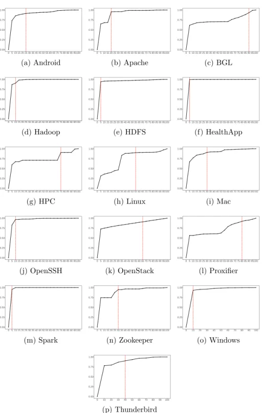
The x and y axes are in log scale. . . 31 5 The agreement ratio of log parsing results between using a part of log

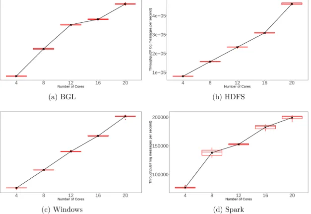
to generate dictionary and using all logs to generate dictionary. The red vertical lines indicate that the agreement ratios reach 90%. . . 32 6 Box plots of running time of Logram with different number of cores. . 33

(9)

List of Tables

1 Simplified log messages for illustration purposes. . . 6 2 The subject log data used in our evaluation. . . 21 3 Accuracy ofLogramcompared with other log parsers. The results that

are the highest among the parsers are annotaetd with * and the results that are higher than 0.9 are highlighted in bold. . . 22 4 The number of 2-grams and 3-grams in the dictionaries generated by

Logram . . . 26

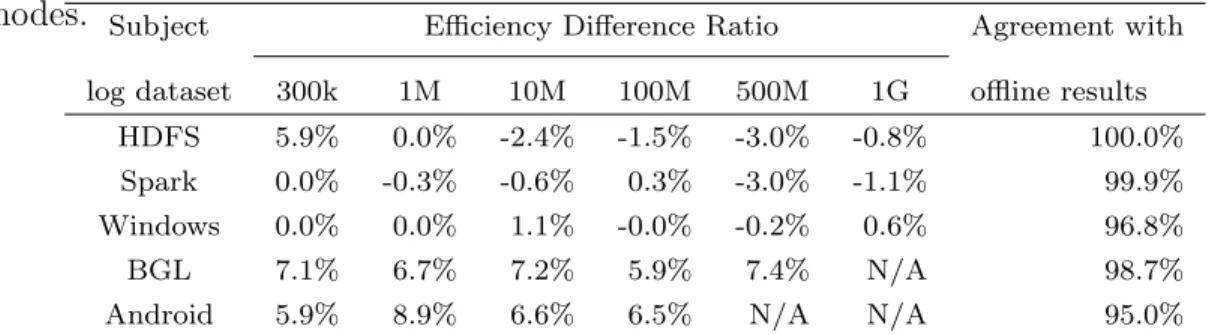
5 Comparing the parsing results ofLogrambetween the online and offline modes. . . 35

(10)

Chapter 1

Introduction

Modern software systems usually record valuable runtime information (e.g., impor-tant events and variable values) in logs. Logs play an imporimpor-tant role for practitioners to understand the runtime behaviors of software systems and to diagnose system failures [6, 14]. However, since logs are often very large in size (e.g., tens or hun-dreds of gigabytes) [56, 60], prior research has proposed automated approaches to analyze logs. These automated approaches help practitioners with various software maintenance and operation activities, such as anomaly detection [69, 70, 46, 25, 39], failure diagnosis [24, 2], performance diagnosis and improvement [51, 13], and system comprehension [24, 62]. Recently, the fast-emerging AIOps (Artificial Intelligence for IT Operations) solutions also depend heavily on automated analysis of operation logs [16, 44, 35, 23, 37].

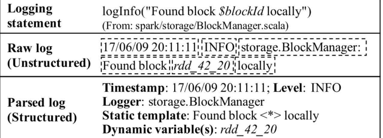
Logs are generated by logging statements in the source code. As shown in Fig-ure 1, a logging statement is composed of log level (i.e.,info), static text (i.e., “Found

block” and “locally”), and dynamic variables (i.e., “$blockId”). During system

run-time, the logging statement would generate raw log messages, which is a line of unstructured text that contains the static text and the values for the dynamic vari-ables (e.g., “rdd 42 20”) that are specified in the logging statement. The log message also contains information such as the timestamp (e.g., “17/06/09 20:11:11”) of when the event happened. In other words, logging statements define the templates for the log messages that are generated at runtime. Automated log analysis usually has difficulties analyzing and processing the unstructured logs due to their dynamic na-ture [69, 24]. Instead, a log parsing step is needed to convert the unstrucna-tured logs

(11)

17/06/09 20:11:11 INFO storage.BlockManager:

Found block

rdd

_

42

_

20

locally

Raw log

(Unstructured)

Logging

statement

logInfo("Found block

(From: spark/storage/BlockManager.scala)

$blockId

locally")

Timestamp

: 17/06/09 20:11:11;

Level

: INFO

Logger

: storage.BlockManager

Static template

: Found block <*> locally

Dynamic variable(s)

:

rdd

_

42

_

20

Parsed log

(Structured)

Figure 1: An illustrative example of parsing an unstructured log message into a structured format.

into a structured format before the analysis. The goal of log parsing is to extract the static template, dynamic variables, and the header information (i.e., timestamp, log level, and logger name) from a raw log message to a structured format. Such structured information is then used as input for automated log analysis. He et al. [29] found that the results of log parsing are critical to the success of log analysis tasks.

In practice, practitioners usually write ad hoc log parsing scripts that depend heavily on specially-designed regular expressions [75, 33, 38] . As modern software systems usually contain large numbers of log templates which are constantly evolv-ing [61, 72, 12], practitioners need to invest a significant amount of efforts to develop and maintain such regular expressions. In order to ease the pain of developing and maintaining ad hoc log parsing scripts, prior work proposed various approaches for automated log parsing [75]. For example, Drain [33] uses a fixed-depth tree to parse logs. Each layer of the tree defines a rule for grouping log messages (e.g., log mes-sage length, preceding tokens, and token similarity). At the end, log mesmes-sages with the same templates are clustered into the same groups. Zhu et al. [75] proposed a benchmark and thoroughly compared prior approaches for automated log parsing.

Despite the existence of prior log parsers, as the size of logs grows rapidly [40, 14, 6] and the need for low-latency log analysis increases [41, 37], efficiency becomes an important concern for log parsing. In this work, we proposeLogram, an automated log parsing approach that leveragesn-gram dictionaries to achieve efficient log parsing. In short,Logramuses dictionaries to store the frequencies ofn-grams in logs and leverage

(12)

then-gram dictionaries to extract the static templates and dynamic variables in logs. Our intuition is that frequentn-grams are more likely to represent thestatic templates

while rare n-grams are more likely to be dynamic variables. The n-gram dictionaries can be constructed and queried efficiently, i.e., with a complexity of O(n) and O(1), respectively.

We evaluatedLogramon 16 log datasets [75] and comparedLogramwith five state-of-the-art log parsing approaches. We found that Logram achieves a higher accuracy compared with the best existing approaches (i.e., at least 10% higher on average), and that Logram outperforms these best existing approaches in efficiency, achieving a parsing speed that is 1.8 to 5.1 times faster than the second-fastest approaches. Furthermore, as then-gram dictionaries can be constructed in parallel and aggregated efficiently, we demonstrated that Logram can achieve high scalability when deployed on a multi-core environment (e.g., a Spark cluster), without sacrificing any parsing accuracy. Finally, we demonstrated thatLogram can support effective online parsing, i.e., by updating the n-gram dictionaries continuously when new logs are added in a streaming manner.

In summary, the main contributions1 _{of our work include:}

• We present the detailed design of an innovative approach, Logram, for auto-mated log parsing. Logram leverages n-gram dictionaries to achieve accurate and efficient log parsing.

• We compare the performance of Logram with other state-of-the-art log parsing approaches, based on an evaluation on 16 log datasets. The results show that

Logramoutperforms other state-of-the-art approaches in efficiency and achieves

better accuracy than existing approaches.

• We deployedLogramonSpark and we show thatLogramscales out efficiently as the number ofSpark nodes increases (e.g., with near-linear scalability for some logs), without sacrificing paring accuracy.

• We demonstrate that Logram can effectively support online parsing, achieving similar parsing results and efficiency compared to the offline mode.

1_{The source code of our tool and the data used in our study are shared at}_{https://github.com/}

(13)

Our highly accurate, highly efficient, and highly scalableLogramcan benefit future research and practices that rely on automated log parsing for log analysis on large log data. In addition, practitioners can leverage Logram in a log streaming environment to enable effective online log parsing for real-time log analysis.

Thesis organization. The thesis is organized as follows. Section 2 introduces the

background of log parsing and n-grams. Section 3 surveys prior work related to log parsing. Section 4 presents a detailed description of our Logramapproach. Section 5 shows the results of evaluating Logram on 16 log datasets. Section 6 discusses the effectiveness of Logram for online log parsing. Section 7 discusses the threats to the validity of our findings. Finally, Section 8 concludes the thesis.

(14)

Chapter 2

Backgroud

In this section, we introduce the background of log parsing andn-grams that are used in our log parsing approach.

2.1

Log Parsing

In general, the goal of log parsing is to extract the static template, dynamic vari-ables, and the header information (i.e., timestamp, level, and logger) from a raw log message. While the header information usually follows a fixed format that is easy to parse, extracting the templates and the dynamic variables is much more challenging, because 1) the static templates (i.e., logging statements) that generate logs are usu-ally inaccessible [75], and 2) logs usuusu-ally contain a large vocabulary of words [38]. Table 1 shows four simplified log messages with their header information removed. These four log messages are actually produced from two static templates (i.e., “Found

block <*> locally” and “Dropping block <*> from memory”). These log messages

also contain dynamic variables (i.e., “rdd 42 20” and “rdd 42 22”) that vary across different log messages produced by the same template. Log parsing aims to separate the static templates and the dynamic variables from such log messages.

Traditionally, practitioners rely onad hocregular expressions to parse the logs that they are interested in. For example, two regular expressions (e.g., “Found block

[a-z0-9 ]+ locally” and “Dropping block [a-z0-9 ]+ from memory”) could be used to parse

the log messages shown in Table 1. Log processing & management tools (e.g.,Splunk1

(15)

Table 1: Simplified log messages for illustration purposes.

1. Found blockrdd 42 20 locally 2. Found blockrdd 42 22 locally

3. Dropping blockrdd 42 20 from memory 4. Dropping blockrdd 42 22 from memory

andELK stack2_{) also enable users to define their own regular expressions to parse log}

data. However, modern software systems usually contain large numbers (e.g., tens of thousands) of log templates which are constantly evolving [61, 72, 12, 42, 75]. Thus, practitioners need to invest a significant amount of efforts to develop and maintain

such ad hoc regular expressions. Therefore, recent work perform literature reviews

and study various approaches to automate the log parsing process [75, 22]. In this work, we propose an automated log parsing approach that is highly accurate, highly efficient, highly scalable, and supports online parsing.

2.2

n

-grams

An n-gram is a subsequence of length n from an item sequence (e.g., text [10], speech [64], source code [52], or genome sequences [66]). Taking the word sequence in the sentence: “The cow jumps over the moon” as an example, there are five 2-grams (i.e., bigrams): “The cow”, “cow jumps”, “jumps over”, “over the”, and “the moon”, and four 3-grams (i.e., trigrams): “The cow jumps”, “cow jumps over”, “jumps over the”, and “over the moon”. n-grams have been successfully used to model natural language [10, 43, 9, 11] and source code [36, 57, 53]. However, there exists no work that leverages n-grams to model log data. In this work, we propose Logram that leverages n-grams to parse log data in an efficient manner. Our intuition is that frequent n-grams are more likely to be static text while rare n-grams are more likely to be dynamic variables.

Logram extracts n-grams from the log data and store the frequencies of each n

-gram in dictionaries (i.e.,n-gram dictionaries). Finding all then-grams in a sequence (for a limitednvalue) can be achieved efficiently by a single pass of the sequence (i.e., with a linear complexity) [8]. For example, to get the 2-grams and 3-grams in the

(16)

sentence “The cow jumps over the moon”, an algorithm can move one word forward each time and get a 2-gram and a 3-gram starting from that word each time. Besides, the nature of the n-gram dictionaries enables one to construct the dictionaries in parallel (e.g., by building separate dictionaries for different parts of logs in parallel and then aggregating the dictionaries). Furthermore, the n-gram dictionaries can be updated online when more logs are added (e.g., in log streaming scenarios). As a result, as shown in our experimental results,Logramis highly efficient, highly scalable, and supports online parsing.

(17)

Chapter 3

Related Work

In this section, we discuss prior work that proposed log parsing techniques and prior work that leveraged log parsing techniques in various software engineering tasks (e.g., anomaly detection).

3.1

Prior Work on Log Parsing

In general, existing log parsing approaches could be grouped under three categories:

rule-based, source code-based, and data mining-based approaches.

Rule-based log parsing. Traditionally, practitioners and researchers hand-craft

heuristic rules (e.g., in the forms of regular expressions) to parse log data [68, 15, 28]. Modern log processing & management tools usually provide support for users to specify customized rules to parse their log data [58, 7, 19]. Rule-based approaches require substantial human effort to design the rules and maintain the rules as log formats evolve [61]. Using standardized logging formats [18, 1, 17] can ease the pain of manually designing log parsing rules. However, such standardized log formats have never been widely used in practice [38].

Source code-based log parsing. A log event is uniquely associated with a logging

statement in the source code (see Section 2.1). Thus, prior studies proposed auto-mated log parsing approaches that rely on the logging statements in the source code to derive log templates [69, 50]. Such approaches first use static program analysis to extract the log templates (i.e., from logging statements) in the source code. Based on the log templates, these approaches automatically compose regular expressions

(18)

to match log messages that are associated with each of the extracted log templates. Following studies [71, 59] applied [69] on production logs (e.g., Google’s production logs) and achieved a very high accuracy. However, source code is often not available for log parsing tasks, for example, when the log messages are produced by closed-source software or third-party libraries; not to mention the efforts for performing static analysis to extract log templates using different logging libraries or different programming languages.

Data mining-based log parsing. Other automated log parsing approaches do

not require the source code, but instead, leverage various data mining techniques.

SLCT [67], LogCluster [49], and LFA [49] proposed approaches that automatically parse log messages by mining the frequent tokens in the log messages. These ap-proaches count token frequencies and use a predefined threshold to identify the static components of log messages. The intuition is that if a log event occurs many times, then the static components will occur many times, whereas the unique values of the dynamic components will occur fewer times. Prior work also formulated log parsing as a clustering problem and used various approaches to measure the similarity/distance between two log messages (e.g.,LKE [25],LogSig [65],LogMine [27],SHISO [48], and

LenMa [63]). For example, LKE [25] clusters log messages into event groups based

on the edit distance, weighted by token positions, between each pair of log messages.

AEL [38] used heuristics based on domain knowledge to recognize dynamic com-ponents (e.g., tokens following the “=” symbol) in log messages, then group log messages into the same event group if they have the same static and dynamic com-ponents. Spell [20] parses log messages based on a longest common subsequence algorithm, built on the observation that the longest common subsequence of two log messages are likely to be the static components. IPLoM [47] iteratively partitions log messages into finer groups, firstly by the number of tokens, then by the position of to-kens, and lastly by the association between token pairs. Drain [33] uses a fixed-depth tree to represent the hierarchical relationship between log messages. Each layer of the tree defines a rule for grouping log messages (e.g., log message length, preceding tokens, and token similarity). Zhu et al. [75] evaluated the performance of such data mining-based parsers and they found that Drain [33] achieved the best performance in terms of accuracy and efficiency. Our n-gram-based log parser achieves a much faster parsing speed and a better parsing accuracy compared to Drain.

(19)

In addition, prior study performed a systematic literature review on automated log parsing techniques [22]. They investigated the advantages and limitations of 17 log parsing techniques in terms of seven aspects, such as efficiency and required parameter tuning effort, which can help practitioners choose the right log parsers for their specific scenarios and provide insights for future research directions.

3.2

Applications of Log Parsing

Log parsing is usually a prerequisite for various log analysis tasks, such as anomaly detection [69, 70, 46, 25, 39], failure diagnosis [24, 2], performance diagnosis and improvement [51, 13], and system comprehension [24, 62]. For example, Fu et al. [25] first parse the raw log messages to extract log events. Based on the extracted event sequences, they then learn a Finite State Automaton (FSA) to represent the normal work flow, which is in turn used to detect anomalies in new log files. Prior work [29] shows that the accuracy of log parsing is critical to the success of log analysis tasks. Besides, as the size of log files grows fast [40, 14, 6], a highly efficient log parser is important to ensure that the log analysis tasks can be performed in a timely manner. In this work, we propose a log parsing approach that is not only accurate but also efficient, which can benefit future log analysis research and practices.

(20)

Chapter 4

Approach

In this section, we present our automated log parsing approach that is designed using

n-gram dictionaries.

4.1

Overview of

Logram

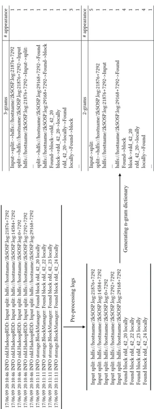
Our approach consists of two steps: 1) generatingn-gram dictionaries and 2) parsing log messages usingn-gram dictionaries. In particular, the first step generatesn-grams from log messages and calculate the number of appearances of each n-gram. In the second step, each log message is transformed into n-grams. By checking the number of appearance of eachn-gram, we can automatically parse the log message into static text and dynamic variables. Figure 2 and 3 show the overview of our approach with a running example.

4.2

Generating an

n

-gram dictionary

4.2.1

Pre-processing logs

In this step, we extract a list of tokens (i.e., separated words) from each log message. First of all, we extract the content of a log message by using a pre-defined regular expression. For example, a log message often starts with the time stamp , the log level, and the logger name. Since these parts of logs often follow a common format in the same software system (specified by the configuration of logging libraries), we can directly parse and obtain these information. For example, a log message from the

(21)

running example in Figure 2, i.e., “17/06/09 20:11:11 INFO storage.BlockManager:

Found block rdd 42 24 locally”, “17/06/09 20:11:11” is automatically identified as

time stamp, “INFO” is identified as the log level and “Storage.BlockManager:” is identified as the logger name; while the content of the log is “Found block rdd 42 24

locally”. After getting the content of each log message, we split the log message into

tokens. The log message is split with white-space characters (e.g., space and tab). Finally, there exist common formats for some special dynamic information in logs, such as IP address and email address.

In order to have a unbiased comparison with other existing log parsers in the

LogPai benchmark (cf. Section 5), we leverage the openly defined regular expressions

that are available from the LogPai benchmark to identify such dynamic information.

4.2.2

Generating an

n-gram dictionary

We use the log tokens extracted from each log message to create ann-gram dictionary. Naively, for a log message with m tokens, one may create an n-gram where n ≤ m. However, when m has the same value as n, the phrases with n-grams are exactly all log messages. Such a dictionary is not useful since almost all log messages have tokens that are generated from dynamic variables. On the other hand, a small value of n

may increase the chance that the text generated by a dynamic variable has multiple appearances. A prior study [30] finds that the repetitiveness of an n-gram in logs starts to become stable when n ≤ 3. Therefore, in our approach, we generate the dictionary using phrases with two or three words (i.e., 2-grams and 3-grams). Naively, one may generate the dictionary by processing every single log message independently. However, such a naive approach has two limitations: 1) some log events may span across multiple lines and 2) the beginning and the ending tokens of a log message may not reside in the same number of n-grams like other tokens (c.f. our parsing step “Identifying dynamically and statically generated tokens” in Section 4.3.2). For example, the first token of each log message cannot be put in a 2-gram nor 3-gram and the second token of each log line cannot be put in a 3-gram. This limitation may lead to potential bias of the tokens being considered as dynamic variables. In order to ensure that all the tokens are considered equally when generating the n -gram dictionary forLogram, at the beginning and the ending tokens of a log message, we also include the end of the prior log message and the beginning of the following

(22)

log message, respectively, to create n-grams. For example, if our highest n in the

n-gram is 3, we would check two more tokens at the end of the prior log message and the beginning of the following log message. In addition, we calculate the number of occurrences of each n-gram in our dictionary.

As shown in a running example in Figure 2, a dictionary from the nine lines of logs is generated consisting of 3-grams and 2-grams. Only one 3-grams, “

locally->Found->block”, in the example have multiple appearance. Three 2-grams, “

Found->block”, “Input->split:” and “locally->Found”, have four to five appearances. In

particular, there exists n-grams, such as the 3-gram “locally->Found->block”, that are generated by combining the end and beginning of two log messages. Without such combination, tokens like “input”, “Found” and “locally” will have lower appearance in the dictionary.

4.3

Parsing log messages using an

n

-gram

dictio-nary

In this step of our approach, we parse log messages using the dictionary that is generated from the last step.

4.3.1

Identifying

n-grams that may contain dynamic

vari-ables

Similar to the last step, each log message is transformed into n-grams. For each

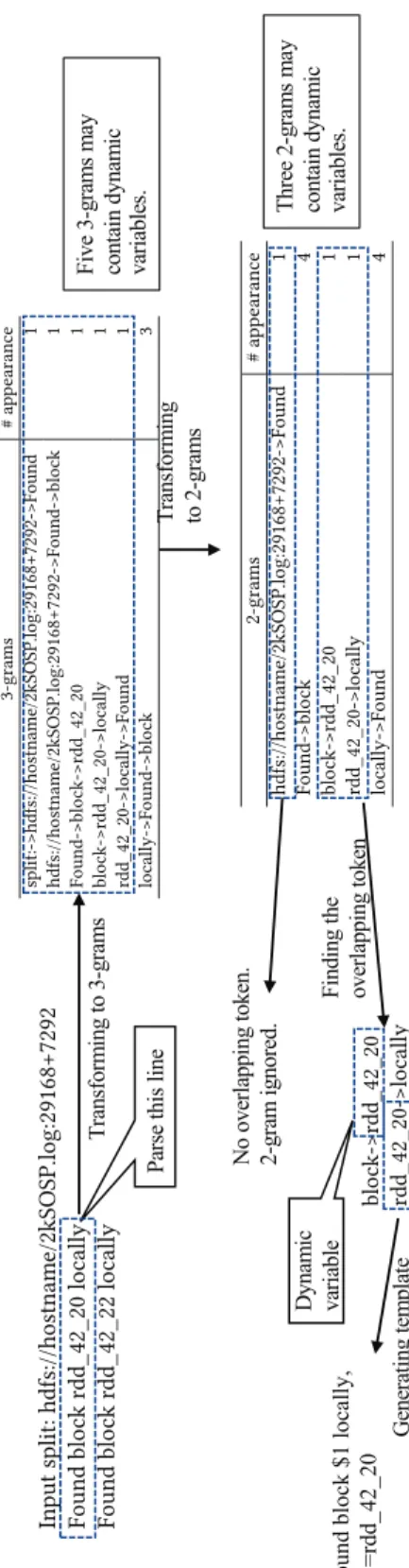
n-gram from the log message, we check its number of appearances in the dictionary. If the number of occurrence of a n-gram is smaller than a automatically determined threshold (see Section 4.3.3), we consider that the n-gram may contain a token that is generated from dynamic variables. In order to scope down to identify the dynami-cally generated tokens, after collecting all low-appearing n-grams, we transform each of thesen-grams inton−1-grams, and check the number of appearance of eachn− 1-gram. We recursively apply this step until we have a list of low-appearing 2-grams, where each of them may contain one or two tokens generated from dynamic variables. For our running example shown in Figure 3, we first transform the log message into two 3-grams, while both only have one appearance in the dictionary. Hence, both

(23)

3-grams from the running example in Figure 3 may contain dynamic variables. Af-terwards, we transform the 3-grams into three 2-grams. One of the 2-grams (“

Found->block”) has four appearances; while the other two 2-grams (“block->rdd 42 20” and

“rdd 42 20->locally”) only have one appearance. Therefore, we keep the two 2-grams

to identify the dynamic variables.

4.3.2

Identifying dynamically and statically generated

to-kens

From the last step, we obtain a list of low-appearing 2-grams. However, not all tokens in the 2-grams are dynamic variables. There may be 2-grams that have only one dynamically generated token while the other token is static text. In such cases, the token from the dynamic variable must reside in two consecutive low-appearing 2-grams (i.e., one ends with the dynamic variable and one starts with the dynamic variable). For all other tokens, including the ones that are now selected in either this step or the last step, we consider them as generated from static text.

However, a special case of this step is the beginning and ending tokens of each log message (c.f. the previous step “Generating ann-gram dictionary” in Section 4.2.2). Each of these tokens would only appear in smaller number of n-grams. For example, the first token of a log message would only appear in one 2-gram. If these tokens of the log message are from static text, they may be under-counted to be considered as potential dynamic variables. If these tokens of the log message are dynamically gen-erated, they would never appear in two 2-grams to be identified as dynamic variable. To address this issue, for the beginning and ending tokens of each log message, we generate additionaln-grams by considering the ending tokens from the prior log mes-sage; and for the ending tokens of each log message, we generate additional n-grams by considering the beginning tokens from the next log message.

For our running example shown in Figure 3, “rdd 42 20” is generated from dy-namic variable and it reside in two 2-grams (“block->rdd 42 20” and “rdd 42

20->locally”. Therefore, we can identify token “rdd 42 20” as a dynamic variable, while

“block” and “locally” are static text. On the other hand, since “hdfs://hostname/2kSOSP.log

:29168+7292->Found” only appear without overlapping tokens with others, we

ig-nore this 2-gram for identifying dynamic variables.

(24)

tokens. For example, if we have three tokens that form a 3-gram dynamic->

static->dynamic, when transforming the 3-gram, we end up with two 2-grams:

dynamic->static andstatic->dynamic. Both 2-grams would be low-appearing 2-grams as both

of them include a dynamic token. As the token static appears in two low-appearing 2-grams, it would be falsely identified as a dynamic token based on our earlier rule. In order to cope with such special cases, when a token is surrounded by two dynamic tokens, we create a pseudo bi-gram using a wildcard (e.g., ?->static), and use its frequency to determine whether the middle token (e.g., static) is static or dynamic.

4.3.3

Automatically determining the threshold of

n-gram

oc-currences

The above identification of dynamically and statically generated tokens depends on a threshold of the occurrences of n-grams. In order to save practitioners’ effort for manually searching the threshold, we use an automated approach to estimate the appropriate threshold. Our intuition is that most of the static n-grams would have more occurrences while the dynamic n-grams would have fewer occurrences. There-fore, there may exist a gap between the occurrences of the static n-grams and the occurrences of the dynamicn-grams, i.e., such a gap helps us identify a proper thresh-old automatically.

In particular, first, we measure the occurrences of each n-gram. Then, for each occurrence value, we calculate the number ofn-grams that have the exact occurrence value. We use a two-dimensional coordinate to represent the occurrence values (i.e., the X values) and the number ofn-grams that have the exact occurrence values (i.e., theY values). Then we use theloess function [5] to smooth theY values and calculate the derivative of theY values against theX values. After getting the derivatives, we use Ckmeans.1d.dp [3], a one-dimensional clustering method, to find a break point to separate the derivatives into two groups, i.e., a group for static n-grams and a group for dynamicn-grams. The breaking point would be automatically determined as the threshold.

(25)

4.3.4

Generating log templates

Finally, we generate log templates based on the tokens that are identified as dynam-ically or statdynam-ically generated. We follow the same log template format as the LogPai

benchmark [75], in order to assist in further research. For our running example shown in Figure 3, our approach parses the log message “Found block rdd 42 20 locally” into

(26)

17/06/09 20:10:46 INFO rdd.Hado opRDD: Input split: hdfs://hostname/2kSOSP .log:21876+7292 17/06/09 20:10:46 INFO rdd.Hado opRDD: Input split: hdfs://hostname/2kSOSP .log:14584+7292 17/06/09 20:10:46 INFO rdd.Hado opRDD: Input split: hdfs://hostname/2kSOSP .log:0+7292 17/06/09 20:10:46 INFO rdd.Hado opRDD: Input split: hdfs://hostname/2kSOSP .log:7292+7292 17/06/09 20:10:46 INFO rdd.Hado opRDD: Input split: hdfs://hostname/2kSOSP .log:29168+7292 17/06/09 20:11:11 INFO storage .Blo ckManager: Found blo ck rdd_42_20 lo cally 17/06/09 20:11:11 INFO storage .Blo ckManager: Found blo ck rdd_42_22 lo cally 17/06/09 20:11:11 INFO storage .Blo ckManager: Found blo ck rdd_42_23 lo cally 17/06/09 20:11:11 INFO storage .Blo ckManager: Found blo ck rdd_42_24 lo cally Input split: hdfs://hostname/2kSOSP .log:21876+7292 Input split: hdfs://hostname/2kSOSP .log:14584+7292 Input split: hdfs://hostname/2kSOSP .log:0+7292 Input split: hdfs://hostname/2kSOSP .log:7292+7292 Input split: hdfs://hostname/2kSOSP .log:29168+7292 Found blo ck rdd_42_20 lo cally Found blo ck rdd_42_22 lo cally Found blo ck rdd_42_23 lo cally Found blo ck rdd_42_24 lo cally ! !"" " !# ! #!& 3-grams # app earance Input->split:->hdfs://hostname/2kSOSP .log:21876+7292 1 split:->hdfs://hostname/2kSOSP .log:21876+7292->Input 1 hdfs://hostname/2kSOSP .log:21876+7292->Input->split: 1 ... 1 split:->hdfs://hostname/2kSOSP .log:29168+7292->Found 1 hdfs://hostname/2kSOSP .log:29168+7292->Found->blo ck 1 Found->blo ck->r dd_42_20 1 blo ck->r dd_42_20->lo cally 1 rdd_42_20->lo cally->Found 1 lo cally->Found->blo ck 3 ... 1 2-grams # app earance Input->split: 5 split:->hdfs://hostname/2kSOSP .log:21876+7292 1 hdfs://hostname/2kSOSP .log:21876+7292->Input 1 ... 1 hdfs://hostname/2kSOSP .log:29168+7292->Found 1 Found->blo ck 4 blo ck->r dd_42_20 1 rdd_42_20->lo cally 1 lo cally->Found 4 ... 1

Figure 2: A running example of generating n-gram dictionary, which will be later used for parsing each log messages as shown in Figure 3.

(27)

2-grams # app earance hdfs://hostname/2kSOSP .log:29168+7292->Found 1 Found->blo ck 4 blo ck->r dd_42_20 1 rdd_42_20->lo cally 1 lo cally->Found 4 3-grams # app earance split:->hdfs://hostname/2kSOSP .log:29168+7292->Found 1 hdfs://hostname/2kSOSP .log:29168+7292->Found->blo ck 1 Found->blo ck->r dd_42_20 1 blo ck->r dd_42_20->lo cally 1 rdd_42_20->lo cally->Found 1 lo cally->Found->blo ck 3 ! ! " & # & %! " & %! Input split: hdfs://hostname/2kSOSP .log:29168+7292 Found blo ck rdd_42_20 lo cally Found blo ck rdd_42_22 lo cally blo ck->r dd_42_20 rdd_42_20->lo cally !" ! # ! " % ! " & # & %! " !" ! # ! " # %! # ! # # # $ & ! !" # " %! # ! !

Figure 3: A running example of parsing one log message using the dictionary built from Figure 2.

(28)

Chapter 5

Evaluation

In this section, we present the evaluation of our approach. We evaluate our approach by parsing logs from theLogPai benchmark [75]. We compareLogramwith five auto-mated log parsing approaches, includingDrain [33], Spell [20], AEL [38],Lenma [63]

andIPLoM [47] that are from prior research and all have been included in the LogPai

benchmark. We choose these five approaches since a prior study [75] finds that these approaches have the highest accuracy and efficiency among all of the evaluated log parsers. In particular, we evaluate our approach on four aspects:

Accuracy. The accuracy of a log parser measures whether it can correctly identify

the static text and dynamic variables in log messages, in order to match log messages with the correct log events. A prior study [29] demonstrates the importance of high accuracy of log parsing, and low accuracy of log parsing can cause incorrect results (such as false positives) in log analysis.

Efficiency. Large software systems often generate a large amount of logs during run

time [54]. Since log parsing is typically the first step of analyzing logs, low efficiency in log parsing may introduce additional costs to practitioners when doing log analysis and cause delays to uncover important knowledge from logs.

Ease of stabilisation. Log parsers typically learn knowledge from existing logs in

order to determine the static and dynamic components in a log message. The more logs seen, the better results a log parser can provide. It is desired for a log parser to have a stable result with learning knowledge from a small amount of existing logs, such that parsing the log can be done in a real-time manner without the need of updating knowledge while parsing logs.

(29)

Scalability. Due to the large amounts of log data, one may consider leveraging parallel processing frameworks, such as Hadoop and Spark, to support the parsing of logs [31]. However, if the approach of a log parser is difficult to scale, it may not be adopted in practice.

5.1

Subject log data

We use the data set from theLogPai benchmark [75]. The data sets and their descrip-tions are presented in Table 2. The benchmark includes logs produced by both open source and industrial systems from various domains. These logs are typically used as subject data for prior log analysis research, such as system anomaly detection [34, 45], system issue diagnosis [21] and system understanding [55]. To assist in automatically calculating accuracy on log parsing (c.f., Section 5.2), each data set in the benchmark includes a subset of 2,000 log messages that are already manually labeled with log event. Such manually labeled data are used in evaluating the accuracy of our log parser. For the other three aspects of the evaluation, we use the entire logs of each log data set.

5.2

Accuracy

In this subsection, we present the evaluation results on the accuracy of Logram. Prior approach by Zhu et al. [75] defines an accuracy metric as the ratio of correctly parsed log messages over the total number of log messages. In order to calculate the parsing accuracy, a log event template is generated for each log message and log messages with the same template will be grouped together. If all the log messages that are grouped together indeed belong to the same log template, and all the log messages that indeed belong to this log template are in this group, the log messages are considered parsed correctly. However, the grouping accuracy has a limitation that it only determines whether the logs from the same events are grouped together; while the static text and dynamic variables in the logs may not be correctly identified. We discuss the limitation of using the grouping accuracy in detail in the Results

subsection.

(30)

Table 2: The subject log data used in our evaluation.

Dataset

Description

Size

Android

Android framework log

183.37MB

Apache

Apache server error log

4.90MB

BGL

Blue Gene/L supercomputer log

708.76MB

Hadoop

Hadoop mapreduce job log

48.61MB

HDFS

Hadoop distributed file system log

1.47GB

HealthApp

Health app log

22.44MB

HPC

High performance cluster log

32.00MB

Linux

Linux system log

2.25MB

Mac

Mac OS log

16.09MB

OpenSSH

OpenSSH server log

70.02MB

OpenStack

OpenStack software log

58.61MB

Proxifier

Proxifier software log

2.42MB

Spark

Spark job log

2.75GB

Thunderbird

Thunderbird supercomputer log

29.60GB

Windows

Windows event log

26.09GB

Zookeeper

ZooKeeper service log

9.95MB

are indeed important for various log analysis. For example, Xu et al. [69] consider the variation of the dynamic variables to detect run-time anomalies. Therefore, we manually check the parsing results of each log message and determine whether the static text and dynamic variables are correctly parsed, i.e., parsing accuracy. In other words, a log message is considered correctly parsed if and only if all its static text and dynamic variables are correctly identified.

Results

(31)

Table 3: Accuracy of Logram compared with other log parsers. The results that are the highest among the parsers are annotaetd with * and the results that are higher than 0.9 are highlighted in bold.

Dataset Drain AEL Lenma Spell IPLoM Logram

Android 0.933 0.867 0.976* 0.933 0.716 0.848 Apache 0.693 0.693 0.693 0.693 0.693 0.699* BGL 0.822* 0.818 0.577 0.639 0.792 0.740 Hadoop 0.545 0.539 0.535 0.192 0.373 0.965* HDFS 0.999* 0.999* 0.998 0.999* 0.998 0.981 HealthApp 0.609 0.615 0.141 0.602 0.651 0.969* HPC 0.929 0.990* 0.915 0.694 0.979 0.959 Linux 0.250 0.241 0.251 0.131 0.235 0.460* Mac 0.515 0.579 0.551 0.434 0.503 0.666* OpenSSH 0.507 0.247 0.522 0.507 0.508 0.847* Openstack 0.538 0.718 0.759* 0.592 0.697 0.545 Proxifier 0.973* 0.968 0.955 0.785 0.975 0.951 Spark 0.902 0.965* 0.943 0.865 0.883 0.903 Thunderbird 0.803 0.782 0.814* 0.773 0.505 0.761 Windows 0.983* 0.983* 0.277 0.978 0.554 0.957 Zookeeper 0.962 0.922 0.842 0.955 0.967* 0.955 Average 0.748 0.745 0.672 0.669 0.689 0.825*

of the 16 log datasets. Table 3 shows the accuracy on 16 datasets. Following the

prior log-parsing benchmark [75], we highlight the accuracy values that are higher than 0.9 or that are the highest for each log dataset. Logram achieves an average parsing accuracy of 0.825, which is at least 10% higher than the average accuracy achieved by any other log parsers. The second most accurate approach, i.e., Drain, achieves an average parsing accuracy of 0.748. For eight log datasets, Logram has an parsing accuracy higher than 0.9; for four other datasets, Logram has the highest parsing accuracy among all parsers. Since Logram is designed based on processing every token in a log instead of comparing each line of logs with others,Logramexceeds other approaches in terms of parsing accuracy.

Even though prior approaches may often correctly group log messages together, the static text and dynamic variables of these log messages may not be correctly identi-fied. For example, when parsing the Hadoop logs, the parserSpell achieves a grouping accuracy of 0.778 [75] but the parsing accuracy is only 0.192. By manually checking

(32)

the results, we find that some groups of logs share the same strings of host names that are generated from dynamic variables but are parsed as static tokens. For exam-ple, a log message “Address change detected. Old: msra-sa-41/10.190.173.170:9000

New: msra-sa-41:9000” is parsed into a log template “Address change detected. Old

msra-sa-41/<*> <*>New msra-sa-41<*>”. We can see that the strings “msra-sa”

and “msra-sa-41” in the host names are not correctly detected as dynamic variables. However, since all the log messages in this category have such strings in the host names, even thoughSpell cannot identify the dynamic variables, the log messages are still grouped together. In particular, we manually examined the parsing results of

Logram for all the log lines that are considered to be correctly parsed in terms of the

grouping accuracy [75]. In total, we found that 17.8% (4641 out of 26017) of the log lines that are considered to be correctly parsed in terms of the grouping accuracy are actually incorrectly parsed based on our manual examination. For each log file, 0.2% to 79.2% of the log lines that are considered correctly parsed in terms of the grouping accuracy are false positives.

Finally, we manually study the incorrectly parsed log messages by Logram. Such incorrectly parsed log messages can be due to false-dynamic, i.e., a static token that is identified as a dynamic token, or false-static, i.e., a dynamic token that is mis-identified as a static token. For all the lines that are incorrectly parsed, 41.1% contain false-dynamic tokens and 61.8% contain false-static tokens. Through further manual investigation, we identify the following three reasons of incorrectly parsing some of the log messages:

1. Mis-split tokens. Some log messages contain special tokens such as + and{to

separate two tokens. In addition, sometimes static text and dynamic variables are printed into one single token without any separator (like a white space). It is difficult for a token-based approach to address such cases. This reason may contribute to both false-static and false-dynamic results.

2. Pre-processing errors. The pre-processing of common log formats may

in-troduce mistakes to the log parsing. For example, text in a common format (e.g., a date format) may be part of a long dynamic variable (a task id with its date as part of it). However, the pre-processing step extracts only the text in the common format, causing the rest of the text in the dynamic variable being parsed into a wrong format. This reason may contribute to false-static results.

(33)

3. Frequently-appearing dynamic variables. Some dynamic variables contain contextual information of system environment and can appear frequently in logs. For example, in Apache logs, the path to a property file often appears in log messages such as: “workerEnv.init() ok /etc/httpd/conf/workers2.properties”. Although the path is a dynamic variable, in fact, the value of the dynamic variable never changes in the logs, preventing Logram from identifying it as a dynamic variable. On the other hand, such an issue is not challenging to address in practice. Practitioners can consider such contextual information in the pre-processing step.

5.3

Efficiency

To measure the efficiency of a log parser, similar to prior research [32, 75], we record the elapsed time to finish the entire end-to-end parsing process on different log data with varying log sizes. The elapsed time one of the important metrics included in the ISO-25010 [4]. Among other metrics that also indicate efficiency, such as resource utilization, elapsed time is important for a log parser as log parsing is the first step in automated log analysis, any delay would impact the entire pipeline of log analysis. We randomly extract data chunks of different sizes, i.e., 300KB, 1MB, 10MB, 100MB, 500MB and 1GB. Specifically, we choose to evaluate the efficiency from the Android, BGL, HDFS, Windows and Spark datasets, due to their proper sizes for such eval-uation. From each log dataset, we randomly pick a point in the file and select a data chunk of the given size (e.g., 1MB or 10MB). We ensure that the size from the randomly picked point to the end of the file is not smaller than the given data size to be extracted. We measure the elapsed time for the log parsers on a desktop computer with Inter Core i5-2400 CPU 3.10GHz CPU, 8GB memory and 7,200rpm SATA hard drive running Ubuntu 18.04.2. We compare Logram with three other parsers, i.e., Drain, Spell and AEL, that all have high accuracy in our evaluation and more importantly, have the highest efficiency on log parsing based on the prior benchmark study [75].

In addition, we calculate the size of the dictionaries that are generated by Logram

(cf. Section 4.2). These dictionaries are meant to be kept in memory to assist in a fast parsing of logs. The large size of the dictionaries may become a memory overhead

(34)

to the efficiency of the approach.

Results

Logramoutperforms the fastest state-of-the-art log parsers in efficiency by

1.8 to 5.1 times. Figure 4 shows that time needed to parse five different log data

with various sizes using Logramand five other log parsers. We note that for Logram, the time to construct the dictionaries is already included in our end-to-end elapsed time, in order to fairly compare log parsing approaches. The dictionary construction (including pre-processing log messages and generating n-gram dictionaries) accounts for 77% to 92% of the overall parsing time, while parsing the log messages using the constructed dictionaries only takes 8% to 23% of the overall parsing time. We find

that Logram drastically outperform all other existing parsers. In particular, Logram

is 1.8 to 5.1 times faster than the second fastest approaches when parsing the five log datasets along different sizes.

The efficiency ofLogramis stable when increasing the sizes of logs. From

our results, the efficiency of Logram is not observed to be negatively impacted when the size of logs increases. For example, the running time only increases by a factor of 773 to 1039 when we increase the sizes of logs from 1 MB to 1GB (i.e., by a factor of 1,000). Logram keeps a dictionary that is built from the n-grams in log messages. With larger size of logs, the size of dictionary may drastically increasing. However, our results indicate that up to the size of 1GB of the studied logs, the efficiency keeps stable. We consider the reason is that when paring a new log message using the dictionary, the look-up time for ann-gram in our dictionary is consistent, despite the size of the dictionary. Hence even with larger logs, the size of the dictionary do not drastically change.

On the other hand, the efficiency of other log parsers may deteriorate with larger logs. In particular, Lenma has the lowest efficiency among all studied log parsers.

Lenma cannot finish finish parsing any 500MB and 1GB log dataset within hours.

In addition, Spell would crash on Windows and Spark log files with 1G size due to memory issues. AEL shows a lower efficiency when parsing large Windows and BGL logs. Finally, Drain, although not as efficient as Logram, does not have a lower efficiency when parsing larger sizes of logs, which agrees with the finding in prior research on the log parsing benchmark [75].

(35)

Logramdoes not generate large size of dictionaries as memory overhead.

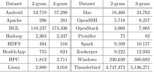
Table 4 shows the sizes of both 2-gram and 3-gram dictionaries that are generated by each log dataset. We found that, a dataset with a large dictionary, e.g, BGL, has less than 300K keys in total, which only takes 11.2 MB (4.1MB for 2-grams and 7.1MB for 3-grams) of memory. The largest dataset, i.e., the Thunderbird logs, has a total of nearly 9 million keys. However, the dictionary only takes 412 MB (150 MB for 2-grams and 262 MB for 3-grams) of memory. On the other hand, we also found that a large log dataset may not have as large a dictionary. For example, the Windows logs have almost a similar size as the Thunderbird logs but the generated dictionary only has 600K keys, which is only 7% of the size of the dictionary generated from the Thunderbird logs. Our results show that the size of the dictionaries may be influenced not only by the size of the logs, but also by other characteristics of the logs (e.g., the number of unique 2-grams and 3-grams).

Table 4: The number of 2-grams and 3-grams in the dictionaries generated byLogram

Dataset

2-gram

3-gram

Dataset

2-gram

3-gram

Android

53,719

57,298

Mac

18,460

24,762

Apache

296

281

OpenSSH

5,718

9,257

BGL

110,237

174,336

OpenStack

3,960

7,865

Hadoop

2,363

2,337

Proxifier

75

82

HDFS

494

516

Spark

9,169

10,157

HealthApp

755

624

Zookeeper

9,222

12,933

HPC

1,813

2,711

Windows

230,639

380,682

Linux

2,880

3,016

Thunderbird

3,747,372

5,136,271

5.4

Ease of stabilisation

We evaluate the ease of stabilisation by runningLogrambased on the dictionary from a subset of the logs. In other words, we would like to answer the following question:

Can we generate a dictionary from a small size of log data and correctly parse the rest of the logs without updating the dictionary?

(36)

If so, in practice, one may choose to generate the dictionary with a small amount of logs without the need of always updating the dictionary while parsing logs, in order to achieve even higher efficiency and scalability. In particular, for each subject log data set, we first build the dictionary based on the first 5% (or 10% only for large datasets like Thunderbird and Windows) of the entire logs. Then we use the dictionary to parse the entire log data set. Due to the limitation of grouping accuracy found from the last subsection and the limitation of the high human effort needed to manually calculate the parsing accuracy, we do not calculate any accuracy for the parsing results. Instead, we automatically measure the agreement between the parsing result using the dictionary generated from the first 5% (or 10%) lines of logs and the entire logs. For each log message, we only consider that the two parsing results agree to each other if they are exactly the same. We then gradually increase the size of logs to build a dictionary by appending another 5% (or 10%) of logs. We keep calculating the agreement until the agreement is 100%.

Results

Logram achieves stable parsing results using a dictionary generated from

a small portion of log data. Figure 5 shows agreement ratio between parsing

results from using partial log data to generate ann-gram dictionary and using all log data. The red line in the figures indicates that the agreement ratio is over 90%. In 10 out of 16 studied log data sets, our log parser can generate ann-gram dictionary from less than 30% of the entire log data, while having over 90% of the log parsing results the same as using all the logs to generate a dictionary. In particular, one of the large log datasets (the Spark logs) gains a 95.5% agreement ratio using only the first 5% of the log data to build the dictionary. Our results show that the log data is indeed repetitive. Such results demonstrate that practitioners can consider leveraging the two parts ofLogram separately, i.e., generating the n-gram dictionary (i.e., Figure 2) may not be needed for every log message, while the parsing of each log message (i.e., Figure 3) can depend on a dictionary generated from existing logs.

We manually check the other six log datasets and we find three reasons that that may cause the instability. 1) Some parts of the log datasets have drastically different log events than others. For example, between the first 30% and 35% of the log data in Linux, a large number of log messages are associated with new events for

(37)

Bluetooth connections and memory issues. Such events do not exist in the logs in the beginning of the dataset. The unseen logs cause parsing results using dictionary from the beginning of the log data to be less agreed with the parsing results using the the entire logs. However, it is interesting to see that after our dictionary learns the

n-grams in that period, the log parsing results become stable. Therefore, in practice, developers may need to monitor the parsing results to determine the need of updating the n-gram dictionary from logs. 2) Log data is too small to reach stabilisation. For example, Proxifier has a very small dataset of logs (only 2.42MB). By using even a smaller part of logs (as small as 5%) to generate the dictionary, the dictionary may have a low coverage of the n-grams in the entire dataset, making it difficult to reach stabilisation when the size of the logs used to generated the dictionary is small. 3) The inaccurate parsing results resulted from mis-split tokens may also lead to instability in our results. When tokens are not split correctly, it may lead to the gradual increase of new n-grams in the dictionary. For example, for OpenStack, we observed a steady increase of the number ofn-grams when we increase the size of the dataset to build the dictionaries, which is due to mis-split tokens. In fact, the parsing accuracy of OpenStack is almost the worst among all the datasets (shown in Table 3). As using a smaller part of the logs would generate dictionaries that cannot represent a sufficient coverage of all the n-grams in the dataset, it is difficult to achieve an early stabilisation.

5.5

Scalability

In order to achieve a high-scalability of log parsing, we migrate Logram to Spark.

Spark [73] is an open-source distributed data processing engine, with high-level API

in several program languages such as Java, Scala, Python, and R. Spark has been adopted widely in practice for analyzing large-scale data including log analysis. We migrate each step ofLogram, i.e., 1) generatingn-gram model based dictionaries and 2) parsing log messages using dictionaries, separately to Spark. In particular, the first step of generating dictionary is written similar as a typicallywordcount example program, where each item in the dictionary is a n-gram from a log message. In addition, the second step of parsing log messages is trivial to run in parallel where

(38)

each log message is parsed independently1_.

We evaluate the scalability of Logram on a clustering with one master node and five worker nodes running Spark 2.43. Each node is deployed on a desktop machine with the same specifications as used in our efficiency evaluation (cf. Section 5.3). In total, our cluster has four cores for each worker, leading to a total of 20 cores for processing logs. We first store the log data into HDFS that are deployed on the cluster with a default option of three replications. We then run the Spark based Logram on

the Spark cluster with one worker (four cores) to five workers (20 cores) enabled. We

evaluate the scalability on the same log datasets used for evaluating the efficiency, except for Android due to its relatively small size. We measure the throughput for parsing each log data to assess scalability. Due to the possible noise in a local network environment and the indeterministic nature of the parallel processing framework, we independently repeat each run 10 times when measuring throughput, i.e., number of log messages parsed per second.

Results

Logram scales out efficiently with the number of Spark nodes without

sacrificing parsing accuracy. Figure 6 uses boxplots to present the throughput

(i.e., number of log messages parsed per second) of Logram when we increase the number of nodes from one (i.e., four cores) to five (i.e., 20 cores).As shown in Figure 6, the throughput increases nearly linearly, achieving up to 5.7 times speedup as we increase the number of nodes by a factor of five. In addition, Figure 6 shows that the throughput of Logram has low variance when we repeat the parsing of each log dataset 10 times. We would like to note that the parsing accuracy always keeps the same as we increase the number of nodes. When the volume of the parsed logs is very large (e.g., the Windows log data), Logram allows practitioners to increase the speed of log parsing efficiently by adding more nodes without sacrificing any accuracy.

Logram achieves near-linear scalability for some logs but less scalabiltiy

on other logs. A linear scalability means the throughput increases K times when

we increase the number of nodes by a factor of K, which is usually the best one usually expects to achieve when scaling an application [26, 74]. The throughput of

1_{Due to the limited space, the detail of our implementation of the Spark based}_Logram_{is available}

(39)

Logramwhen parsing the HDFS and Windows logs increases by 5.7 to 4.8 times when we increase the number of nodes from one to five, indicating a near-linear or even super-linear scalability. However, Logram achieves less scalability when parsing the BGL and Spark logs. Specifically, the throughput of Logram when parsing the BGL and Spark logs increases 3.3 and 2.7 times when we increase the number of nodes by a factor of five. We consider that the less promising scalability on BGL and Spark logs may be caused by the imbalanced distribution of unique n-grams. Through examining the BGL and Spark logs, we found that in both logs, some log blocks have much more unique n-grams than other log blocks. Logram spends 77% to 92% of its overall parsing time on constructing the n-gram dictionaries (cf. Section 5.3).

When Logram is deployed in the Spark environment, each Spark node constructs a

sub-dictionary for a block of logs, then the sub-dictionaries are merged into a single dictionary. As the log blocks with more uniquen-grams take longer time to build the dictionaries (i.e., the size of the dictionaries is larger), the imbalanced distribution of unique n-grams in the BGL and Spark logs may impair the scalability ofLogram on these logs.

(40)

Size (MB) Running Time (S) 0.3 1.0 10.0 100.0 500.0 0.5 5.0 50.0 1000.0

Logram Drain Spell AEL IPLoM Lenma

(a) Android Size (MB) Running Time (S) 0.3 1.0 10.0 100.0 500.0 0.5 5.0 50.0 1000.0

(b) BGL Size (MB) Running Time (S) 0.3 1.0 10.0 100.0 500.0 0.5 5.0 50.0 1000.0

(c) HDFS Size (MB) Running Time (S) 0.3 1.0 10.0 100.0 500.0 0.5 5.0 50.0 1000.0

(d) Windows Size (MB) Running Time (S) 0.3 1.0 10.0 100.0 500.0 0.5 5.0 50.0 1000.0

(e) Spark

Figure 4: The elapsed time of parsing five different log data with various sizes. The x and y axes are in log scale.

(41)

0.00 0.25 0.50 0.75 1.00 0 5 10 15 20 25 30 35 40 45 50 55 60 65 70 75 80 85 90 95100 (a) Android 0.00 0.25 0.50 0.75 1.00 0 5 10 15 20 25 30 35 40 45 50 55 60 65 70 75 80 85 90 95100 (b) Apache 0.00 0.25 0.50 0.75 1.00 0 5 10 15 20 25 30 35 40 45 50 55 60 65 70 75 80 85 90 95100 (c) BGL 0.00 0.25 0.50 0.75 1.00 0 5 10 15 20 25 30 35 40 45 50 55 60 65 70 75 80 85 90 95100 (d) Hadoop 0.00 0.25 0.50 0.75 1.00 0 5 10 15 20 25 30 35 40 45 50 55 60 65 70 75 80 85 90 95100 (e) HDFS 0.00 0.25 0.50 0.75 1.00 0 5 10 15 20 25 30 35 40 45 50 55 60 65 70 75 80 85 90 95100 (f) HealthApp 0.00 0.25 0.50 0.75 1.00 0 5 10 15 20 25 30 35 40 45 50 55 60 65 70 75 80 85 90 95100 (g) HPC 0.00 0.25 0.50 0.75 1.00 0 5 10 15 20 25 30 35 40 45 50 55 60 65 70 75 80 85 90 95100 (h) Linux 0.00 0.25 0.50 0.75 1.00 0 5 10 15 20 25 30 35 40 45 50 55 60 65 70 75 80 85 90 95100 (i) Mac 0.00 0.25 0.50 0.75 1.00 0 5 10 15 20 25 30 35 40 45 50 55 60 65 70 75 80 85 90 95100 (j) OpenSSH 0.00 0.25 0.50 0.75 1.00 0 5 10 15 20 25 30 35 40 45 50 55 60 65 70 75 80 85 90 95100 (k) OpenStack 0.00 0.25 0.50 0.75 1.00 0 5 10 15 20 25 30 35 40 45 50 55 60 65 70 75 80 85 90 95100 (l) Proxifier 0.00 0.25 0.50 0.75 1.00 0 5 10 15 20 25 30 35 40 45 50 55 60 65 70 75 80 85 90 95100 (m) Spark 0.00 0.25 0.50 0.75 1.00 0 5 10 15 20 25 30 35 40 45 50 55 60 65 70 75 80 85 90 95100 (n) Zookeeper 0.00 0.25 0.50 0.75 1.00 0 10 20 30 40 50 60 70 80 90 100 (o) Windows 0.00 0.25 0.50 0.75 1.00 0 10 20 30 40 50 60 70 80 90 100 (p) Thunderbird

Figure 5: The agreement ratio of log parsing results between using a part of log to generate dictionary and using all logs to generate dictionary. The red vertical lines indicate that the agreement ratios reach 90%.

(42)

20000 30000 40000 50000 4 8 12 16 20 Number of Cores

Throughput(# log messages per second)

(a) BGL 1e+05 2e+05 3e+05 4e+05 4 8 12 16 20 Number of Cores

(b) HDFS 1e+05 2e+05 3e+05 4 8 12 16 20 Number of Cores

(c) Windows 100000 150000 200000 4 8 12 16 20 Number of Cores

(d) Spark

(43)

Chapter 6

Migrating

Logram

to an Online

Parser

Logram parses logs in two steps: 1) generating n-gram dictionaries from logs, and

2) using the n-gram dictionaries to parse the logs line by line. Section 4 describes an offline implementation of Logram, in which the step for generating the n-gram dictionaries is completely done before the step of parsing logs using the n-gram dic-tionaries (even when we evaluate the ease of stabilisation in Section 5.4). Therefore, the offline implementation requires all the log data used to generate then-gram dic-tionaries to be available before parsing. On the contrary, an online parser parses logs line by line, without an offline training step. An online parser is especially helpful in a log-streaming scenario, i.e., to parse incoming logs in a real-time manner.

Logram naturally supports online parsing, as the n-gram dictionaries can be

up-dated efficiently when more logs are continuously added (e.g., in log streaming sce-narios). In our online implementation ofLogram, we feed logs in a streaming manner (i.e., feeding one log message each time). When reading the first log message, the dictionary is empty (i.e., all the n-grams have zero occurrence), so Logram parses all the tokens as dynamic variables. Logramthen creates a dictionary using the n-grams extracted from the first log message. After that, when reading each log message that follows, Logram parses the log message using the existing n-gram dictionary. Then,

Logram updates the existingn-gram dictionary on-the-fly using the tokens in the log

message. In this way, Logram updates the n-gram dictionary and parses incoming logs continuously until all the logs are processed. Similar to Section 5.4, we measure

(44)

the ratio of agreement between the parsing results of the online implementation and the offline implementation. For each log message, we only consider the two parsing results agreeing to each other if they are exactly the same. We also measure the efficiency of Logram when parsing logs in an online manner relative to the offline mode. Specifically, we measure the efficiency difference ratio, which is calculated as

T

online−Toffline

T

offline where Tonline and Toffline are the time taken by the online Logram and offline Logram to parse the same log data, respectively.

Results

The online mode ofLogramachieves nearly the same parsing results as the

offline Logram. Table 5 compares the parsing results of Logram between the online

and offline modes. We considered the same five large log datasets as the ones used for evaluating the efficiency of Logram (cf. Section 5.3). The agreement ratio between the online and offline modes of Logram range from 95.0% to 100.0%, indicating that the parsing results of the onlineLogram are almost identical to the parsing results of the offline Logram.

The online mode of Logram reaches a parsing efficiency similar to the

offline Logram. Table 5 also compares the efficiency between the online and

of-flineLogram, for the five considered log datasets with sizes varying from 300KB to 1GB. A positive value of the efficiency difference ratio indicates the online mode is slower (i.e., taking longer time), while a negative value indicates the online mode is even faster. Table 5 shows that the efficiency difference ratio ranges from -3.0% to 8.9%.

Table 5: Comparing the parsing results of Logram between the online and offline modes. _Subject _{Efficiency Difference Ratio} _{Agreement with}

log dataset 300k 1M 10M 100M 500M 1G offline results

HDFS 5.9% 0.0% -2.4% -1.5% -3.0% -0.8% 100.0%

Spark 0.0% -0.3% -0.6% 0.3% -3.0% -1.1% 99.9%

Windows 0.0% 0.0% 1.1% -0.0% -0.2% 0.6% 96.8%

BGL 7.1% 6.7% 7.2% 5.9% 7.4% N/A 98.7%

Android 5.9% 8.9% 6.6% 6.5% N/A N/A 95.0%

Note: a positive value means thatLogramis slower in online parsing than in offline parsing.

(45)

cases, the online mode is even faster, because the online mode parses logs with smaller incomplete dictionaries – thus being queried faster – compared to the full dictionaries used in the offline mode.

In summary, as the online mode of Logram achieves similar parsing results and efficiency compared to the offline mode, Logram can be effectively used in an online parsing scenario. For example,Logramcan be used to parse stream logs in a real-time manner.

(46)

Chapter 7

Threats to Validity

As the log blocks with more uniquen-grams take longer time to build the dictionaries (i.e., the size of the dictionaries is larger), we suspect that the imbalanced distribution of unique n-grams in the BGL and Spark logs causes the less promising scalability

of Logram on these logs. Future work may further improve the scalability of parsing

logs based on our approach.

Internal validity. Logramleveragesn-grams to parse log data. n-grams are typically

used to model natural languages or source code that are written by humans. However, logs are different from natural languages or source code as logs are produced by machines and logs contain static and dynamic information. Nevertheless, we show that n-grams can help us effectively distinguish static and dynamic information in log parsing. Future work may usen-grams to model log messages in other log-related analysis. We use an automated approach to determine the threshold for identifying statically and dynamically generated tokens. Such automatically generated thresholds may not be optimal, i.e., by further optimizing the thresholds, our approach may achieve even higher accuracy; while our currently reported accuracy may not be the highest that our approach can achieve.

Construct validity. In the evaluation of this work, we compare Logram with

six other log parsing approaches. There exists other log parsing approaches (e.g.,

LKE [25]) that are not evaluated in this work. We only consider five existing ap-proaches as we need to manually verify the parsing accuracy of each approach which takes significant human efforts. Besides, the purpose of the work is not to provide a benchmark, but rather to propose and evaluate an innovative and promising log

(47)

parsing approach. Nevertheless, we compare Logram with the best-performing log parsing approaches evaluated in a recent benchmark [75]. Our results show that Lo-gram achieves better parsing accuracy and much faster parsing speed compared to existing state-of-the-art approaches.

(48)