Working Paper Series
ISSN 1177-777X
Efficient Multi-label Classification for
Evolving Data Streams
Jesse Read, Albert Bifet, Geoff Holmes and
Bernhard Pfahringer
Working Paper: 04/2010
May 2010
© 2010 Jesse Read, Albert Bifet, Geoff Holmes and Bernhard Pfahringer
Department of Computer Science The University of Waikato
Private Bag 3105 Hamilton, New Zealand
Efficient Multi-label Classification for Evolving Data
Streams
Jesse Read
University of Waikato Hamilton, New Zealand
Albert Bifet
University of Waikato Hamilton, New Zealand
Geoff Holmes
University of Waikato Hamilton, New Zealand
Bernhard Pfahringer
University of Waikato Hamilton, New Zealand
[email protected]
ABSTRACT
Many real world problems involve data which can be con-sidered as multi-label data streams. Efficient methods ex-ist for multi-label classification in non streaming scenarios. However, learning in evolving streaming scenarios is more challenging, as the learners must be able to adapt to change using limited time and memory.
This paper proposes a new experimental framework for studying multi-label evolving stream classification, and new efficient methods that combine the best practices in stream-ing scenarios with the best practices in multi-label classifi-cation. We present a Multi-label Hoeffding Tree with multi-label classifiers at the leaves as a base classifier. We obtain fast and accurate methods, that are well suited for this chal-lenging multi-label classification streaming task. Using the new experimental framework, we test our methodology by performing an evaluation study on synthetic and real-world
datasets. In comparison to well-known batch multi-label
methods, we obtain encouraging results.
Categories and Subject Descriptors
H.2.8 [Database applications]: Database Applications—
Data Mining
General Terms
AlgorithmsKeywords
Data streams, ensemble methods, concept drift, decision trees
1.
INTRODUCTION
Permission to make digital or hard copies of all or part of this work for personal or classroom use is granted without fee provided that copies are not made or distributed for profit or commercial advantage and that copies bear this notice and the full citation on the first page. To copy otherwise, to republish, to post on servers or to redistribute to lists, requires prior specific permission and/or a fee.
Copyright 200X ACM X-XXXXX-XX-X/XX/XX ...$10.00.
Real-time analysis of data streams is becoming a key area of data mining research as the number of applications de-manding such processing increases. Nowadays, data is gen-erated at an increasing rate from sensor applications, mea-surements in network monitoring and traffic management, log records or click-streams in web exploring, manufactur-ing processes, call detail records, email, bloggmanufactur-ing, twitter posts, and other sources.
In the traditional supervised classification task, each ex-ample is associated with a single class label. A classifier learns to associate each new unseen example with exactly one of these known class labels. When each example may
be associated withmultiplelabels, then this is called
multi-label classification. Hence multi-label classification is simply the classification task where each example may be associated with multiple labels.
A common approach to multi-label classification is
prob-lem transformation, whereby a multi-label problem is trans-formed into one or more single-label problems. In this fash-ion, a label classifier can be employed to make single-label classifications, and these can then be transformed back
into multi-label predictions. The alternative to problem
transformation isalgorithm adaption; to modify an existing
single-label algorithm directly for the purpose of multi-label classification.
A data stream environment has different requirements from the traditional batch learning setting. The most signif-icant are the following: process one example at a time, use a limited amount of memory, work in a limited amount of time, and be ready to predict at any time. Therefore, data streams pose several challenges for data mining algorithm design. Algorithms must make use of limited resources (time and memory), and they must deal with data whose nature or distribution changes over time.
Amulti-label data streamis a data stream with the same properties as multi-label data. Multi-label learning prob-lems have received considerable attention in the machine learning literature, but prior work focusses almost exclu-sively on a batch learning environment with train-test or cross-validation scenarios. To the best of our knowledge this is the first work on multi-label classification within the con-straints of a data stream context with evolving data.
In Section 2 we review related work. Section 3 presents a novel framework for generating synthetic multi-label streams. Section 4 presents new methods for multi-label data stream
classification, and Section 5 shows a first comprehensive
cross-method comparison. We summarise and draw
con-clusions in Section 6.
Source code and datasets will be made available athttp:
//sourceforge.net/projects/moa-datastream.
2.
RELATED WORK
Before embarking on an empirical evaluation of the meth-ods presented in this paper, let us review existing work on multi-label learning and data stream mining.
The most well-known and widely documented problem
transformation method is thebinary relevancemethod (BR)
[18]. BR transforms any multi-label problem into multiple
binary problems; one for each label. Each binary classifier is responsible for predicting the association of a single la-bel. MLkNN[21] is a well-known BR-based lazy-classification
scheme. An improved lazy approach,IBLR, has recently been
presented in [4].
BR has often been sidelined in the literature under the
consensus view that it is crucial to take into account
la-bel correlations during the classification process, whichBR
fails to do by default [9, 19, 14]. However there are simple
ways to combat this problem without leaving theBR-scheme.
Examples include stackingBR classification outputs [9]. In
[16], we presented an efficient chaining scheme which passes label-correlation information between binary classifiers. We
also showed that baggingBRin an ensemble produces good
results, especially for larger datasets.
An alternative paradigm toBRis thelabel combinationor
label powersetmethod (LC).LCtreats all label sets as atomic (single) labels to form a single-label problem in which the set of possible single labels represents all distinct label subsets in the original multi-label representation. In other words, each label set becomes a single class-label within a single-label problem.
LC is well recognised as facing computational
complex-ity problems [19, 14], as well as issues with over-fitting [14]. Several works have addressed these issues. Perhaps the most
well-known is theRAkELsystem [19].RAkELdraws a random
label subsets from the label set and trainsLCclassifiers on
each in an ensemble scheme. In more recent work, we
pre-sentedPS[14], which uses pruning to reduce the
computa-tional complexity ofLC. This method proved to be
compet-itive in terms of efficiency, while retaining the advantages of
anLCscheme.
When binary classifiers are used for every possible pair
of labels, multi-label learning becomes pairwise
classifica-tion (PW). A good example of this approach is CLR,
pre-sented in [7]. While having showed considerable success in
small-dimensional problemsPW-methods face the complexity
of (N×(N−1)/2) classifiers forNlabels, which becomes in-feasible where relatively large numbers of labels are involved, especially in a streaming environment problems.
A Hoeffding tree [6] is an incremental, anytime decision tree induction algorithm that is capable of learning from massive data streams, assuming that the distribution gener-ating examples does not change over time. Hoeffding trees exploit the fact that a small sample can often be enough to choose an optimal splitting attribute. This idea is supported mathematically by the Hoeffding bound, which quantifies the number of observations (in our case, examples) needed to estimate some statistics within a prescribed precision (in our case, the information gain of an attribute). More
pre-cisely, the Hoeffding bound states that with probability 1−δ,
the true mean of a random variable of rangeRwill not differ
from the estimated mean aftern independent observations
by more than:
=
r
R2ln(1/δ)
2n .
A theoretically appealing feature of Hoeffding Trees not shared by many other incremental decision tree learners is that it has sound theoretical guarantees of performance. Using the Hoeffding bound one can show that the output of a Hoeffd-ing tree is asymptotically nearly identical to that of a non-incremental learner using infinitely many examples. See [6] for details.
Ensemble methods are combinations of several models whose individual predictions are combined in some manner (e.g., averaging or voting) to form a final prediction. En-semble learning classifiers often have better accuracy and they are easier to scale and parallelize than single classifier methods. In [11] Oza and Russell developed online versions of bagging and boosting for data streams. They show how the process of sampling bootstrap replicates from training data can be simulated in a data stream context.
In [2] two new state-of-the-art bagging methods were pre-sented: ASHT Bagging using trees of different sizes, and
ADWIN Bagging using a change detector to decide when to discard underperforming ensemble members.
A first approach to multi-label data stream classification is reported in [13], however the empirical evaluation is done using WEKA, with non streaming classifiers.
3.
A FRAMEWORK FOR GENERATING
SYN-THETIC DATA STREAMS
Despite the ubiquitous presence of multi-label data streams in the real world, they can rarely be easily assimilated on a large scale with both labels and timestamps intact and there may be issues with sensitive data – for example with e-mail, and medical text corpora. In many cases, in-depth domain knowledge may be necessary to determine and pin-point changes to the concepts represented by the data.
Hence the motivation to generate synthetic multi-label data streams is to 1) increase the pool of multi-label stream data and thereby also the depth of analysis and conclusions which can be drawn in respect to the performance of various algorithms; 2) allow for theoretically infinite data streams; and 3) help conduct specific analysis of incremental multi-label algorithms, such as how they respond to concept drift.
In [15], we described a novel problem transformation-inspired approach for generating synthetic multi-label data streams. Here we present an improved version of that work, which is able to take into account label sets as opposed to just label pairs, is more efficient, more theoretically grounded, and is configured by fewer parameters, but is based upon the same principles. Next we review prior work related to this task, followed by an in depth presentation of our framework.
3.1
Prior Work
Generating single-label synthetic data streams has been common practice for some time. The work in [10] provides
the software environmentMassiveOnlineAnalysis (MOA)
for implementing algorithms and running experiments for online learning from data streams. This framework (software
contains a variety of methods for generating single-label data. This is expanded in [2] which additionally considers concept drift, as opposed to simply an incremental context. Methods for generating synthetic multi-label data are much less developed. The authors of [20] generate a multi-label synthetic dataset where the examples pertaining to certain labels are associated with certain Gaussian distributions. In [3], a tree structure is used with random weight vectors gen-erated for each node.[12] uses a set of pairwise constraints, and generates random permutations which satisfy this set.
Overall, prior methods produce data which usually con-tains very few attributes and labels (as few as two to three in the works just mentioned), relatively few examples, and were never intended for large scale multi-label evaluation, rather mainly for highlighting certain characteristics of the algo-rithms that the authors present. Furthermore, none of these data generation techniques are for creating data stream con-texts.
3.2
A Generator for Multi-label Data Streams
It has already been well established that multi-label data can be transformed into single-label data via the process of problem transformation [18]. Our claim is that the re-verse transformation is also possible: single-label data can be transformed into multi-label data. This allows for a gen-eral and powerful framework which can create a multi-label synthetic data stream by using off-the-shelf single-label data generators. Thus the production of a multi-label stream is independent of the actual data-generation process.
We mentioned theMOAframework, which already provides
state-of-the-art functionality for generating single-label syn-thetic data streams under a variety of schemes. Our frame-work deals with the task of composing a multi-label data stream from any such single-label data generation scheme.
We define the following notation.
• LetX denote the input attribute space, whereX ⊂Rd
• Let x ∈ X be an instance, i.e. feature vector x =
([x]1,· · ·,[x]d)d
• Let L={l1, l2,· · ·, lN} denote the finite label set of
N labels
• Letl∈ Lbe a single label
• Let (x, l) be asingle-label example
• LetS⊆ Lbe alabel subset; representable as a feature vectorS= (l1, l2,· · ·, lN)∈ {0,1}N where:
S[j] =
1 iflj∈S
0 iflj∈/S
• Let (x, S) be amulti-label example
• LetD={(x1, S1),(x2, S2),· · ·,(xt, St),· · · }be a multi-label data stream where (xt, St) is the current example As in single-label generation, our framework must supply
the number of class-labels|L|as a parameter. Additionally,
there are several essential elements which relate specifically to multi-label data.
Primarily, each example may have multiple labels, and
hence an average number ofzlabels over the stream (where
zis supplied as a parameter). 0 1 2 3 4 5 0 1 2 3 4 5
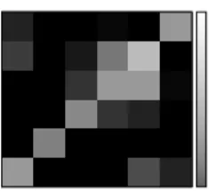
low - high correlation
Figure 1: Label relationships displayed in the form of a heatmap where lighter shades indicate higher probabilities. Prior probabilities are displayed in the diagonal.
Importantly, in multi-label data, relationships exist be-tween the labels. In the absence of label relationships, multi-label data is uninteresting, since this would mean we could simply treat each label a separate binary problem, with-out any loss of information. Aside from generally finding that P(lj|lk) ≈ P(lj), which we expect in the absence of any strong relationship (as implied by Bayes’ rule), we note strong domain-dependent relationships between labels. Fig-ure 1 shows a representation of the relationships between
labels in theScenedataset (mentioned later). The domain
dependent relationships are seen clearly, for example labels 4 and 0.
Additionally to relationships between labels, there also exist relationships between labels and attributes. Clearly, simply more adding labels to a single-label example will not create a realistic multi-label example.
We demonstrate some of these relationships using text data, since it is both intuitive to examine, and also typical to multi-label data streams (although we have discovered similar effects in other kinds of data). Tables 1 and 2 re-late to two text corpora which we worked with in [15]. They
show the most frequent words for labels occurringexclusively
of each other, togetherin combinationwith each other, and
found globally across the dataset. Table 3 shows the
aver-age and standard deviations for specific word-features taken from the tables (in terms of predicting specific labels). In reference to these samples, influences between features and labels can be observed.
An attribute may identify a certain label:xa→lj, where
xa ∈ X and lj ∈ L. An intuitive example is the word
fea-ture ‘linux’ (see Tables 1, and 3) which pertains strongly
to the labelLinux– occurring in over half of all documents
associated with this label.
An attribute may identify acombination of labels;xa→
S, wherexa∈ X andS⊆ L; i.e. several labels co-occurring
together, but not necessarily either of the labels occurring
individually. This is the case in the20 Newsgroups dataset
for the word ‘arms’ (see Tables 2 and 3), which tends to occur frequently only when the newsgroup post is also posted to
both politics.gunsand misc.religion.
There are also variousrandom effectsornon-effects. Words
like ‘anonymous’ inSlashdotare generic and do not strongly
indicate the presence or absence of either labels or combina-tions of labels. Such features are not helpful to classification and should already arguably have been removed by efficient feature selection. Therefore we need not consider them in a synthetic stream. Surprisingly, the case where an attribute value is near the average of the attribute of a combination; i.e. P(xa|{l1, l2})≈(P(xa|l1)+P(xa|l2))/2, isnotcommon.
Table 1:Slashdot. Most frequent words for labelsLinuxand
Mobile
Global Linux Mobile {Linux,Mobile}
anonymous linux mobile linux reader ubuntu iphone open game source anonymous windows story open reader phone reports released phone netbook world anonymous android source years kernel apple mobile released software phones free
Table 2: 20 Newsgroups. Most frequent words for labels
politics.gunsandreligion.misc
Global politics.guns religion.misc {politics.guns,
religion.misc}
don people don jews 1 don people arms 2 gun christian bear people time god don time government years koresh good fbi good fbi make guns time people 3 waco make news
Aside from parameters|L|andz, our framework only
re-quires a single-label binary generatorg. A prime advantage
of our framework is that any single-label stream generator can be used forg. The initialisation process is as follows.
Prior probabilities are generated for all labels, i.e. P(lj)∈ [0.0,1.0] for allj = 1· · · |L|. These probabilities are scaled
according to parameterzso as to approximate to the desired
average number of labels. Following this, a|L| × |L|
proba-bility matrixm (where eachm[j][k] =P(lj|lk)) is filled for
∀m[j][k] : 0< j < k≤ |L|withP(lj|lk)≈P(lj). We over-ride some of these values with random probabilities (within the constraints of probability laws) to simulate the domain-dependent relationships. Thereafter, the remaining half of the matrix ∀m[j][k] : 0 < k < j ≤ |L| can be calculate according to Bayes’ rule:
P(lj|lk) =
P(lk|lj)·P(lj)
P(lk)
Using the resulting matrix we can calculate the top n
most-likely combinationsS1· · ·Sn where eachSi⊆ L. We
usen=|L|2 . These include single-labels, i.e. |Si| ≥1. From
this list we create an attribute-label mapping ζ of size d
where each attribute influences the presence or absence of
a either a single label (|Si| = 1) or combination of labels
(|Si|>1), i.e. ζ[a]→Sa modnfor eachx[a].
Finally, the binary generator is initialised, and the gener-ation process can begin. Figure 2 illustrates the overall pro-cess for generating a multi-label example. An initial label is chosen at random from the distribution of prior probabili-ties. Labels may then be added to this label to form a label set. A multi-label instance space is formed for these labels
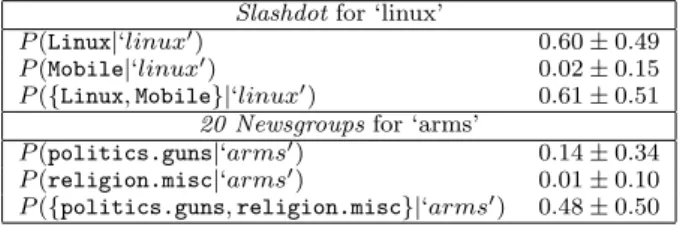
Table 3: Distributions of word frequencies for certain labels both individually and in combination.
Slashdotfor ‘linux’
P(Linux|‘linux0) 0.60±0.49 P(Mobile|‘linux0) 0.02±0.15 P({Linux,Mobile}|‘linux0) 0.61±0.51
20 Newsgroupsfor ‘arms’
P(politics.guns|‘arms0) 0.14±0.34 P(religion.misc|‘arms0) 0.01±0.10
P({politics.guns,religion.misc}|‘arms0) 0.48±0.50
nextInstance()
1 randomly pick an initial label (index) for this example
2 S={l←pick(norm([P(l1),· · ·, P(l|L|)]))}
3 add labels
4 whilel≥0
5 doS←S∪l
6 l←addLabel(S)
7 generate an instance space for these labels
8 x←genML(S)
9 return(x, S)
Figure 2: Algorithm for generating a multi-label example.
genML(S)
1 Create an empty instance
2 xm= (·,·,· · ·,·)d
3 Generate two binary examples (positive; negative)
4 x+1←g.genSL(+1)
5 x−1←g.genSL(−1)
6 Fill the instance spacexmaccording tox−1, x+1 andζ
7 fora←1. . . d 8 do 9 if ζ[a]⊆S 10 thenxm[a]←x+1[a] 11 else xm[a]←x−1[a] 12 returnxm
Figure 3: Generating a multi-label instance to fit a given label set.
according to the feature-label mappingζ. Finally, instance
and label-set are returned together as a newly generated multi-label example.
The auxiliary functionpick(R) simply returnsjwith
prob-abilityR[j], and−1 with probability 1.0−P|R|
j R[j].
Equa-tion 1 defines the funcEqua-tionaddLabel(S) which takes a label
setSand returns a label likely to be added to this set. Note
that Q|S|
k=1P(lj|S[k]) = 0 whenever lj ∈ S (a label
can-not be added twice). A null label is possible, in which case
addLabel(S) =−1 returns and the process of adding labels
must halt. The process of forming a multi-label instance for
a label set usingζ is outlined in Figure 3, and exemplified
in Figure 4.
addLabel(S) : return pick(Qk|S=1| P(l1|S[k]),· · ·, Q|S|
k=1P(lN|S[k])) (1)
3.3
Adding Concept Drift
A new experimental framework for concept drift in stream-ing data was presented in [2]. The main goal of this frame-work is to introduce artificial drift to data stream generators in a straightforward way.
Considering data streams as data generated from pure dis-tributions, we can model a concept drift event as a weighted combination of two pure distributions that characterizes the target concepts before and after the drift. This framework
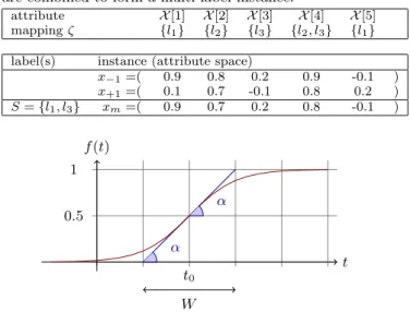
Figure 4: A small illustration of how two binary instances are combined to form a multi-label instance.
attribute X[1] X[2] X[3] X[4] X[5] mappingζ {l1} {l2} {l3} {l2, l3} {l1}
label(s) instance (attribute space)
x−1=( 0.9 0.8 0.2 0.9 -0.1 ) x+1=( 0.1 0.7 -0.1 0.8 0.2 ) S={l1, l3} xm=( 0.9 0.7 0.2 0.8 -0.1 ) t f(t) α α t0 W 0.5 1
Figure 5: A sigmoid functionf(t) = 1/(1 + e−s(t−t0)).
defines the probability that every new instance of the stream belongs to the new concept after the drift. It uses the sig-moid function, as an elegant and practical solution.
We see from Figure 5 that the sigmoid function
f(t) = 1/(1 + e−s(t−t0))
has a derivative at the pointt0 equal tof0(t0) =s/4. The
tangent of angleαis equal to this derivative, tanα=s/4.
We observe that tanα = 1/W, and as s = 4 tanα then
s = 4/W. So the parameter s in the sigmoid gives the
length ofW and the angleα. In this sigmoid model we only
need to specify two parameters :t0 the point of change, and
W the length of change.
Definition 1. Given two data streams a, b, we define
c = a⊕W
t0 b as the data stream built joining the two data
streamsa andb, where t0 is the point of change,W is the length of change and
• Pr[c(t) =a(t)] = e−4(t−t0)/W/(1 + e−4(t−t0)/W)
• Pr[c(t) =b(t)] = 1/(1 + e−4(t−t0)/W).
In order to create a data stream with multiple concept changes, we can build new data streams joining different concept drifts: (((a⊕W0 t0 b)⊕ W1 t1 c)⊕ W2 t2 d). . .
Multi-label concept changes can be formed using the same
method, wherea,b,c, etc. are simply multi-label streams
as defined by our framework.
4.
MULTI-LABEL HOEFFDING TREES
We extend the Hoeffding Tree to deal with multi-label streams since the Hoeffding Tree is the state-of-the-art
clas-sifier for single-label data streams. AMulti-label Hoeffding
Treeis an incremental decision tree classifier for multi-label
data streams that it is based on the use of the Hoeffding bound as a criterion to decide whether to split nodes.
Clare and King [5] adapted C4.5 to multi-label data clas-sification. We use the same strategy to develop a decision tree for multi-label data streams. We present two main ex-tensions: the use of a new definition of entropy to compute information gain, and the use of multi-label classifiers at the leaves.
Information gain is a criterion used in leaf nodes to decide if it is worth splitting them or not. Information gain for
an attributeAin a splitting node is the difference between
the entropy of the training examplesS at the node and the
weighted sum of the entropy of the subsets Sv caused by
partitioning on the valuesvof that attributeA.
Information Gain(S,A) = entropy(S)−X
v∈A
|Sv|
|S|entropy(Sv)
Hoeffding Trees expect that each example belongs to just one class. Entropy is used in C4.5 decision trees and
single-label Hoeffding Trees for a set of examplesSwithN classes
and probabilityp(ci) for each classci in the setS as
entropySL(S) =−
N X
i=1
p(ci) log(p(ci))
To deal with multi-label decision trees, we must use the following definition of entropy:
entropyML(S) = entropySL(S)−
N X
i=1
(1−p(ci)) log(1−p(ci))
Entropy is a measure of the amount of uncertainty in the dataset. For each example, it is the information needed to describe all the classes it belongs to. In the case of multi-label examples, we need to add to the computation of the entropy the information needed to describe all the classes that it doesn’t belong to. We do that by adding the term (1−p(ci)) log(1−p(ci)) for each classci.
The second important extension is the addition of multi-label classification at the leaves. We allow the insertion of any multi-label classifier, and use a majority-label-set classi-fier (the multi-label version of majority-class) as the default classifier.
In [14] we presented the pruned sets methodPS. The
mo-tivation behind PS is to capitalise on the most important
label relationships within a multi-label dataset. PSis based
uponLC, but showed not only an improvement in predictive
performance overLC, but also very significant gains in
effi-ciency. By pruning away infrequently occurring label sets, much unnecessary and detrimental complexity is avoided. A post-pruning step breaks up the pruned sets into more fre-quently occurring subsets, and is able to reintroduce pruned instances into the data, ensuring minimal information loss. Its classification power comes from being able to take into ac-count label combinations directly, and its efficiency makes it
an ideal choice in the data stream problem. LC-based
meth-ods likePSare not naturally suited to data stream settings
on their own because they focus around existing label sets, from which they create class-labels for an underlying
single-label classifier. APS classifier must be completely reset in
order to take into account new combinations (an
incremen-tal version of PSis left for future work). In the leaves of a
the core model structure, and thus becomes a viable
solu-tion.PScan either be primed withninstances and initialised
with these, or reset whenever anADWIN-monitor [1] detects
change to the number of combinations being seen (PSa). PS
requires parameters; we use pruning valuep= 1,
decompo-sition valuen = 1, and Na¨ıve Bayes as a single-label base
classifier in all cases.
5.
EXPERIMENTAL EVALUATION
The data stream evaluation framework and all algorithms evaluated in this paper were implemented in the Java
pro-gramming language extending the MOA software. MOA
includes a collection of offline and online methods as well as tools for evaluation.
5.1
Evaluation Measures and Methodology
Multi-label evaluation is not as straightforward as
single-label evaluation, where the simpleaccuracymetric often
suf-fices. In the single-label context, accuracy is simply the
number of correctly labelled test instances relative to the total number of instances. However, this measure does not transfer well to the extra dimension of the label space in the
multi-label context. If accuracy isexample-based, then the
label set must match exactly for each example to be con-sidered correct, and the measure tends to be overly harsh. Other measures of predictive performance are needed.
We use the notation from Section 3.2, where Yi is the
predictedset for theith example.
We usesubset accuracyas defined in [18]:
SubsetAccuracy = 1 |D| |D| X i=1 |Si∩Yi| |Si∪Yi|
WhereYiis the predicted label set for theith example, which
is compared to Si, the actual set. |D| is the number of
examples that we are evaluating.
As we argued in [16], it is essential to include several eval-uation measures in any multi-label experiment. Given the extra label dimension, it is otherwise possible to optimise for certain evaluation measures. For this reason we include two contrasting measures; macro-averaged F1, and log loss. The F-measure is the harmonic mean between precision and recall, common to information retrieval. It can be calcu-lated from the true positives (tp), true negatives (tn), false
positives (f p) and false negatives (f n). While subset
ac-curacy is averaged over examples, we use a macro-average F-measure; averaged over all labels:
F1M acro(L)= 1 |L| |L| X j=1 F1(tpj, f pj, tnj, f nj) (2)
Finally we uselog loss, which we introduced in [16],
dis-tinct from other measures because it punishes worse errors more harshly, and thus provides a good contrast to other measures. Rather than comparing predicted and actual sets, the prediction confidences of classifiers are evaluated, and the error is graded by the confidence at which it was pre-dicted: predicting false positives with low confidence induces logarithmically less penalty than predicting with high con-fidence. Ifλj is the prediction confidence for thejth label, andlj∈ {0,1}, then: LogLoss = 1 |D| |D| X i=1 |L| X j=1 −max“log 1 |L|, log(λj)lj+ log(1−λj)(1−lj) ”
We have used a dataset-dependent maximum oflog(|L|1 )
to limit the magnitudes of the penalty. Such a limit, as ex-plained in [17], serves to smooth the values and to prevent a small subset of poorly predicted labels from greatly distort-ing the overall error. Note that, as a loss metric, the best possible score for log loss is 0.0.
Many multi-label algorithms, including most ensemble meth-ods, initially result in a ranking, and require an extra process to separate relevant and irrelevant labels for each example to yield multi-label classifications. For log loss evaluation, we do not need to consider such a separation. For subset ac-curacy and F1-measure, we simply adjust a threshold over time according to label cardinality. If the predicted label cardinality becomes lower than the actual label cardinality, the threshold is adjusted upward, and adjusted downward in the case of the reverse. Obviously threshold adjustment is done posterior to each prediction.
In the analysis of running time we measure train time in seconds, and we measure memory use in terms of megabytes. The evaluation methodology used was prequential [8], where every example was used for testing the model before using it to train. Results are averages of 10 runs.
5.2
Datasets
Table 4 provides statistics for a collection of multi-label
datasets. Scene and Yeast are well known datasets in the
multi-label literature (see for example [18]), although they are unfortunately of insufficient size for a data-stream set-ting. Nevertheless, we display them to give an idea of
typ-ical multi-label dimensions. TMC20071 contains instances
of aviation safety reports that document problems which
occurred during certain flights. The labels represent the
problems being described by these reports. We use a re-duced version of this dataset with the top 500 features
se-lected, as specified in [19]. IMDBcomes from the Internet
Movie Database http://imdb.org (we obtained the data
from http://www.imdb.com/interfaces#plain). We used the movie plot text summaries labelled with the relevant
genres.MediaMilloriginates from the 2005 NIST TRECVID
challenge dataset, a competition2 which contains video data
annotated with various concepts. In the final row of the ta-ble we list the range of parameters we used to generate the synthetic data.
Several different schemes are used as base generators for single-label binary synthetic data streams as required by the multi-label generation framework. The Random Tree Gener-ator is the generGener-ator proposed by Domingos and Hulten [6], producing concepts that in theory should favour decision tree learners. It constructs a decision tree by choosing at-tributes at random to split, and assigning a random class label to each leaf. Once the tree is built, new examples are generated by assigning uniformly distributed random val-ues to attributes which then determine the class label via
1
http://www.cs.utk.edu/tmw07/
2http://www.science.uva.nl/research/mediamill/
the tree. The generator has parameters to control the num-ber of classes, attributes, nominal attribute labels, and the depth of the tree. For consistency between experiments, two random trees were generated and fixed as the base concepts
for testing—onesimpleand the othercomplex, where
com-plexity refers to the number of attributes involved and the size of the tree.
The RBF (Radial Basis Function) generator was devised to offer an alternate complex concept type that is not straight-forward to approximate with a decision tree model. This generator effectively creates a normally distributed hyper-sphere of examples surrounding each central point with vary-ing densities. Drift is introduced by movvary-ing the centroids with constant speed initialized by a drift parameter.
We use the following synthetic streams as the base
gener-ators (parameterg) in our multi-label framework:
• rts: Simple random tree that has ten nominal
at-tributes with five values each, and a tree depth of five, with leaves starting at level three and a 0.15 chance of leaves thereafter.
• rtc: Simple random tree that has one hundred
nomi-nal attributes with five values each, a tree depth of five, with leaves starting at level three and a 0.15 chance of leaves thereafter.
• rrbfs refers to a simple random RBF data set—50
centers and 10 attributes.
• rrbfcis more complex—50 centres, 100 attributes.
• Syntis defined as (((RT Sz=1.5⊕Wt0RT Sz=4)⊕ W 2t0RT Sz=2.5)⊕ W 3t0RT Sz=9.5)
For the multi-label generation process, we experiment with
parametersz= 1.5 (approximate average number of labels
per example) and|L|= 8 (number of labels) for streamsrts
andrrbfs, and z = 5.0 and|L|= 30 for streams rtcand
rrbfc.
5.3
Methods
We test the aforementioned data streams with the follow-ing classifiers:
• HT: Multi-label Hoeffding Tree
• HT-PS: Multi-label Hoeffding Tree withPSclasssifier at the leaves, and using the first one thousand examples to compute the label combinations
• HT-PSA: Multi-label Hoeffding Tree withPSclasssifier
at the leaves, and usingADWINmonitoring the number
of label combinations, and computing the label com-binations every time a change is detected.
• BBR: Bagging of tenBRclassifiers with Hoeffding Trees
as the base classifier.
• BAG HT-PSA:ADWINBagging of ten decision trees, using
HT-PSA as base classifier. ADWINmonitors the number
of label combinations.
5.4
Results
The prequential evaluation procedure was carried out on one million examples from the RandomTree and Random-RBF datasets. Tables 5, 6 and 7 display the final subset ac-curacy, log-loss, and F-1-Macro measures respectively. Ta-ble 7 shows the culmative train time of the methods, and
Table 8 the memory used. Additionally, the prequential
learning curves with a window size of 10,000 for synthetic
data, and 10% for real datasets, were plotted for for subset
accuracy, log loss, and macro F1-Measure forSynton one
million samples dataset are plotted in Figures 6, 7, and 8.
Accuracy 20 30 40 50 60 70 80 10.000 140.000 270.000 400.000 530.000 660.000 790.000 920.000 Instances A c c u ra c y ( % ) BAG HT-PSA HT-PSA HT-PS HT BBR
Figure 6: Subset accuracy on Synt with three concept
drifts. Log-Loss 2 2,5 3 3,5 4 4,5 5 10.000 140.000 270.000 400.000 530.000 660.000 790.000 920.000 Instances L o g -L o s
s BAG HT-PSAHT-PSA
HT-PS HT BBR
Figure 7: Log-loss onSyntwith three concept drifts.
5.5
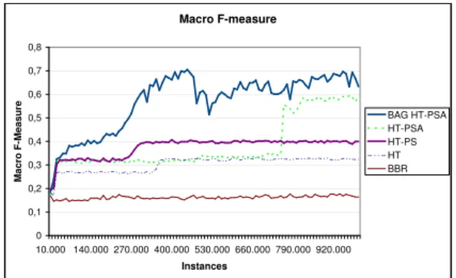
Discussion
HT-PSand HT-PSAperformed well in different situations.
As evident from Tables 5 and 7, HT-PSA is the stronger
method for adapting to concept drift because of the ADWIN
change-monitor.
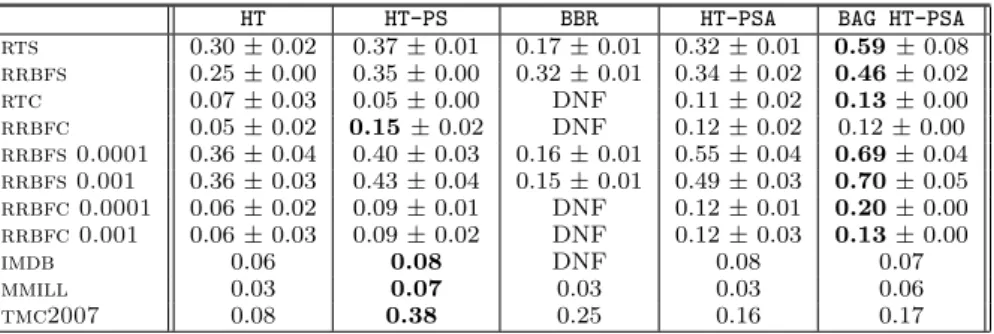
BAG HT-PSAperforms the best overall, particularly under log loss. Strong performance was expected from a bagging
HT HT-PS BBR HT-PSA BAG HT-PSA rts 0.52±0.01 0.54±0.00 0.24±0.01 0.42±0.01 0.60±0.07 rrbfs 0.33±0.00 0.42±0.00 0.48±0.01 0.34±0.01 0.49±0.03 rtc 0.16±0.03 0.08±0.01 DNF 0.12±0.03 0.12±0.00 rrbfc 0.16±0.02 0.15±0.02 DNF 0.14±0.03 0.08±0.00 rrbfs 0.0001 0.50±0.05 0.51±0.05 0.22±0.01 0.58±0.04 0.69±0.03 rrbfs 0.001 0.55±0.04 0.56±0.05 0.22±0.00 0.58±0.04 0.69±0.04 rrbfc 0.0001 0.15±0.01 0.14±0.01 DNF 0.14±0.02 0.20±0.00 rrbfc 0.001 0.15±0.03 0.14±0.03 DNF 0.13±0.03 0.10±0.00 imdb 0.20 0.10 DNF 0.15 0.15 mmill 0.31 0.23 0.16 0.05 0.21 tmc2007 0.17 0.43 0.39 0.26 0.24
Table 5: Comparison of methods. Subset accuracy is measured over the one million prequential evaluation. The best individual
accuracies are indicated in boldface.
HT HT-PS BBR HT-PSA BAG HT-PSA
rts 2.61±0.04 2.72±0.02 3.12±0.00 3.89±0.08 2.32±0.18 rrbfs 3.53±0.02 3.37±0.02 2.57±0.01 3.92±0.12 2.61±0.10 rtc 14.59±0.70 16.24±0.59 DNF 14.74±0.57 8.41±0.00 rrbfc 14.10±0.40 13.39±0.26 DNF 13.65±0.45 8.00±0.00 rrbfs 0.0001 2.81±0.30 2.91±0.31 3.15±0.00 2.48±0.26 1.96±0.07 rrbfs 0.001 2.47±0.25 2.66±0.28 3.14±0.00 2.52±0.26 1.95±0.11 rrbfc 0.0001 14.27±0.36 14.77±0.24 DNF 13.64±0.23 7.64±0.00 rrbfc 0.001 14.84±0.61 14.73±0.62 DNF 13.85±0.51 8.02±0.00 imdb 7.62 10.33 NF 10.39 6.08 mmill 19.61 25.22 14.18 20.45 13.52 tmc2007 7.89 6.41 4.90 8.09 5.14
Table 6: Comparison of methods. LogLoss is measured as the final average over one million examples using prequential evaluation. The
best individual accuracies are indicated in boldface.
Macro F-measure 0 0,1 0,2 0,3 0,4 0,5 0,6 0,7 0,8 10.000140.000 270.000 400.000 530.000 660.000 790.000 920.000 Instances M a c ro F -M e a s u re BAG HT-PSA HT-PSA HT-PS HT BBR
Figure 8: Macro F1-measure onSynt with three concept
drifts.
scheme, since ensembles are well known for increasing the performance of base models.
BBR ran into time and memory complexity issues. As a
separate Hoeffding tree is needed for each single label in
each bag. Surprisingly,BBRis not at all competitive overall,
although is competitive in log loss in some situations, likely due to conservative prediction.
6.
CONCLUSIONS AND FUTURE WORK
Table 4: A sample of multi-label datasets.
|D| |L| |X | avg(|S|) Scene 2407 6 294n 1.07 Yeast 2417 14 103n 4.24 TMC2007 28596 22 500b 2.16 MediaMill 43907 101 120n 4.38 IMDB 95424 28 1001b 1.92 Synthetic 1E6 {8,30} {30,100} {1.5,5.0}
nindicates numeric attributes, andbboolean.
We have presented an experimental framework for multi-label data stream classification, to help performing new ex-perimental multi-label data stream benchmarks. The new methods we presented combine state-of-the-art approaches in both data stream and label classification:
multi-label Hoeffding trees with PS classifiers at the leaves, and
additionally in anADWIN-bagging ensemble framework.
We carried out an in depth experimental evaluation on both real and synthetic datasets using three multi-label eval-uation measures, as well as measuring time and memory. We obtain satisfying results for the single multi-label Hoeffding tree, both in terms of runtime and memory consumption, and even better results under a bagging scheme which is able to adapt to concept drift.
As future work, we would like to build new incrementalPS
methods, and experiment with multi-label ensemble meth-ods based on boosting.
7.
REFERENCES
HT HT-PS BBR HT-PSA BAG HT-PSA rts 0.30±0.02 0.37±0.01 0.17±0.01 0.32±0.01 0.59±0.08 rrbfs 0.25±0.00 0.35±0.00 0.32±0.01 0.34±0.02 0.46±0.02 rtc 0.07±0.03 0.05±0.00 DNF 0.11±0.02 0.13±0.00 rrbfc 0.05±0.02 0.15±0.02 DNF 0.12±0.02 0.12±0.00 rrbfs 0.0001 0.36±0.04 0.40±0.03 0.16±0.01 0.55±0.04 0.69±0.04 rrbfs 0.001 0.36±0.03 0.43±0.04 0.15±0.01 0.49±0.03 0.70±0.05 rrbfc 0.0001 0.06±0.02 0.09±0.01 DNF 0.12±0.01 0.20±0.00 rrbfc 0.001 0.06±0.03 0.09±0.02 DNF 0.12±0.03 0.13±0.00 imdb 0.06 0.08 DNF 0.08 0.07 mmill 0.03 0.07 0.03 0.03 0.06 tmc2007 0.08 0.38 0.25 0.16 0.17
Table 7: Comparison of methods. Macro F1-Measure is measured as the final average over one million examples using prequential
evaluation. The best individual accuracies are indicated in boldface.
HT HT-PS BBR HT-PSA BAG HT-PSA
rts 4.51 31.78 106.37 21.37 227.01 rrbfs 0.96 29.20 48.71 6.19 81.27 rtc 36.20 30.92 DNF 36.15 533.10 rrbfc 9.46 32.14 DNF 19.13 237.32 rrbfs 0.0001 1.20 31.25 48.19 6.87 86.60 rrbfs 0.001 1.19 31.63 49.30 7.07 85.10 rrbfc 0.0001 11.79 31.22 DNF 19.87 187.32 rrbfc 0.001 12.20 31.73 DNF 21.43 179.09 imdb 23.38 142.59 DNF 24.64 179.65 mmill 7.99 10.94 260.88 2.37 19.69 tmc2007 1.54 5.33 237.83 1.44 13.28
Table 8: Comparison of methods. Memory in megabytes.
HT HT-PS BBR HT-PSA BAG HTPSA
rts 1.24 13.97 133.55 5.12 40.73 rrbfs 35.07 239.73 209.08 56.39 244.76 rtc 9.23 745.94 DNF 115.84 1134.59 rrbfc 324.75 1758.66 DNF 537.22 4693.80 rrbfs 0.0001 258.71 360.19 96.61 359.41 4123.85 rrbfs 0.001 8.30 48.52 204.46 19.76 213.31 rrbfc 0.0001 9.08 965.32 DNF 125.16 1291.70 rrbfc 0.001 273.99 1228.54 DNF 472.93 5093.07 imdb 263.59 2070.93 DNF 410.15 4927.07 mmill 139.43 302.65 2552.27 226.90 2989.63 tmc2007 64.56 194.41 1176.92 86.27 829.46
Table 9: Comparison of methods. Time in seconds.
closed unlabeled rooted trees in data streams. InKDD
’08, 2008.
[2] A. Bifet, G. Holmes, B. Pfahringer, R. Kirkby, and
R. Gavald`a. New ensemble methods for evolving data
streams. InKDD ’09. ACM, 2009.
[3] L. Cai.Multilabel Classification over Category
Taxonomies. PhD thesis, Department of Computer Science, Brown University, May 2008.
[4] W. Cheng and E. H¨ullermeier. Combining
instance-based learning and logistic regression for
multilabel classification.Machine Learning,
76(2-3):211–225, 2009.
[5] A. Clare and R. D. King. Knowledge discovery in
multi-label phenotype data. InPKDD ’01, pages
42–53, 2001.
[6] P. Domingos and G. Hulten. Mining high-speed data
streams. InKDD ’00, pages 71–80, 2000.
[7] J. F¨urnkranz, E. H¨ullermeier, E. Loza Menc´ıa, and K. Brinker. Multilabel classification via calibrated
label ranking.Machine Learning, 73(2):133–153,
November 2008.
[8] J. Gama, R. Sebasti˜ao, and P. P. Rodrigues. Issues in
evaluation of stream learning algorithms. InKDD ’09,
pages 329–338, 2009.
[9] S. Godbole and S. Sarawagi. Discriminative methods
for multi-labeled classification. InPAKDD ’04, pages
22–30. Springer, 2004.
[10] G. Holmes, R. Kirkby, and B. Pfahringer. MOA: Massive Online Analysis.
http://www.cs.waikato.ac.nz/ abifet/moa/. 2007. [11] N. Oza and S. Russell. Online bagging and boosting.
InArtificial Intelligence and Statistics 2001, pages 105–112. Morgan Kaufmann, 2001.
[12] S.-H. Park and J. F¨urnkranz. Multi-label classification
with label constraints. Technical report, Knowledge Engineering Group, TU Darmstadt, 2008.
[13] W. Qu, Y. Zhang, J. Zhu, and Q. Qiu. Mining multi-label concept-drifting data streams using
dynamic classifier ensemble. InACML, 2009.
[14] J. Read, B. Pfahringer, and G. Holmes. Multi-label classification using ensembles of pruned sets. In
ICDM’08, pages 995–1000. IEEE, 2008.
[15] J. Read, B. Pfahringer, and G. Holmes. Generating
synthetic multi-label data streams. InMLD ’09,
September 2009.
[16] J. Read, B. Pfahringer, G. Holmes, and E. Frank. Classifier chains for multi-label classification. In
ECML ’09, pages 254–269. Springer-Verlag, 2009. [17] R. E. Schapire and Y. Singer. Improved boosting
algorithms using confidence-rated predictions.
Machine Learning, 37(3):297–336, December 1999. [18] G. Tsoumakas and I. Katakis. Multi label
classification: An overview.International Journal of
Data Warehousing and Mining, 3(3), 2007.
[19] G. Tsoumakas and I. P. Vlahavas. Random k-labelsets: An ensemble method for multilabel classification. In
ECML ’07, pages 406–417. Springer-Verlag, 2007. [20] R. Yan, J. Tesic, and J. R. Smith. Model-shared
subspace boosting for multi-label classification. In
KDD ’07, pages 834–843. ACM, 2007.
[21] M.-L. Zhang and Z.-H. Zhou. Ml-knn: A lazy learning
approach to multi-label learning.Pattern Recogn.,