Edinburgh Research Explorer
Random-projection ensemble classification
Citation for published version:
Cannings, T & Samworth, RJ 2017, 'Random-projection ensemble classification' Journal of the Royal
Statistical Society: Series B, vol. 79, no. 4, pp. 959-1035. DOI: 10.1111/rssb.12228
Digital Object Identifier (DOI):
10.1111/rssb.12228
Link:
Link to publication record in Edinburgh Research Explorer
Document Version:
Publisher's PDF, also known as Version of record
Published In:
Journal of the Royal Statistical Society: Series B
General rights
Copyright for the publications made accessible via the Edinburgh Research Explorer is retained by the author(s)
and / or other copyright owners and it is a condition of accessing these publications that users recognise and
abide by the legal requirements associated with these rights.
Take down policy
The University of Edinburgh has made every reasonable effort to ensure that Edinburgh Research Explorer
content complies with UK legislation. If you believe that the public display of this file breaches copyright please
contact [email protected] providing details, and we will remove access to the work immediately and
investigate your claim.
©2017 The Authors Journal of the Royal Statistical Society: Series B
(Statistical Methodology) published by John Wiley & Sons Ltd on behalf of Royal Statistical Society.
This is an open access article under the terms of the Creative Commons Attribution License, which permits use, dis-tribution and reproduction in any medium, provided the original work is properly cited.
1369–7412/17/79959 79,Part4,pp.959–1035
Random-projection ensemble classification
Timothy I. Cannings and Richard J. SamworthUniversity of Cambridge, UK
[Read before The Royal Statistical Society at a meeting organized by the Research Sec-tionon Wednesday, March 15th, 2017, Professor C. Lengin the Chair]
Summary.We introduce a very general method for high dimensional classification, based on careful combination of the results of applying an arbitrary base classifier to random projections of the feature vectors into a lower dimensional space. In one special case that we study in detail, the random projections are divided into disjoint groups, and within each group we select the projection yielding the smallest estimate of the test error. Our random-projection ensemble classifier then aggregates the results of applying the base classifier on the selected projections, with a data-driven voting threshold to determine the final assignment. Our theoretical results elucidate the effect on performance of increasing the number of projections. Moreover, under a boundary condition that is implied by the sufficient dimension reduction assumption, we show that the test excess risk of the random-projection ensemble classifier can be controlled by terms that do not depend on the original data dimension and a term that becomes negligible as the number of projections increases. The classifier is also compared empirically with several other popular high dimensional classifiers via an extensive simulation study, which reveals its excellent finite sample performance.
Keywords: Aggregation; Classification; High dimensional classification; Random projection
1. Introduction
Supervised classification concerns the task of assigning an object (or a number of objects) to one of two or more groups, on the basis of a sample of labelled training data. The problem was first studied in generality in the famous work of Fisher (1936), where he introduced some of the ideas of linear discriminant analysis (LDA) and applied them to his iris data set. Nowa-days, classification problems arise in a plethora of applications, including spam filtering, fraud detection, medical diagnoses, market research, natural language processing and many others.
In fact, LDA is still widely used today and underpins many other modern classifiers; see,
for example, Friedman (1989) and Tibshiraniet al. (2002). Alternative techniques include
sup-port vector machines (SVMs) (Cortes and Vapnik, 1995), tree classifiers and random forests
(RFs) (Breimanet al., 1984; Breiman, 2001), kernel methods (Hall and Kang, 2005) and nearest
neighbour classifiers (Fix and Hodges, 1951). More substantial overviews and detailed
discus-sion of these techniques, and others, can be found in Devroyeet al.(1996) and Hastieet al.
(2009).
An increasing number of modern classification problems arehigh dimensional, in the sense
that the dimensionpof the feature vectors may be comparable with or even greater than the
number of training data points,n. In such settings, classical methods such as those mentioned
in the previous paragraph tend to perform poorly (Bickel and Levina, 2004) and may even be
Address for correspondence: Richard J. Samworth, Statistical Laboratory, Centre for Mathematical Sciences, University of Cambridge, Wilberforce Road, Cambridge, CB3 0WB, UK.
intractable; for example, this is so for LDA, where the problems are caused by the fact that the
sample covariance matrix is not invertible whenpn.
Many methods proposed to overcome such problems assume that the optimal decision
bound-ary between the classes is linear, e.g. Friedman (1989) and Hastieet al. (1995). Another common
approach assumes that only a small subset of features are relevant for classification. Examples of works that impose such a sparsity condition include Fan and Fan (2008), where it was also
assumed that the features are independent, as well as Tibshiraniet al. (2003), where soft
thresh-olding was used to obtain a sparse boundary. More recently, Witten and Tibshirani (2011) and Fanet al.(2012) both solved an optimization problem similar to Fisher’s linear discriminant,
with the addition of anl1penalty term to encourage sparsity.
In this paper we attempt to avoid the curse of dimensionality by projecting the feature vectors at random into a lower dimensional space. The use of random projections in high dimensional statistical problems is motivated by the celebrated Johnson–Lindenstrauss lemma (e.g. Dasgupta
and Gupta (2002)). This lemma states that, givenx1,: : :,xn∈Rp,∈.0, 1/andd >8 log.n/=2,
there is a linear mapf:Rp→Rdsuch that
.1−/xi−xj2f.xi/−f.xj/2.1+/xi−xj2,
for alli,j=1,: : :,n. In fact, the functionf that nearly preserves the pairwise distances can be
found in randomized polynomial time by using random projections distributed according to Haar measure, as described in Section 3 below. It is interesting to note that the lower bound
ondin the Johnson–Lindenstrauss lemma does not depend onp; this lower bound is optimal
up to constant factors (Larsen and Nelson, 2016). As a result, random projections have been
used successfully as a computational time saver: whenpis large compared with log.n/, we may
project the data at random into a lower dimensional space and run the statistical procedure on the projected data, potentially making great computational savings, while achieving comparable or even improved statistical performance. As one example of the above strategy, Durrant and Kab´an (2013) obtained Vapnik–Chervonenkis-type bounds on the generalization error of a linear classifier trained on a single random projection of the data. See also Dasgupta (1999),
Ailon and Chazelle (2006) and McWilliamset al. (2014) for other instances.
Other works have sought to reap the benefits of aggregating over many random projections.
For instance, Marzettaet al.(2011) considered estimating ap×ppopulation inverse covariance
(precision) matrix by usingB−1ΣBb=1ATb.AbΣˆATb/−1Ab, where ˆΣdenotes the sample covariance
matrix andA1,: : :,ABare random projections fromRptoRd. Lopeset al.(2011) used this
esti-mate when testing for a difference between two Gaussian population means in high dimensions, whereas Durrant and Kab´an (2015) applied the same technique in Fisher’s linear discriminant for a high dimensional classification problem.
Our proposed methodology for high dimensional classification has some similarities to the techniques described above, in the sense that we consider many random projections of the
data, but is also closely related tobagging (Breiman, 1996), since the ultimate assignment of
each test point is made by aggregation and a vote. Bagging has proved to be an effective tool for improving unstable classifiers. Indeed, a bagged version of the (generally inconsistent) 1-nearest-neighbour classifier is universally consistent as long as the resample size is carefully chosen: see Hall and Samworth (2005); for a general theoretical analysis of majority voting approaches, see also Lopes (2016). Bagging has also been shown to be particularly effective in high dimensional problems such as variable selection (Meinshausen and B ¨uhlmann, 2010; Shah and Samworth, 2013). Another related approach to ours is Blaser and Fryzlewicz (2015), who considered ensembles of random rotations, as opposed to projections.
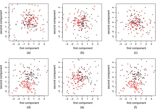
−3 −2 −1 −3 −2 −1 first component second component −3 −2 −1 −3 −2 −1 first component second component −3 −2 −1 −3 −2 −1 first component second component −3 −2 −1 −3 −2 −1 3 first component second component −3 −2 −1 −3 −2 −1 3 first component second component −3 −2 −1 0 1 2 3 0 1 2 3 0 1 2 3 0 1 2 3 0 1 2 3 0 1 2 3 −3 −2 −1 0123 0123 0123 012 012 0123 first component second component (a) (b) (c) (d) (e) (f)
Fig. 1. Different two-dimensional projections of 200 observations inpD50 dimensions: (a)–(c) three pro-jections drawn from Haar measure; (d)–(f) the projected data after applying the propro-jections with smallest estimate of test error out of 100 Haar projections with (d) LDA, (e) quadratic discriminant analysis and (f) k-nearest neighbours
One of the basic but fundamental observations that underpins our proposal is the fact that aggregating the classifications of all random projections is not always sensible, since many of these projections will typically destroy the class structure in the data; see Figs 1(a)–1(c). For this reason, we advocate partitioning the projections into disjoint groups, and within each group we retain only the projection yielding the smallest estimate of the test error. The attraction of this strategy is illustrated in Figs 1(d)–1(f), where we see a much clearer partition of the classes. Another key feature of our proposal is the realization that a simple majority vote of the classifications based on the retained projections can be highly suboptimal; instead, we argue that the voting threshold should be chosen in a data-driven fashion in an attempt to minimize the test error of the infinite simulation version of our random-projection ensemble classifier. In fact, this estimate of the optimal threshold turns out to be remarkably effective in practice; see Section 5.2 for further details. We emphasize that our methodology can be used in conjunction with any base classifier, though we particularly have in mind classifiers designed for use in low dimensional settings. The random-projection ensemble classifier can therefore be regarded as a general technique for either extending the applicability of an existing classifier to high dimensions, or improving its performance. The methodology is implemented in an R package RPEnsemble(Cannings and Samworth, 2016).
Our theoretical results are divided into three parts. In the first, we consider a generic base
classifier and a generic method for generating the random projections intoRd and quantify
the difference between the test error of the random-projection ensemble classifier and its infin-ite simulation counterpart as the number of projections increases. We then consider selecting
random projections from non-overlapping groups by initially drawing them according to Haar measure, and then within each group retaining the projection that minimizes an estimate of the test error. Under a condition that is implied by the widely used sufficient dimension reduction
assumption (Li, 1991; Cook, 1998; Leeet al., 2013), we can then control the difference between
the test error of the random-projection classifier and the Bayes risk as a function of terms that depend on the performance of the base classifier based on projected data and our method for estimating the test error, as well as a term that becomes negligible as the number of projections increases. The final part of our theory gives risk bounds for the first two of these terms for
spe-cific choices of base classifier, namely Fisher’s linear discriminant and thek-nearest-neighbour
classifier. The key point here is that these bounds depend ondonly, the sample sizenand the
number of projections, and not on the original data dimensionp.
The remainder of the paper is organized as follows. Our methodology and general theory are developed in Sections 2 and 3. Specific choices of base classifier as well as a general sample splitting strategy are discussed in Section 4, whereas Section 5 is devoted to a consideration of the practical issues of computational complexity, choice of voting threshold, projected di-mension and the number of projections used. In Section 6 we present results from an extensive empirical analysis on both simulated and real data where we compare the performance of the random-projection ensemble classifier with several popular techniques for high dimensional classification. The outcomes are very encouraging, and suggest that the random-projection ensemble classifier has excellent finite sample performance in a variety of high dimensional classification settings. We conclude with a discussion of various extensions and open problems. Proofs are given in Appendix A and the on-line supplementary material.
The program code that was used to perform the simulations can be obtained from http://wileyonlinelibrary.com/journal/rss-datasets
Finally in this section, we introduce the following general notation that is used throughout
the paper. For a sufficiently smooth real-valued functiongdefined on a neighbourhood oft∈R,
letg˙.t/andg¨.t/denote its first and second derivatives att, and lettand [[t]] :=t− tdenote
the integer and fractional part oftrespectively.
2. A generic random-projection ensemble classifier
We start by describing our setting and defining the relevant notation. Suppose that the pair.X,Y/
takes values inRp×{0, 1}, with joint distributionP, characterized byπ1:=P.Y=1/, andPr, the
conditional distribution ofX|Y=r, forr=0, 1. For convenience, we letπ0:=P.Y=0/=1−π1.
In the alternative characterization ofP, we letPXdenote the marginal distribution ofXand
writeη.x/:=P.Y=1|X=x/for the regression function. Recall that aclassifieronRpis a Borel
measurable functionC:Rp→{0, 1}, with the interpretation that we assign a pointx∈Rpto
classC.x/. We letCpdenote the set of all such classifiers.
The test error of a classifierCis
R.C/:=
Rp×{0,1}1{C.x/=y}dP.x,y/
and is minimized by theBayesclassifier
CBayes.x/:=
1 ifη.x/12,
0 otherwise
P{C.X/=Y}to make it clear that, whenCis random (depending on training data or random
projections), it should be conditioned on when computingR.C/.) The Bayes risk isR.CBayes/=
E[min{η.X/, 1−η.X/}].
Of course, we cannot use the Bayes classifier in practice, sinceη is unknown. Nevertheless,
we often have access to a sample of training data that we can use to construct an approximation to the Bayes classifier. Throughout this section and Section 3, it is convenient to consider the
training sampleTn:={.x1,y1/,: : :,.xn,yn/}to be fixed points inRp×{0, 1}. Our methodology
will be applied to a base classifierCn=Cn,Tn,d, which we assume can be constructed from an
arbitrary training sampleTn,d of sizeninRd×{0, 1}; thusCnis a measurable function from
.Rd×{0, 1}/ntoCd.
Now assume thatdp. We say that a matrixA∈Rd×p is aprojection ifAAT=Id×d, the
d-dimensional identity matrix. LetA=Ad×p:={A∈Rd×p:AAT=Id×d}be the set of all such
matrices. Given a projectionA∈A, define projected datazAi :=AxiandyAi :=yifori=1,: : :,n,
and letTA
n :={.zA1,yA1/,: : :,.zAn,yAn/}. The projected data base classifier corresponding toCnis
CnA:.Rd×{0, 1}/n→Cp, given by
CAn.x/=CAn,TA
n .x/:=Cn,TnA.Ax/:
Note that althoughCnAis a classifier onRp, the value ofCnA.x/only depends onxthrough its
d-dimensional projectionAx.
We now define a generic ensemble classifier based on random projections. ForB1∈N, let
A1,: : :,AB1 denote independent and identically distributed projections inAd×p, independent
of.X,Y/. The distribution onAis left unspecified at this stage, and in fact our proposed method
ultimately involves choosing this distribution depending onTn.
Now set νn.x/=ν.B1/ n .x/:= 1 B1 B1 b1=1 1 {C Ab 1 n .x/=1} : .1/
Forα∈.0, 1/, therandom-projection ensembleclassifier is defined to be
CRPn .x/:=
1 ifνn.x/α,
0 otherwise. .2/
We emphasize again here the additional flexibility that is afforded by not prespecifying the voting
thresholdαto be12. Our analysis of the random-projection ensemble classifier will require some
further definitions. Let
μn.x/:=E{νn.x/}=P{CA1
n .x/=1}:
(To distinguish between different sources of randomness, we shall writePandEfor the
proba-bility and expectation respectively, taken over the randomness from the projectionsA1,: : :,AB1.
If the training data are random, then we condition onTnwhen computingPandE.) Forr=0, 1,
define distribution functionsGn,r: [0, 1]→[0, 1] byGn,r.t/:=Pr[{x∈Rp:μn.x/t}]. SinceGn,r
is non-decreasing it is differentiable almost everywhere; in fact, however, the following assump-tion will be convenient.
Assumption 1. Gn,0andGn,1are twice differentiable atα.
The first derivatives ofGn,0andGn,1, when they exist, are denoted asgn,0andgn,1respectively;
under assumption 1, these derivatives are well defined in a neighbourhood ofα. Our first main
random-projection ensemble classifier as the number of projections increases. In particular, we show that this expected test error can be well approximated by the test error of the infinite simulation random-projection classifier
CnRPÆ.x/:=
1 ifμn.x/α,
0 otherwise.
Provided thatGn,0andGn,1are continuous atα, we have
R.CnRPÆ/=π1Gn,1.α/+π0{1−Gn,0.α/}: .3/
Theorem 1. Assume assumption 1. Then
E{R.CRPn /}−R.CnRPÆ/=γn.α/ B1 +o 1 B1 asB1→ ∞, where γn.α/:=.1−α−[[B1α]]/{π1gn,1.α/−π0gn,0.α/}+ α.1−α/ 2 {π1g˙n,1.α/−π0g˙n,0.α/}: The proof of theorem 1 in Appendix A is lengthy and involves a one-term Edgeworth ap-proximation to the distribution function of a standardized binomial random variable. One of the technical challenges is to show that the error in this approximation holds uniformly in the
bino-mial proportion. Related techniques can also be used to show thatvar{R.CRPn /}=O.B−11/
un-der assumption 1; see proposition 1 in the on-line supplementary material. Very recently, Lopes (2016) has obtained similar results to this and to theorem 1 in the context of majority vote clas-sification, with stronger assumptions on the relevant distributions and on the form of the voting
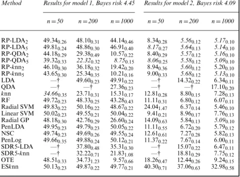
scheme. In Fig. 2, we plot the average error (±2 standard deviations) of the random-projection
ensemble classifier in one numerical example, as we vary B1∈{2,: : :, 500}; this reveals that
the Monte Carlo error stabilizes rapidly, in agreement with what Lopes (2016) observed for a random-forest classifier.
Our next result controls the test excess risk, i.e. the difference between the expected test error and the Bayes risk, of the random-projection classifier in terms of the expected test excess risk of the classifier based on a single random projection. An attractive feature of this result
is its generality: no assumptions are placed on the configuration of the training dataTn, the
distributionP of the test point.X,Y/or on the distribution of the individual projections.
Theorem 2. For eachB1∈N∪{∞}, we have
E{R.CRPn /}−R.CBayes/ 1
min.α, 1−α/[E{R.C
A1
n /}−R.CBayes/]: .4/
WhenB1= ∞, we interpretR.CRPn /in theorem 2 asR.CnRPÆ/. In fact, whenB1= ∞andGn,0
andGn,1are continuous, the bound in theorem 2 can be improved if we are using an ‘oracle’
choice of the voting thresholdα, namely
αÅ∈arg min α∈[0,1] R.C RPÆ n,α/=arg min α∈[0,1] [π1Gn,1.α/+π0{1−Gn,0.α/}], .5/
where we writeCRPn,αÆ to emphasize the dependence on the voting thresholdα. In this case, by
definition ofαÅand then applying theorem 2,
R.CRPn,αÆÆ/−R.CBayes/R.CRP Æ
0 100 200 300 400 500 12 14 16 18 B1 (a) (c) (b) Error 0 100 200 300 400 500 B1 Error 0 100 200 300 400 500 68 1 0 8 1 01 21 41 61 8 8 1 01 21 41 61 8 B1 Error
Fig. 2. Average error ( ) ˙2 standard deviations ( ) over 20 sets of B1B2 projections for
B12{2,. . . , 500}: we use (a) the LDA, (b) quadratic discriminant analysis and (c)k-nearest-neighbour base
classifiers (the plots show the test error for one training data set from model 2; the other parameters are nD50,pD100,dD5 andB2D50)
which improves the bound in expression (4) since 21=min{αÅ,.1−αÅ/}. It is also worth
mentioning that if assumption 1 holds atαÅ∈.0, 1/, andGn,0 andGn,1are continuous, then
π1gn,1.αÅ/=π0gn,0.αÅ/and the constant in theorem 1 simplifies to
γn.αÅ/=αÅ.1−αÅ/
2 {π1g˙n,1.αÅ/−π0g˙n,0.αÅ/}0:
3. Choosing good random projections
In this section, we study a special case of the generic random-projection ensemble classifier that was introduced in Section 2, where we propose a screening method for choosing the random
values in the set{0, 1=n,: : :, 1}. Examples of such estimators include the training error and
leave-one-out estimator; we discuss these choices in greater detail in Section 4. ForB1,B2∈N,
let{Ab1,b2:b1=1,: : :,B1,b2=1,: : :,B2}denote independent projections, independent of.X,Y/,
distributed according to Haar measure onA. One way to simulate from Haar measure on the
setAis first to generate a matrixQ∈Rd×p, where each entry is drawn independently from a
standard normal distribution, and then to takeATto be the matrix of left singular vectors in
the singular value decomposition ofQT(see, for example, Chikuse (2003), theorem 1.5.4). For
b1=1,: : :,B1, let
bÅ2.b1/:= sarg min
b2∈{1,:::,B2}
RAb1,b2
n , .7/
where sargmin denotes the smallest index where the minimum is attained in the case of a tie. We now setAb1:=Ab1,bÆ
2.b1/, and consider the random-projection ensemble classifier from Section
2 constructed by using the independent projectionsA1,: : :,AB1.
Let
RÅn:=min A∈AR
A n
denote the optimal test error estimate over all projections. The minimum is attained here, since
RAn takes only finitely many values. We make the following assumption.
Assumption 2. There existsβ∈.0, 1] such that
P.RAn1,1RÅn+ |n|/β,
wheren=.B2/
n :=E{R.CnA1/−RAn1}.
The quantityn, which depends onB2becauseA1is selected fromB2independent random
projections, can be interpreted as a measure of overfitting. Assumption 2 asks that there is
a positive probability thatRAn1,1 is within|n|of its minimum valueRÅn. The intuition here is
that spending more computational time choosing a projection by increasingB2is potentially
futile: one may find a projection with a lower error estimate, but the chosen projection will not necessarily result in a classifier with a lower test error. Under this condition, the following result controls the test excess risk of our random-projection ensemble classifier in terms of the test
excess risk of a classifier based ond-dimensional data, as well as a term that reflects our ability
to estimate the test error of classifiers on the basis of projected data and a term that depends on the number of projections.
Theorem 3. Assume assumption 2. Then, for eachB1,B2∈N, and everyA∈A,
E{R.CRPn /}−R.CBayes/R.C A n/−R.CBayes/ min.α, 1−α/ + 2|n| −A n min.α, 1−α/+ .1−β/B2 min.α, 1−α/, .8/ whereAn :=R.CAn/−RAn.
Regarding the bound in theorem 3 as a sum of three terms, we see that the final term can be seen as the price that we must pay for the fact that we do not have access to an infinite sample of
random projections. This term can be made negligible by choosingB2to be sufficiently large,
though the value ofB2that is required to ensure that it is below a prescribed level may depend
on the training data. It should also be noted thatn in the second term may increase withB2,
which reflects the fact mentioned previously that this quantity is a measure of overfitting. The behaviour of the first two terms depends on the choice of base classifier, and our aim is to show
that, under certain conditions, these terms can be bounded (in expectation over the training
data) by expressions that do not depend onp.
For this, define the regression function onRdinduced by the projectionA∈Ato beηA.z/:=
P.Y=1|AX=z/. The corresponding induced Bayes classifier, which is the optimal classifier
knowing only the distribution of.AX,Y/, is given by
CA−Bayes.z/:=
1 ifηA.z/1
2,
0 otherwise.
To give a condition under which there is a projectionA∈Afor whichR.CAn/is close to the Bayes
risk, we shall invoke an additional assumption on the form of the Bayes classifier. Assumption 3. There is a projectionAÅ∈Asuch that
PX.{x∈Rp:η.x/12}{x∈Rp:ηA Æ
.AÅx/12}/=0,
whereBC:=.B∩Cc/∪.Bc∩C/denotes the symmetric difference of two setsBandC.
Assumption 3 requires that the set of pointsx∈Rpthat are assigned by the Bayes classifier to
class 1 can be expressed as a function of ad-dimensional projection ofx. If the Bayes decision
boundary is a hyperplane, then assumption 3 holds withd=1. Moreover, proposition 1 below
shows that, in fact, assumption 3 holds under the sufficient dimension reduction condition,
which states thatY is conditionally independent ofXgiven AÅX; see Cook (1998) for many
statistical settings where such an assumption is natural.
Proposition 1. IfYis conditionally independent ofXgivenAÅX, then assumption 3 holds. The following result confirms that under assumption 3, and for a sensible choice of base
classifier, we can hope forR.CnAÆ/to be close to the Bayes risk.
Proposition 2. Assume assumption 3. ThenR.CAÆ−Bayes/=R.CBayes/.
We are therefore now ready to study the first two terms in the bound in theorem 3 in more detail for specific choices of base classifier.
4. Possible choices of the base classifier
In this section, we change our previous perspective and regard the training data as
inde-pendent random pairs with distribution P, so our earlier statements are interpreted
condi-tionally on Tn:={.X1,Y1/,: : :,.Xn,Yn/}. ForA∈A, we write our projected data as TnA:=
{.ZA1,Y1A/,: : :,.ZAn,YnA/}, whereZAi :=AXi andYiA:=Yi. We also write PandEto refer to probabilities and expectations over all random quantities. We consider particular choices of base classifier and study the first two terms in the bound in theorem 3.
4.1. Linear discriminant analysis
LDA, which was introduced by Fisher (1936), is arguably the simplest classification technique.
Recall that, in the special case whereX|Y=r∼Np.μr,Σ/, we have
sgn η.x/−1 2 =sgn log π 1 π0 + x−μ1+μ0 2 T Σ−1.μ 1−μ0/ ,
so assumption 3 holds withd=1 andAÅ=.μ1−μ0/TΣ−1=Σ−1.μ1−μ0/, which is a 1×p
ofΣ. Although LDA cannot be applied directly whenpnsince the sample covariance matrix is singular, we can still use it as the base classifier for a random-projection ensemble, provided thatd < n. Indeed, noting that, for anyA∈A, we haveAX|Y=r∼Nd.μAr,ΣA/, whereμAr :=Aμr
andΣA:=AΣAT, we can define
CnA.x/=CAn−LDA.x/:= 1 if log.πˆ1=πˆ0/+.Ax−.μˆA1+μˆ0A/=2/TΩˆA.μˆA1−μˆA0/0; 0 otherwise. .9/ Here, ˆπr:=nr=n, wherenr:=Σni=11{Yi=r}, ˆμ A r :=n−r1Σni=1AXi1{Yi=r}, ˆ ΣA:= 1 n−2 n i=1 1 r=0 .AXi−μˆAr/.AXi−μˆAr/T1{Yi=r} and ˆΩA:=.ΣˆA/−1.
WriteΦfor the standard normal distribution function. Under the normal model specified
above, the test error of the LDA classifier can be written as
R.CAn/=π0Φ log.πˆ1=πˆ0/+.δˆA/TΩˆA.μ¯ˆA−μA0/ √ {.δˆA/TΩˆAΣAΩˆAδˆA} +π1Φ log.πˆ0=πˆ1/−.δˆA/TΩˆA.μ¯ˆA−μA1/ √ {.δˆA/TΩˆAΣAΩˆAδˆA} , where ˆδA:=μˆA0−μˆA1 andμˆ¯A:=.μˆA0+μˆA1/=2.
Efron (1975) studied the excess risk of the LDA classifier in an asymptotic regime in whichd
is fixed asndiverges. Specializing his results for simplicity to the case whereπ0=π1, he showed
that using the LDA classifier (9) withA=AÅyields
E{R.CnAÆ/}−R.CBayes/=d nφ −Δ 2 Δ 4 + 1 Δ {1+o.1/} .10/ asn→ ∞, whereΔ:= Σ−1=2.μ0−μ1/ = .ΣA Æ /−1=2.μ0AÆ−μA1Æ/.
It remains to control the errorsnandAnÆ in theorem 3. For the LDA classifier, we consider
the training error estimator
RAn:=1 n n i=1 1{CA−LDA n .Xi/=Yi}: .11/
Devroye and Wagner (1976) provided a Vapnik–Chervonenkis bound forRAn under no
assump-tions on the underlying data-generating mechanism: for everyn∈Nand>0,
sup A∈A
P{|R.CnA/−RAn|>}8.n+1/d+1exp.−n2=32/; .12/
see also Devroyeet al. (1996), theorem 23.1. We can then conclude that
E|AÆ n |E|R.CA Æ n /−RA Æ n | inf 0∈.0,1/ 0+8.n+1/d+1 1 0 exp −ns2 32 ds 8 .d+1/log.n+1/+3 log.2/+1 2n : .13/
The more difficult term to deal with is
E|n| =E|E{R.CA1
n /−RAn1}|E|R.CAn1/−RAn1|:
In this case, the bound (12) cannot be applied directly, because.X1,Y1/,: : :,.Xn,Yn/are no
longer independent conditional onA1; indeedA1=A1,bÆ
minimize an estimate of test error, which depends on the training data. Nevertheless, since
A1,1,: : :,A1,B2 are independent ofTn, we still have that
P max b2=1,:::,B2 |R.CA1,b2 n /−R A1,b2 n |>|A1,1,: : :,A1,B2 B2 b2=1 P{|R.CA1,b2 n /−R A1,b2 n |>|A1,b2} 8.n+1/d+1B2exp.−n2=32/:
We can therefore conclude by almost the same argument as that leading to bound (13) that
E|n|E max b2=1,:::,B2 |R.CA1,b2 n /−R A1,b2 n | 8
.d+1/log.n+1/+3 log.2/+log.B2/+1
2n
:
(14)
Note that none of the bounds (10), (13) and (14) depend on the original data dimensionp.
Moreover, bound (14), together with theorem 3, reveals a trade-off in the choice ofB2when
using LDA as the base classifier. ChoosingB2to be large gives us a good chance of finding a
projection with a small estimate of test error, but we may incur a small overfitting penalty as reflected by bound (14).
Finally, we remark that an alternative method of fitting linear classifiers is via empirical risk minimization. In this context, Durrant and Kab´an (2013), theorem 3.1, gave high probability bounds on the test error of a linear empirical risk minimization classifier based on a single random projection, where the bounds depend on what they refered to as the ‘flipping probability’, namely the probability that the class assignment of a point based on the projected data differs from the assignment in the ambient space. In principle, these bounds could be combined with our theorem 2, though the resulting expressions would depend on probabilistic bounds on flipping probabilities.
4.2. Quadratic discriminant analysis
Quadratic discriminant analysis (QDA) is designed to handle situations where the class
condi-tional covariance matrices are unequal. Recall that whenX|Y=r∼Np.μr,Σr/, andπr=P.Y=
r/, forr=0, 1, the Bayes decision boundary is given by{x∈Rp:Δ.x;π0,μ0,μ1,Σ0,Σ1/=0},
where Δ.x;π0,μ0,μ1,Σ0,Σ1/:=log π 1 π0 −1 2log det.Σ1/ det.Σ0/ −1 2x T.Σ−1 1 −Σ−01/x +xT.Σ−11μ1−Σ−01μ0/− 1 2μ T 1Σ−11μ1+ 1 2μ T 0Σ−01μ0:
In QDA,πr,μrandΣrare estimated by their sample versions. Ifpmin.n0,n1/, where we recall
thatnr:=Σni=11{Yi=r}, then at least one of the sample covariance matrix estimates is singular,
and QDA cannot be used directly. Nevertheless, we can still choose d <min.n0,n1/and use
QDA as the base classifier in a random-projection ensemble. Specifically, we can set
CAn.x/=CAn−QDA.x/:= 1 ifΔ.x; ˆπ0, ˆμA0, ˆμA1, ˆΣ A 0, ˆΣ A 1/0, 0 otherwise,
where ˆπr and ˆμAr were defined in Section 4.1, and where
ˆ ΣAr := 1 nr−1 {i:YiA=r} .AXi−μˆAr/.AXi−μˆAr/T
forr=0, 1. Unfortunately, analogous theory to that presented in Section 4.1 does not appear to exist for the QDA classifier; unlike for LDA, the risk does not have a closed form (note
thatΣ1−Σ0is non-definite in general). Nevertheless, we found in our simulations presented in
Section 6 that the QDA random-projection ensemble classifier can perform very well in practice. In this case, we estimate the test errors by using the leave-one-out method given by
RAn:=1 n n i=1 1{CA n,i.Xi/=Yi}, .15/
whereCAn,idenotes the classifierCAn, trained without theith pair, i.e. based onTnA\{ZiA,YiA}.
For a method like QDA that involves estimating more parameters than LDA, we found that the leave-one-out estimator was less susceptible to overfitting than the training error estimator.
4.3. Thek-nearest-neighbour classifier
Thek-nearest-neighbour classifier knn, which was first proposed by Fix and Hodges (1951),
is a non-parametric method that classifies the test pointx∈Rpaccording to a majority vote
over the classes of thek nearest training data points tox. The enormous popularity ofknn
can be attributed partly to its simplicity and intuitive appeal; however, it also has the attractive
property of being universally consistent: for every fixed distributionP, as long ask→ ∞and
k=n→0, the risk ofknn converges to the Bayes risk (Devroyeet al. (1996), theorem 6.4).
Hallet al.(2008) studied the rate of convergence of the excess risk of thek-nearest-neighbour
classifier under regularity conditions that require,inter alia, thatpis fixed and that the class
conditional densities have two continuous derivatives in a neighbourhood of the .p−1/
-dimensional manifold on which they cross. In such settings, the optimal choice ofk, in terms
of minimizing the excess risk, isO.n4=.p+4//, and the rate of convergence of the excess risk
with this choice isO.n−4=.p+4//. Thus, in common with other non-parametric methods, there
is a ‘curse-of-dimensionality’ effect that means that the classifier typically performs poorly in high dimensions. Samworth (2012) found the optimal way of assigning decreasing weights to increasingly distant neighbours and quantified the asymptotic improvement in risk over the unweighted version, but the rate of convergence remains the same.
We can useknn as the base classifier for a random-projection ensemble as follows: given
z∈Rd, let.ZA.1/,Y.A1//,: : :,.ZA.n/,Y.n/A /be a reordering of the training data such thatZA.1/−z : : :Z.n/A −z, with ties split at random. Now define
CAn.x/=CAn−knn.x/:=
1 ifSnA.Ax/12,
0 otherwise,
whereSnA.z/:=k−1Σki=11{YA
.i/=1}. The theory that was described in the previous paragraph can
be applied to show that, under regularity conditions,E{R.CAnÆ/}−R.CBayes/=O.n−4=.d+4//.
Once again, a natural estimate of the test error in this case is the leave-one-out estimator
that is defined in expression (15), where we use the same value ofkon the leave-one-out data
sets as for the base classifier, and where distance ties are split in the same way as for the base classifier. For this estimator, Devroye and Wagner (1979), theorem 4, showed that, for every
n∈N, sup A∈A E[{R.CAn/−RAn}2]1 n+ 24k1=2 n√.2π/;
E|AÆ n | 1 n+ 24k1=2 n√.2π/ 1=2 1 n1=2+ 25=4k1=4√3 n1=2π1=4 :
In fact, Devroye and Wagner (1979), theorem 1, also provided a tail bound analogous to bound
(12) for the leave-one-out estimator: for everyn∈Nand>0,
sup A∈A P{|R.CAn/−RAn|>}2 exp −n2 18 +6 exp − n3 108k.3d+1/ 8 exp − n3 108k.3d+1/ :
Arguing very similarly to Section 4.1, we can deduce that under no conditions on the data-generating mechanism, and, choosing
0:= 108k.3d+1/ n log.8B2/ 1=3 , we have E|n| = 1 0 P max b2=1,:::,B2 |R.CA1,b2 n /−R A1,b2 n |> d 0+8B2 ∞ 0 exp − n3 108k.3d+1/ d3{4.3d+1/}1=3 k{1+log.B2/+3 log.2/} n 1=3 :
We have therefore again bounded the expectations of the first two terms on the right-hand side
of inequality (8) by quantities that do not depend onp.
4.4. A general strategy using sample splitting
In Sections 4.1, 4.2 and 4.3, we focused on specific choices of the base classifier to derive bounds on the expected values of the first two terms in the bound in theorem 3. The aim of this section, in contrast, is to provide similar guarantees that can be applied for any choice of base classifier
in conjunction with a sample splitting strategy. The idea is to split the sampleTnintoTn,1and
Tn,2, say, where|Tn,1| =:n.1/and|Tn,2| =:n.2/. To estimate the test error ofCAn.1/, the projected
data base classifier trained onTA
n,1:={.ZAi ,YiA/:.Xi,Yi/∈Tn,1}, we use RAn.1/,n.2/:= 1 n.2/ .Xi,Yi/∈Tn, 2 1{CA n.1/.Xi/=Yi} ;
in other words, we construct the classifier based on the projected data fromTn,1and count the
proportion of points inTn,2that are misclassified. Similarly to our previous approach, for the
b1th group of projections, we then select a projectionAb1 that minimizes this estimate of test
error and construct the random-projection ensemble classifierCRPn.1/,n.2/from
νn.1/.x/:= 1 B1 B1 b1=1 1 {CAb1 n.1/.x/=1} :
WritingRÅn.1/,n.2/:=minA∈ARAn.1/,n.2/, we introduce the following assumption which is analogous
to assumption 2.
Assumption 2. There existsβ∈.0, 1] such that
P.RA1,1 n.1/,n.2/RÅn.1/,n.2/+ |n.1/,n.2/|/β, wheren.1/,n.2/:=E{R.CA1 n.1//−R A1 n.1/,n.2/}.
The following bound for the random-projection ensemble classifier with sample splitting is then immediate from theorem 3 and proposition 2.
Corollary 1. Assume assumptions 2and 3. Then, for eachB1,B2∈N,
E{R.CRPn.1/,n.2//}−R.CBayes/ R.CAn.Æ1//−R.CA Æ−Bayes / min.α, 1−α/ + 2|n.1/,n.2/| −A Æ n.1/,n.2/ min.α, 1−α/ + .1−β/B2 min.α, 1−α/, whereAÆ n.1/,n.2/:=R.CA Æ n.1//−RA Æ n.1/,n.2/.
The main advantage of this approach is that, sinceTn,1 andTn,2 are independent, we can
apply Hoeffding’s inequality to deduce that sup
A∈A
P{|R.CnA.1//−RAn.1/,n.2/||Tn,1}2 exp.−2n.2/2/:
It then follows by very similar arguments to those given in Section 4.1 that
E.|An.Æ1/,n.2/||Tn,1/=E{|R.CA Æ n.1//−RA Æ n.1/,n.2/||Tn,1} 1+log.2/ 2n.2/ 1=2 , E.|n.1/,n.2/||Tn,1/=E{|R.CnA.11//−R A1 n.1/,n.2/||Tn,1} 1+log.2/+log.B2/ 2n.2/ 1=2 : .16/
These bounds hold for any choice of base classifier (and still without any assumptions on the data-generating mechanism); moreover, since the bounds on the terms in expression (16) merely rely on Hoeffding’s inequality as opposed to Vapnik–Chervonenkis theory, they are typically sharper. The disadvantage is that the first term in the bound in corollary 1 will typically be larger than the corresponding term in theorem 3 because of the reduced effective sample size.
5. Practical considerations
5.1. Computational complexity
The random-projection ensemble classifier aggregates the results of applying a base classifier to many random projections of the data. Thus we need to compute the training error (or
leave-one-out error) of the base classifier after applying each of theB1B2projections. The test point
is then classified by using theB1projections that yield the minimum error estimate within each
block of sizeB2.
Generating a random projection from Haar measure involves computing the left singular
vec-tors of ap×dmatrix, which requiresO.pd2/operations (Trefethen and Bau (1997), lecture 31).
However, if computational cost is a concern, one may simply generate a matrix withpd
indepen-dentN.0, 1=p/entries. Ifpis large, such a matrix will be approximately orthonormal with high
probability. In fact, when the base classifier is affine invariant (as for LDA and QDA), this will give the same results as using Haar projections, in which case one can forgo the orthonormal-ization step altogether when generating the random projections. Even in very high dimensional settings, multiplication by a random Gaussian matrix can be approximated in a computationally
efficient manner (e.g. Leet al.(2013)). Once a projection has been generated, we need to map
the training data to the lower dimensional space, which requiresO.npd/operations. We then
classify the training data by using the base classifier. The cost of this step, which is denoted
Ttrain, depends on the choice of the base classifier; for LDA and QDA it isO.nd2/, whereas for
knn it isO.n2d/. Finally the test points are classified by using the chosen projections; this cost,
O.ntestd/,O{ntestd2}andO{.n+ntest/2d}respectively, wherentestis the number of test points.
Overall we therefore have a cost ofO[B1{B2.npd+Ttrain/+ntestpd+Ttest}] operations.
An appealing aspect of the proposal that is studied here is the scope to incorporate parallel computing. We can simultaneously compute the projected data base classifier for each of the
B1B2projections. In the on-line supplementary material we present the running times of the
random-projection ensemble classifier and the other methods that are considered in the empirical comparison in Section 6.
5.2. Choice ofα
We now discuss the choice of the voting thresholdα. In equation (5), at the end of Section 2, we
defined the oracle choiceαÅ, which minimizes the test error of the infinite simulation
random-projection classifier. Of course,αÅcannot be used directly, because we do not knowGn,0and
Gn,1(and we may not knowπ0andπ1either). Nevertheless, for the LDA base classifier we can
estimateGn,rby using ˆ Gn,r.t/:= 1 nr {i:Yi=r} 1{νn.Xi/<t}
for r=0, 1. For the QDA and k-nearest-neighbour base classifiers, we use the leave-one-out
based estimate ˜ νn.Xi/:=B−11 B1 b1=1 1 {C Ab 1 n,i .Xi/=1}
in place of νn.Xi/. We also estimateπr by ˆπr:=n−1Σni=11{Yi=r}, and then set the cut-off in
definition (2) as
ˆ
α∈arg min
α∈[0,1]
[ ˆπ1Gˆn,1.α/+πˆ0{1−Gˆn,0.α/}]: .17/
Since empirical distribution functions are piecewise constant, the objective function in
expres-sion (17) does not have a unique minimum, so we choose ˆαto be the average of the smallest
and largest minimizers. An attractive feature of the method is that {νn.Xi/:i=1,: : :,n}(or
{ν˜n.Xi/:i=1,: : :,n}in the case of QDA andknn) are already calculated in order to choose the
projections, so calculating ˆGn,0and ˆGn,1carries negligible extra computational cost.
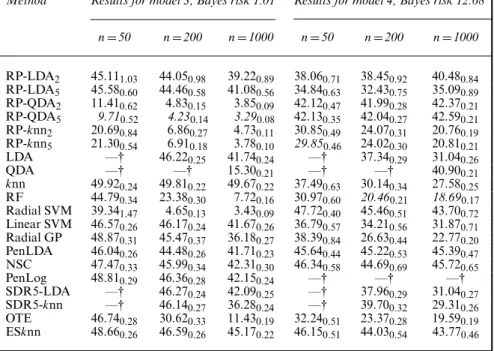
Fig. 3 illustrates ˆπ1Gˆn,1.α/+πˆ0{1−Gˆn,0.α/} as an estimator of π1Gn,1.α/+π0{1−
Gn,0.α/}, for the QDA base classifier and for various values ofnandπ1. Here, a very good
approximation to the estimand was obtained by using an independent data set of size 5000.
Unsurprisingly, the performance of the estimator improves asnincreases, but the most notable
feature of these plots is the fact that, for all classifiers and even for small sample sizes, ˆαis an
excellent estimator ofαÅand may be a substantial improvement on the naive choice ˆα=12(or
the appropriate prior weighted choice), which may result in a classifier that assigns every point to a single class.
5.3. Choice ofB1andB2
To minimize the Monte Carlo error as described in theorem 1 and proposition 1, we should
chooseB1to be as large as possible. The constraint, of course, is that the computational cost of
the random-projection classifier scales linearly withB1. The choice ofB2is more subtle; whereas
the third term in the bound in theorem 3 decreases asB2increases, we saw in Section 4 that
0.0 0.2 0.4 0.6 0.8 1.0 0.0 0.1 0.2 0.3 0.4 0.5 alpha (a) (b) (c) (d) (e) (f)
Objective function Objective function Objective function Objective function Objective function Objective function
0.0 0.2 0.4 0.6 0.8 1.0 0.0 0.1 0.2 0.3 0.4 0.5 alpha 0.0 0.2 0.4 0.6 0.8 1.0 0.0 0.1 0.2 0.3 0.4 0.5 alpha 0.0 0.2 0.4 0.6 0.8 1.0 0.0 0.1 0.2 0.3 0.4 0.5 0.6 alpha 0.0 0.2 0.4 0.6 0.8 1.0 0.0 0.1 0.2 0.3 0.4 0.5 0.6 alpha 0.0 0.2 0.4 0.6 0.8 1.0 0.0 0.1 0.2 0.3 0.4 0.5 0.6 alpha Fig. 3. π1 Gn ,1 . α 0/C π0 { 1 Gn ,0 . α 0/} in e xpression (5) ( ) and ˆ π1 ˆGn,1 . α 0/C ˆ π0 { 1 ˆGn ,0 . α 0/} ( ) for the QD A base classifier after projecting fo r one tr aining data set of siz e (a), (b) n D 50, (c), (d) n D 200 and (e), (f) n D 1000 from model 3 with (a), (c), (e) π1 D 0. 5 and (b), (d), (f) π1 D 0. 66: here , p D 100 and d D 2
that are given in theorem 3 and Section 4 to chooseB2to minimize the overall upper bound onE{R.CRPn /}−R.CBayes/. In practice, however, we found that an involved approach such as
this was unnecessary, and that the ensemble method was robust to the choice ofB1andB2; see
Section 3 of the on-line supplementary material for numerical evidence and further discussion.
On the basis of this numerical work, we recommendB1=500 andB2=50 as sensible default
choices, and indeed these values were used in all of our experiments in Section 6 as well as section 4 in the supplementary material.
5.4. Choice ofd
We want to choosed as small as possible to obtain the best possible performance bounds as
described in Section 4. This also reduces the computational cost. However, the performance
bounds rely on assumption 3, whose strength decreases asdincreases, so we want to choosed
sufficiently large that this condition holds (at least approximately).
In Section 6 we see that the random-projection ensemble method is quite robust to the choice
ofd. Nevertheless, in some circumstances it may be desirable to have an automatic choice, and
cross-validation provides one possible approach when computational cost attraining timeis not
too constrained. Thus, if we wish to choosedfrom a setD⊆{1,: : :,p}, then for eachd∈Dwe
train the random-projection ensemble classifier and set ˆ
d:=sarg min
d∈D
[ ˆπ1Gˆn,1.αˆ/+πˆ0{1−Gˆn,0.αˆ/}],
where ˆα=αˆdis given in expression (17). Such a procedure does not add to the computational
cost attest time. This strategy is most appropriate when max{d:d∈D}is not too large (which
is the setting that we have in mind); otherwise a penalized risk approach may be more suitable.
6. Empirical analysis
In this section, we assess the empirical performance of the random-projection ensemble classifier
in simulated and real data experiments. We shall write RP-LDAd, RP-QDAd and RP-knndto
denote the random-projection classifier with LDA, QDA andknn respectively; the subscriptd
refers to the dimension of the image space of the projections.
For comparison we present the corresponding results of applying, where possible, the three
base classifiers (LDA, QDA,knn) in the originalp-dimensional space alongside 11 other
clas-sification methods chosen to represent the state of the art. These include RFs (Breiman, 2001); SVMs (Cortes and Vapnik, 1995), Gaussian process (GP) classifiers (Williams and Barber, 1998) and three methods designed for high dimensional classification problems, namely penalized LDA, PenLDA (Witten and Tibshirani, 2011), nearest shrunken centroids (NSCs) (Tibshirani et al., 2003) andl1-penalized logistic regression, PenLog (Goemanet al., 2015).
A further comparison is with LDA andknn applied after a single projection chosen on the
basis of the sufficient dimension reduction assumption, SDR5. For this method, we project
the data into five dimensions by using the proposal of Shinet al.(2014). This method requires
n > p. Finally, we compare with two related ensemble methods: optimal tree ensembles (OTEs)
(Khanet al., 2015a) and ensemble of subset ofk-nearest-neighbour classifiers, ESknn (Gulet al.,
2016).
Many of these methods require tuning parameter selection, and the parameters were chosen as
follows: for theknn standard classifier, we chosekvia leave-one-out cross-validation from the set
{3, 5, 7, 9, 11}. RF was implemented by using therandomForestpackage (Liaw and Wiener,
package) components randomly selected when training each tree. For the radial SVM, we used
the reproducing basis kernelK.u,v/:=exp{−.1=p/u−v2}. Both SVM classifiers were
imple-mented by using thesvmfunction in thee1071package (Meyeret al., 2015). The GP classifier
uses a radial basis function, with the hyperparameter chosen via the automatic method in the gaussprfunction in thekernlabpackage (Karatzoglouet al., 2015). The tuning parameters for the other methods were chosen using the default settings in the corresponding R packages PenLDA(Witten, 2011),NSC(Hastieet al., 2015) andpenalized(Goemanet al., 2015) namely
sixfold, tenfold and fivefold cross-validation respectively. For the OTE and ESknn methods we
used the default settings in the R packagesOTE(Khanet al., 2015b) andESKNN(Gulet al.,
2015).
6.1. Simulated examples
We present four simulation settings which were chosen to investigate the performance of the random-projection ensemble classifier in a wide variety of scenarios. In each of the examples
below, we taken∈{50, 200, 1000}andp∈{100, 1000}and investigate two different values of
the prior probability. We use Gaussian projections (see Section 5.1) and setB1=500 andB2=50
(see Section 5.3).
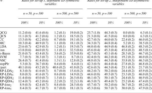
The risk estimates and standard errors for thep=100 andπ1=0:5 case are shown in Tables
1 and 2 (the remaining results are given in the on-line supplementary material). These were
calculated as follows: we setntest=1000 andNreps=100, and forl=1,: : :,Nrepswe generate
a training set of size nand a test set of sizentest from the same distribution. Let ˆRl be the
proportion of the test set that is classified incorrectly in thelth repeat of the experiment. The
overall risk estimate presented isrisk : =.1=Nreps/ΣNl=reps1 Rˆl. Note that
Table 1. Misclassification rates for models 1 and 2, withpD100 andπ1D0.5
Method Results for model 1, Bayes risk 4.45 Results for model 2, Bayes risk 4.09
n=50 n=200 n=1000 n=50 n=200 n=1000 RP-LDA2 49:340:26 48:100:31 44:140:46 8:340:28 5.560:12 5.170:10 RP-LDA5 49:810:24 48:860:30 46:910:40 8.170:27 5.640:13 5.140:10 RP-QDA2 44:180:29 29:380:49 10:570:22 8:400:29 5.570:12 5.160:10 RP-QDA5 39:320:33 22.320:32 8.750:15 8.060:25 5.580:12 5.090:10 RP-knn2 46:100:30 36:180:32 19:420:20 8:940:36 5.600:12 5:200:10 RP-knn5 43:650:30 25:340:35 10:210:16 9:000:33 5.680:12 5.130:10 LDA —† 49:600:23 49:910:22 —† 14:320:22 6:340:11 QDA —† —† 27:360:23 —† —† 17:100:20 knn 34.660:35 23:710:31 15:310:17 12:810:28 8:800:15 7:280:13 RF 49:720:23 48:330:25 43:280:43 11:110:31 6:800:12 6:070:11 Radial SVM 49:830:22 50:160:22 48:670:22 24:041:47 6:370:14 5:460:10 Linear SVM 50:020:23 49:550:21 50:040:22 9:410:21 8:960:17 7:760:13 Radial GP 48:180:30 42:760:29 26:600:24 14:090:63 5:840:13 5.090:10 PenLDA 49:950:23 49:790:23 50:050:22 11:110:55 6:720:20 5:790:12 NSC 49:740:23 49:690:26 49:550:24 12:610:61 7:270:28 5:820:13 PenLog 49:660:35 49:880:24 50:120:21 11:370:22 7:670:14 6:000:11 SDR5-LDA —† 37:800:48 35:310:30 —† 15:070:22 6:470:11 SDR5-knn —† 32:220:71 21:831:08 —† 18:810:29 7:750:12 OTE 48:510:33 34:731:23 9:570:66 18:260:47 12:440:26 9:240:15 ESknn 50:130:23 49:870:22 49:770:21 40:300:71 37:060:63 32:980:58 †Not applicable.
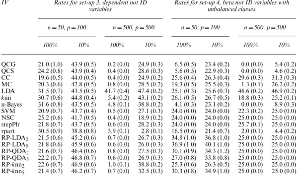
Table 2. Misclassification rates for models 3 and 4, withpD100 andπ1D0.5
Method Results for model 3, Bayes risk 1.01 Results for model 4, Bayes risk 12.68
n=50 n=200 n=1000 n=50 n=200 n=1000 RP-LDA2 45:111:03 44:050:98 39:220:89 38:060:71 38:450:92 40:480:84 RP-LDA5 45:580:60 44:460:58 41:080:56 34:840:63 32:430:75 35:090:89 RP-QDA2 11:410:62 4:830:15 3:850:09 42:120:47 41:990:28 42:370:21 RP-QDA5 9.710:52 4.230:14 3.290:08 42:130:35 42:040:27 42:590:21 RP-knn2 20:690:84 6:860:27 4:730:11 30:850:49 24:070:31 20:760:19 RP-knn5 21:300:54 6:910:18 3:780:10 29.850:46 24:020:30 20:810:21 LDA —† 46:220:25 41:740:24 —† 37:340:29 31:040:26 QDA —† —† 15:300:21 —† —† 40:900:21 knn 49:920:24 49:810:22 49:670:22 37:490:63 30:140:34 27:580:25 RF 44:790:34 23:380:30 7:720:16 30:970:60 20.460:21 18.690:17 Radial SVM 39:341:47 4:650:13 3:430:09 47:720:40 45:460:51 43:700:72 Linear SVM 46:570:26 46:170:24 41:670:26 36:790:57 34:210:56 31:870:71 Radial GP 48:870:31 45:470:37 36:180:27 38:390:84 26:630:44 22:770:20 PenLDA 46:040:26 44:480:26 41:710:23 45:640:44 45:220:53 45:390:47 NSC 47:470:33 45:990:34 42:310:30 46:340:58 44:690:69 45:720:65 PenLog 48:810:29 46:360:28 42:150:24 —† —† —† SDR5-LDA —† 46:270:24 42:090:25 —† 37:960:29 31:040:27 SDR5-knn —† 46:140:27 36:280:24 —† 39:700:32 29:310:26 OTE 46:740:28 30:620:33 11:430:19 32:240:51 23:370:28 19:590:19 ESknn 48:660:26 46:590:26 45:170:22 46:150:51 44:030:54 43:770:46 †Not applicable. E.risk/=E{R.CnRP/} and var.risk/= 1 Nrepsvar.R1/ˆ = 1 Nreps E E{R.CnRP/}[1−E{R.CRPn /}] ntest +var[E{R.CRPn /}] :
We therefore estimate the standard error in the tables below by ˆ σ:= 1 Nreps1=2 risk.1−risk/ ntest + ntest−1 ntestNreps Nreps l=1 .Rˆl−risk/2 1=2 :
The method with the smallest risk estimate in each column of the tables below is highlighted in italics; where applicable, we also highlight any method with a risk estimate within 1 standard error of the minimum.
6.1.1. Sparse class boundaries: model 1
Here, X|{Y=0}∼12Np.μ0,Σ/+12Np.−μ0,Σ/, and X|{Y=1}∼12Np.μ1,Σ/+12Np.−μ1,Σ/,
where, forp=100, we setΣ=I100×100,μ0=.2,−2, 0,: : :, 0/Tandμ1=.2, 2, 0,: : :, 0/T.
In model 1, assumption 3 holds withd=2; for example, we could take the rows ofAÅ to
be the first two Euclidean basis vectors. We see that the random-projection ensemble classifier with the QDA base classifier performs very well here, as does the OTE method. Despite the fact
that the regression functionη depends on only the first two components in this example, the comparators that were designed for sparse problems do not perform well; in some cases they are no better than a random guess.
6.1.2. Rotated sparse normal: model 2
Here, X|{Y=0}∼Np.Ωpμ0,ΩpΣ0ΩTp/, and X|{Y=1}∼Np.Ωpμ1,ΩpΣ1ΩTp/, where Ωp is a
p×protation matrix that was sampled once according to Haar measure, and remained fixed
thereafter, and we setμ0=.3, 3, 3, 0,: : :, 0/T andμ1=.0,: : :, 0/T. Moreover,Σ0andΣ1 are
block diagonal, with blocksΣ.1/
r , andΣ.r2/, forr=0, 1, whereΣ.
1/
0 is a 3×3 matrix with diagonal
entries equal to 2 and off-diagonal entries equal to21, andΣ.11/=Σ0.1/−I3×3. In both classesΣ.r2/
is a.p−3/×.p−3/matrix, with diagonal entries equal to 1 and off-diagonal entries equal to12.
In model 2, assumption 3 holds withd=3; for instance,AÅcan be taken to be the first three
rows ofΩTp. Perhaps surprisingly, whether we use too small a value ofd (namelyd=2), or a
value that is too large (d=5), the random-projection ensemble methods still classify very well.
6.1.3. Independent features: model 3
Here,P0=Np.μ,Ip×p/, withμ=.1=√p/.1,: : :, 1, 0,: : :, 0/T, whereμhasp=2 non-zero
com-ponents, whereas P1 is the distribution ofpindependent components, each with a standard
Laplace distribution.
In model 3, the class boundaries are non-linear and, in fact, assumption 3 is not satisfied for anyd < p. Nevertheless, in Table 2 we see that, where the LDA, QDA andknn classifiers are tractable, they are outperformed by their random-projection ensemble counterparts and in fact
the RP-QDA5classifier has the smallest misclassification rate among all methods implemented.
Unsurprisingly, the methods that are designed for a linear Bayes decision boundary are not effective. The RP-QDA classifiers are especially accurate here; in particular, they can cope better with the non-linearity of the class boundaries than the RP-LDA classifiers.
6.1.4. t-distributed features: model 4
Here,X|{Y=r}=μr+Zr=
√
.Ur=νr/, whereZr∼Np.0,Σr/independent ofUr∼χ2νr, forr=
0, 1, i.e. Pr is the multivariate t-distribution centred at μr, with νr degrees of freedom and
shape parameterΣr. We setμ0=.1,: : :, 1, 0,: : :, 0/T, whereμ0has 10 non-zero components,
μ1=0,ν0=2,ν1=1,Σ0=.Σj,k/, whereΣj,j=1,Σj,k=0:5 if max.j,k/10 andj=k,Σj,k=0
otherwise, andΣ1=Ip×p.
Model 4 explores the effect of heavy tails and the presence of correlation between the features.
Again, assumption 3 is not satisfied for anyd < p. The RF, OTE and RP-knn methods all perform
very well here. The RP-LDA and RP-QDA classifiers are less good. This is partly because the class conditional distributions do not have finite second and first moments respectively and, as a result, the class mean and covariance matrix estimates are poor.
6.2. Real data examples
In this section, we compare the classifiers above on eight real data sets that are available from the University of California Irvine Machine Learning Repository. In each example, we first
subsample the data to form a training set of sizenand then use the remaining data (or, where
available, take a subsample of size 1000 from it) to form the test set. As with the simulated
examples, we setB1=500 and B2=50 and used Gaussian-distributed projections, and each
Table 3. Misclassification rates for the eye state and ionosphere data sets
Method Results for eye state data Results for ionosphere data
n=50 n=200 n=1000 n=50 n=100 n=200 RP-LDA5 42:060:38 38:610:29 36:300:21 13:050:38 10:750:25 9:780:26 RP-QDA5 38.970:39 32:440:42 30:910:87 8.140:37 6.150:22 5.210:20 RP-knn5 39.370:39 26.910:27 13.540:19 13:050:46 7:430:25 5:430:19 LDA 42:380:40 39:150:30 36:910:23 23:720:40 18:270:28 15:580:31 QDA 39:910:35 29:240:40 29:761:07 —† —† 14:070:34 knn 41:700:40 29:180:27 14:450:16 21:810:73 18:050:46 16:400:35 RF 39.270:37 29:040:25 17:630:20 10:520:30 7:540:19 6:480:18 Radial SVM 46:330:49 38:710:46 31:030:68 27:671:15 12:850:91 6:670:22 Linear SVM 42:380:42 39:550:36 38:580:38 19:410:35 17:050:27 15:480:29 Radial GP 40:730:38 32:220:25 21:660:21 22:290:72 17:810:46 14:520:31 PenLDA 44:370:43 42:500:28 41:860:23 21:200:57 19:830:56 19:810:54 NSC 44:730:48 42:370:29 42:270:28 22:620:53 19:110:42 17:520:34 SDR5-LDA 42:820:40 39:250:29 36:920:23 25:780:52 18:980:30 15:630:30 SDR5-knn 42:430:38 34:130:32 25:310:25 30:610:74 17:530:45 10:120:30 OTE 40:100:38 29:920:28 18:730:20 14:380:41 9:800:27 7:330:23 ESknn 45:620:41 43:060:35 39:370:34 27:810:58 23:230:48 20:050:51 †Not applicable.
the methods that were described at the beginning of Section 6 for each of the 100 repeats of the experiment.
6.2.1. Eye state detection
The electroencephalogram eye state data set (http://archive.ics.uci.edu/ml/
datasets/EEG+Eye+State) consists of p=14 electroencephalogram measurements on 14 980 observations. The task is to use the electroencephalogram reading to determine the state of the eye. There are 8256 observations for which the eye is open (class 0), and 6723 for which the eye is closed (class 1). Results are given in Table 3.
6.2.2. Ionosphere data set
The ionosphere data set (http://archive.ics.uci.edu/ml/datasets/Ionosph
ere) consists ofp=32 high frequency antenna measurements on 351 observations.
Obser-vations are classified as good (class 0) or bad (class 1), depending on whether there is evidence for free electrons in the ionosphere or not. The class sizes are 225 (good) and 126 (bad). Results are given in Table 3.
6.2.3. Down’s syndrome diagnoses in mice
The mice data set (http://archive.ics.uci.edu/ml/datasets/Mice+Protein+
Expression) consists of 570 healthy mice (class 0) and 507 mice with Down’s syndrome
(class 1). The task is to diagnose Down’s syndrome on the basis ofp=77 protein expression
measurements. Results are given in Table 4. 6.2.4. Hill–valley identification
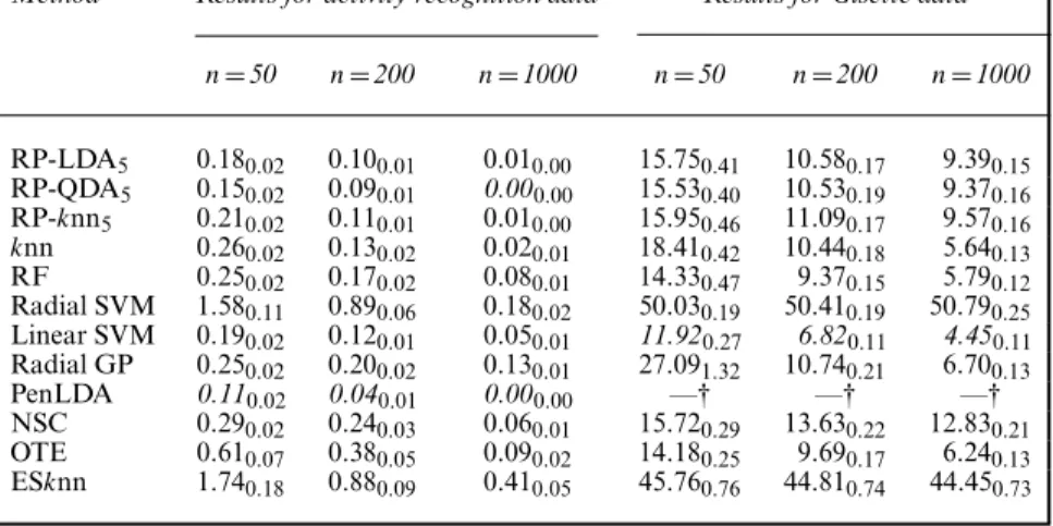
Table 4. Misclassification rates for the mice and hill–valley data sets
Method Results for mice data Results for hill–valley data
n=200 n=500 n=1000 n=100 n=200 n=500 RP-LDA5 25:170:30 23:560:26 23:350:49 36.840:84 36.450:85 32.571:06 RP-QDA5 18:240:29 16:050:24 15:450:45 44:430:34 43:560:31 41:100:33 RP-knn5 11:240:29 2.240:10 0.550:09 49:080:24 47:270:26 36:390:29 LDA 6.460:14 3:380:10 2:170:17 —† 37:290:48 34:370:36 knn 19:650:26 7:020:17 0:940:13 49:350:24 48:820:21 47:490:24 RF 7:940:22 2:410:11 0.510:08 48:320:23 47:230:21 44:110:25 Radial SVM 11:250:29 3:890:13 1:690:16 50:240:19 50:240:19 50:420:21 Linear SVM 6.360:14 3:640:10 2:510:17 48:560:22 47:030:23 44:840:28 Radial GP 21:220:30 13:780:24 8:660:34 48:330:22 47:240:21 45:110:22 PenLDA 26:100:36 24:070:26 23:910:46 49:590:22 49:730:21 49:550:22 NSC 30:300:36 28:060:29 28:470:51 49:870:21 49:910:20 49:920:22 OTE 11:830:32 6:260:18 3:260:23 48:330:23 47:180:22 44:200:24 ESknn 39:030:59 34:330:66 31:650:78 49:310:23 48:900:23 48:030:25 †Not applicable.
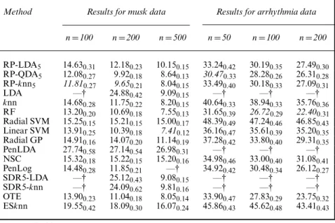
Table 5. Misclassification rates for the musk and cardiac arrhythmia data sets
Method Results for musk data Results for arrhythmia data
n=100 n=200 n=500 n=50 n=100 n=200 RP-LDA5 14:630:31 12:180:23 10:150:15 33:240:42 30:190:35 27:490:30 RP-QDA5 12:080:27 9:920:18 8:640:13 30.470:33 28:280:26 26:310:28 RP-knn5 11.810:27 9.650:21 8:040:15 33:490:40 30:180:33 27:090:31 LDA —† 24:880:42 9:090:15 —† —† —† knn 14:680:28 11:750:22 8:200:15 40:640:33 38:940:33 35:760:36 RF 13:200:20 10:690:18 7:550:13 31:650:39 26.720:29 22.400:31 Radial SVM 15:250:15 15:210:15 15:000:17 48:390:49 47:240:46 46:850:43 Linear SVM 13:910:25 10:390:18 7.410:12 36:160:47 35:610:39 35:200:35 Radial GP 14:910:16 14:070:20 11:140:19 37:280:42 33:800:40 29:310:35 PenLDA 27:740:58 27:140:54 26:980:31 —† —† —† NSC 15:320:18 15:220:15 15:200:16 34:980:46 33:000:40 31:080:41 PenLog 14:480:28 11:850:21 —† 34:920:42 30:480:34 26:120:27 SDR5-LDA —† 25:120:43 9:080:15 —† —† —† SDR5-knn —† 24:090:62 9:810:16 —† —† —† OTE 13:900:23 11:040:18 8:050:14 33:900:47 27:830:29 23:750:32 ESknn 19:550:42 18:090:30 16:070:24 45:860:43 45:620:48 43:410:43 †Not applicable.
consists of 1212 observations of a terrain, each when plotted in sequence represents either a hill (class 0; size 600) or a valley (class 1; size 612). The task is to classify the terrain on the basis of
a vector of dimensionp=100. Results are given in Table 4.
6.2.5. Musk identification
The musk data set (http://archive.ics.uci.edu/ml/datasets/Musk+\%28Ver
sion+2\%29) consists of 1016 musk (class 0) and 5581 non-musk (class 1) molecules. The task is
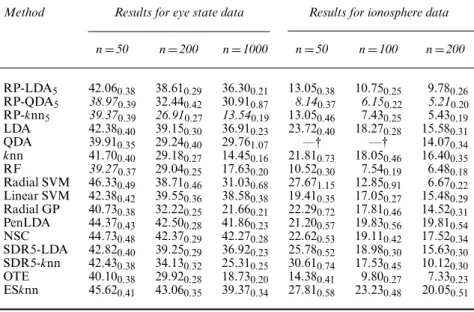
![Fig. 4. Relative discriminatory power, as a function of the angle θ 2 [0, π] for case 1 ( ) and case 2](https://thumb-us.123doks.com/thumbv2/123dok_us/817189.2603318/45.727.179.545.710.904/fig-relative-discriminatory-power-function-angle-case-case.webp)
