A Dynamic Multiobjective Evolutionary Algorithm
Based on A Dynamic Evolutionary Environment Model
Juan Zoua,∗, Qingya Lia, Shengxiang Yangc, Jinhua Zhenga,b, Zhou Penga,
Tingrui Peia
a
Key Laboratory of Intelligent Computing and Information Processing (Ministry of Education), Xiangtan University, Xiangtan 411105, China
b
Hunan Provincial Key Laboratory of Intelligent Information Processing and Application, Hengyang Normal University, Hengyang 421002, China
c
School of Computer Science and Informatics, De Montfort University, Leicester LE1 9BH, U.K.
Abstract
Traditional dynamic multiobjective evolutionary algorithms usually imitate the evolution of nature, maintaining diversity of population through different strate-gies and making the population track the Pareto optimal solution set efficiently after the environmental change. However, these algorithms neglect the role of the dynamic environment in evolution, leading to the lacking of active guided search. In this paper, a dynamic multiobjective evolutionary algorithm based on a dynamic evolutionary environment model is proposed (DEE-DMOEA). When the environment has not changed, this algorithm makes use of the evolutionary environment to record the knowledge and information generated in evolution, and in turn, the knowledge and information guide the search. When a change is detected, the algorithm helps the population adapt to the new environment through building a dynamic evolutionary environment model, which enhances the diversity of the population by the guided method, and makes the environ-ment and population evolve simultaneously. In addition, an impleenviron-mentation of the algorithm about the dynamic evolutionary environment model is introduced in this paper. The environment area and the unit area are employed to express
∗Corresponding author
Email addresses: [email protected] (Juan Zou),[email protected](Qingya Li),[email protected](Shengxiang Yang),[email protected](Jinhua Zheng),
the evolutionary environment. Furthermore, the strategies of constraint, facili-tation and guidance for the evolution are proposed. Compared with three other state-of-the-art strategies on a series of test problems with linear or nonlinear correlation between design variables, the algorithm has shown its effectiveness for dealing with the dynamic multiobjective problems.
Keywords: Dynamic multiobjective optmization, evolutionary algorithms, evolutionary environment, dynamic evolutionary environment model
1. Introduction
Many real-world problems are dynamic multiobjective optimization prob-lems (DMOPs), with conflicts among multiple objectives as well as objective functions that change over time [1]. Tracking the Pareto optimal solution set after a change is an important and challenging issue. On these issues, the researched objectives often change intricately with time. The goal of the tra-ditional evolutionary algorithms is to make the population gradually converge to get a satisfactory solution set, but this makes the population lose diversity. Especially, in the later stages of the evolution, the population will gradually lose the ability to adapt to the environmental changes, which is a challenge of the traditional evolutionary algorithms in the dynamic environment [2, 3, 24, 4, 5]. In order to track the optimal solution set in a timely manner after a change, researchers need to make some adjustments on the traditional static multiobjec-tive algorithms [6, 7, 8, 9], so that they can quickly respond to the environmental changes.
In recent years, researchers have designed many new ways to solve DMOPs on the basis of static algorithms [10, 11, 13, 14, 16, 17, 18, 19, 20, 21], such as random initialization [12, 25, 26, 18, 17], hyper mutation [25, 22, 15, 33], mem-ory [25, 26, 29, 30, 36, 23, 41], and prediction [31, 32, 33, 34, 35, 36, 42, 48, 49]. These strategies have been proven effective for solving DMOPs; however, they are defective in the following ways. Firstly, random initialization, hyper muta-tion and dynamic migramuta-tion strategies are all a blind way to enhance populamuta-tion
diversity without a right guidance, and the performance of convergence is un-satisfactory when dealing with complex DMOPs. Secondly, memory strategy reuses the optimal solutions which are previously searched in the previous time to rapidly respond to changes in the new environment. This strategy can achieve good results for periodic problems. However, for non-periodic problems or in the first cycle of the changing environment, population is still in the process of blind evolution. Thus, the algorithm is difficult to obtain a good convergence. Lastly, methods that are based on prediction generate a new optimal solution set by the prediction model for the evolution of the population, and help the algorith-m to respond quickly to new changes. However, obtaining accurate predictions remains a primary difficulty. Thus, designing a more accurate prediction model is still a focus of the present research.
To solve these problems, on the premise of less history information and utilizing the characteristics of the evolutionary environment itself, the paper proposes a dynamic multiobjective evolutionary algorithm based on a dynamic environment evolutionary model, referred to as DEE-DMOEA. Current dynamic multiobjective optimization algorithms do not consider the role of the dynamic environment for the evolutionary population. Actually, the effect of the environ-ment on evolutionary individuals is very important, for individuals must survive and evolve in a specific environment. The wonderful interaction between the natural environment and the biology that makes biomass have such a present perfect structure. Therefore, how to research from the perspective of the dy-namic environment, using the dydy-namic environmental knowledge to guide the evolution of population in the new environment to accelerate convergence of the population is the research focus in this paper.
The rest of the paper is organized as follows. Section 2 provides important terminology. Section 3 describes the dynamic environment evolutionary model. Section 4 describes the implementation of the evolutionary model. Section 5 introduces the test problems and evaluation metrics. Section 6 gives the ex-perimental results and analysis. Section 7 provides the conclusions and future work.
2. Background
A minimization problem is considered here without loss of generality. The dynamic multiobjective optimization problem [1] can be described as:
min xǫΩF(x, t) = (f1(x, t), f2(x, t), . . . , fm(x, t)) T s.t. gi(x, t)≤0i= 1,2, ..., p; hj = 0j = 1,2, ..., q
wheretis the time variable andx= (x1, x2, . . . , xn) is the n-dimensional decision
vector bounded by the decision space Ω. F = (f1, f2, . . . , fm) presents the set
ofmobjectives to be minimized and the functions of gi≤0i= 1,2, . . . , p and hj = 0j= 1,2, . . . , qpresent the set of inequality and equality constraints.
Definition 1 (Pareto Dominance). p and q are any two individuals in the
population;pis said to dominate q, denoted byf(p)≺f(q) if f fi(p)≤fi(q)
∀i={1,2, . . . , m} andfj(p)< fj(q)∃j∈ {1,2, . . . , m}.
Definition 2 (Pareto Optimal Set(PS)). x is the decision variable; Ω is
the decision space; F is the objective function; thus, the PS [7] is the set of all non-dominated solutions and is defined mathematically as:
P S:={x∈Ω|6 ∃x⋆∈Ω, F(x⋆)≺F(x)}
Definition 3 (Pareto Optimal Front(PF)). xis the decision variable;F is
the objective function; thus, the PF [7] is the set of non-dominated solutions with respect to the objective space and is defined mathematically as:
P F :={y=F(x)|x∈P S}
3. Dynamic Environment Evolutionary Model
In ecology, environment refers to external matters such as the surrounding ecosystem which affects biological communities. In our dynamic environment evolutionary model, the environment refers to a group of entities which can guide and promote the evolution of the population. Especially, after environmental
changes, it can guide the evolution and convergence of the population in the new environment.
An evolutionary population must survive and evolve in a specific environ-ment. The environment plays constraint, facilitating and guiding roles for the evolution of the population, and these three environmental roles are completely different. Constraint is mainly used to ensure the legitimacy of individuals; fa-cilitating is mainly used to enhance the efficiency of the evolution and improve the distribution of evolutionary population. Guiding is mainly used to help the population adapt to the new environment. At the same time, the evolu-tionary population is counteractive to the evoluevolu-tionary environment, which is mainly shown in the impact on the attributes of the evolutionary environment, such as the changes of the current evolutionary state and the update of the environmental knowledge.
In a dynamic environment, how to maintain the diversity of the popula-tion after an environmental change is the key to solve DMOPs. When the environment changes, environmental information and knowledge make a differ-ence. Making full use of this information in a dynamic environment to help the population adapt to the new environment plays an important role for solving DMOPs.
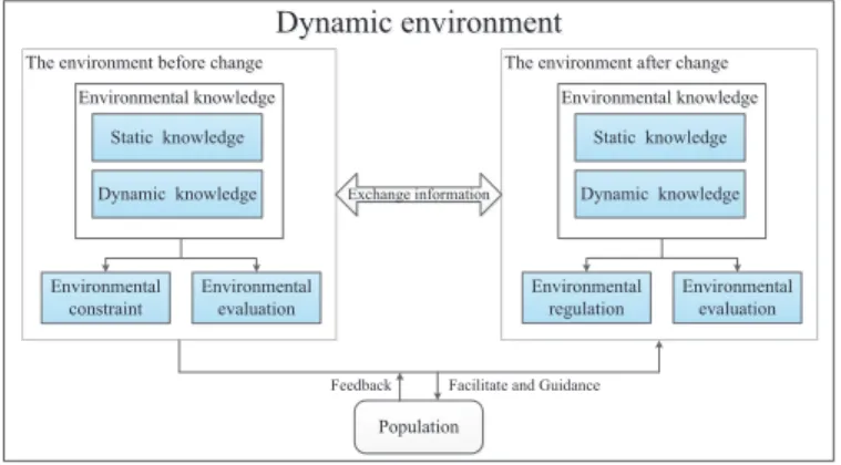
Fig. 1 shows a general framework of a dynamic evolutionary environment model. A dynamic environment model consists of two different kinds of en-vironment before and after the enen-vironmental change. Enen-vironment elements include environmental knowledge, environmental evaluation, environmental con-straint before change and environmental regulation after change. Among them, environmental knowledge can be divided into static knowledge and dynamic knowledge. Static knowledge is the preset environmental attributes which main-tain constant values in the process of evolution, such as environmental capacity and dimensions. Dynamic knowledge is the environmental attributes which are affected by population in the process of environmental change, such as the con-gestion degree, the domain to be oriented, direction of environmental change and newly generated individuals for guiding evolution. the environmental
eval-uation mechanism evaluates the living conditions of the population or individ-uals according to environmental knowledge, such as individual location in the environment and the entire population distribution.
Environmental constraint before change mainly includes two parts: 1) the satisfaction constraint of the expected solution set, and 2) the distribution con-straint of the expected solution set. Environmental concon-straint mostly reflects on the guidance for the population, that is to say, it can achieve the evolution in the environment by environmental constraint.
Environmental regulation after change means that individuals need to make the corresponding change in order to adapt to the new environment. There are two different kinds of environment exchange information to facilitate and guide the evolution of the population. In return, the population will send the feedback information which is generated in the process of evolution to the environment, updating the environmental knowledge and achieving co-evolution.
The dynamic environmental facilitating and guiding mechanism for the pop-ulation is the core of DEE-DMOEA, which determines the evolutionary direc-tion of the populadirec-tion and plays a decisive motivadirec-tional role in the evoludirec-tion. The dynamic environmental facilitating mechanism indicates that, when the environment does not change, on the one hand, it promotes the individual ac-celerated evolution in compliance with environmental satisfaction constraints. On the other hand, it balances the density of population distribution and ex-pands the range of population distribution in compliance with the environmental distribution constraints. The dynamic environmental guiding mechanism aims to enhance population diversity by guided method according to environmental regulation after change, help population adapt to the new environment, and accelerate the algorithm to quickly track the new Pareto optimal solution set.
4. Implementation of The Evolutionary Model
Each individual in a dynamic environment has a living space. Here we use a mechanism which is similar to the grid, referred to as the environment
Dynamic environment Dynamic environment he environment befoff re change
The environment before change The environment aftThe environment after changeff er change Environmental knowledge Environmental knowledge Static knowledge Dynamic knowledge Environmental knowledge Environmental knowledge Environmental evaluation Static knowledge Dynamic knowledge Environmental regulation Population
Feedback Facilitate and Guidance Exchange information
Environmental evaluation Environmental
constraint
Figure 1: A general framework of dynamic environment evolutionary model.
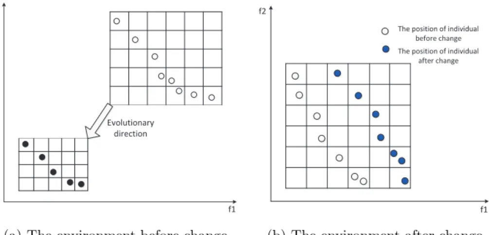
domain, to store the individuals in the dynamic environment. The environment domain consists of many identical grids, which are called the unit domains. The dimensions of the environment domain and unit domains are the same as the objective dimensions. The position of an individual in the environment domain will change accordingly when the environment changes. Therefore, in a dynamic environment, as shown in Fig. 2, when the environment does not change, the range of environment domain and the size of unit domain are determined by the location and distribution of population in the environment; the environment domain will constantly adjust with the evolution of the population. When the environment changes, the range of environment domain and the size of unit domain are co-determined by the different distributions of the population before and after the environmental change.
Bottom and top boundaries of each dimension in the environment domain are calculated as follows:
lbi=min(Pi)−(max(Pi)−min(Pi)/(2×num)) ubi=max(Pi) + (max(Pi)−min(Pi)/(2×num))
(1)
wherenum is the number of unit domains on each dimension in the objective space. The higher the objective dimension, the smaller the value ofnum. For example,numcan be set to 40 for two objectives and can be set to 10 for three
Evolutionary direction f1 f2 f1 f2
The position of individual before change The position of individual
after change
(a) The environment before change (b) The environment after change
Figure 2: Two different types of environment.
min(pi) max(pi)
lbi
lbi ubi
num= 5
Figure 3: The environment domain set on i-dimensional objective.
objectives. When the environment does not change, min(Pi) and max(Pi) denote the minimum and maximum values of the ith objective of population P. While a change is detected, min(Pi) andmax(Pi) denote the minimum and maximum values of theith objective of populationP in the two different kinds of environments before and after change, namely min(P.oldFi, P.newFi) and
max(P.oldFi, P.newFi). As shown in Fig. 3, the size of unit domain on theith
objective isarea sizei= (ubi−lbi)/num.
In a dynamic environment, when the environment does not change, each individual belongs to a specific unit domain. We denoteindiv.areaas the unit domain to which individual indiv belongs. According to the boundary of the environment domain and the size of unit domain, the unit domain position (do-main coordinate) of each individual can be determined. The do(do-main coordinate
ofindiv.areaon thei-th objective dimension can be calculated as Eq. (2).
indiv.areai=⌊(indiv.Fi−lbi)/area sizei⌋ (2)
where indiv.Fi is the i-th objective value of individual indiv. In Eq. (1) of calculatinglbi,min(Pi) andmax(Pi) denote the minimum and maximum values of theith objective of populationP.
While the environment changes, each individual may belong to two different unit domains before and after the environmental change, at this time the en-vironment domain will be reconstructed. Therefore, we denoteindiv.old area as the unit domain to which individualindiv belongs before the environmental change andindiv.new area as the unit domain to which individual indiv be-longs after the environmental change. The domain coordinates ofindiv.old area
andindiv.new areaon the i-th objective can be calculated as follows:
indiv.old areai=⌊(indiv.oldFi−lbi)/area sizei⌋
indiv.new areai=⌊(indiv.newFi−lbi)/area sizei⌋
(3)
where indiv.oldFi and indiv.newFi are respectively the i-th objective values before and after an environmental change. In Eq. (1) of calculatinglbi,min(Pi) and max(Pi) denote the minimum and maximum values of thei-th objective of populationP in the two different kinds of environments before and after a change.
The environment domain and unit domain have been set, then the various elements of composing dynamic environment and their implementation will be introduced.
4.1. Environmental Knowledge
Environmental knowledge is an important part of the environment, which de-notes the information recorded in the current dynamic environment. In our ap-proach, environmental knowledge is divided into two types: the environment do-main knowledge and unit dodo-main knowledge. The environment dodo-main knowl-edge is divided into static and dynamic environment domain knowlknowl-edge. Static
environment domain knowledge includes environmental capacity, the number of unit domains on each dimension and other preset environmental attributes. Dy-namic environment domain knowledge includes the bottom boundary and top boundary of the environment domain on each dimension, the size of unit do-main, the number of unit domains containing any individuals, the domain to be oriented, the direction of environmental change, the newly generated individuals for guiding the evolution, and other environmental attributes which are affected by the population. The new individuals are a series of re-initialized individuals to help the population adapt to the new environment after an environmental change and accelerate the convergence of the population and individuals, which will be described in detail in Section 4.3.
Unit domain knowledge is dynamic knowledge, which includes the number of individuals in each unit domain, a representative individual and the non-dominated unit domains. Representative individual is the optimal individual in a unit domain. Here, we set the individual with the nearest Euclidean distance to the origin of unit domain as the representative individual. The origin of the unit domain is the minimum on each dimension.
4.2. Environmental Constraint
When the environment does not change, survival and evolution of each in-dividual in the environment domain are required to meet the satisfaction con-straint; not all offspring generated by evolution can enter the environment do-main. Here, we stipulate that the individual in the environment domain must satisfy the following two constraints:
1) Individuals in each unit domain of the environment domain are mutually non-dominated.
2) Unit domains in the environment domain must be mutually domain strong non-dominated. The unit domain here refers to the unit domain containing any individual.
3) The strong dominance relation is stricter than the Pareto dominance. The domain strong dominance relation is defined as follows.
Definition 4 (Domain strong dominance). AandB are any two unit
do-mains in the environment domain; A is said to domain strong dominate B, denoted byA≺≺areaB if A.areai< B.areai∀i={1,2, . . . , r}. Where r is the
dimensions of the unit domain.
Similarly, the domain dominance can be defined as follows:
Definition 5 (Domain dominance). C andD are any two unit domains in
the environment domain,Cis said to domain dominate D, denoted byC≺area
D if f C.areai ≤ D.areai∀i = {1,2, . . . , r} and C.areaj < D.areaj ∃j ∈
{1,2, . . . , r}.
4.3. Environmental Evaluation
In a dynamic evolutionary environment model, the evaluation mechanism needs to evaluate not only the fitness of the population, but also the living con-ditions of the population and individuals according to environmental knowledge, and prepares for guiding evolution. The evaluation mechanism is divided into two types, one is evaluation for the individual, and the other is evaluation for the population.
Evaluation for the individual is to calculate the unit domain coordinates for each individual when the environment does not change according to Eq. (2), and to determine the representative individual. While the environment changes, the evaluation calculates two different unit domain coordinates for each indi-vidual, and provides feedback to the environment to construct a new dynamic environment.
Evaluation for the population first evaluates the distribution of the entire population in the new environment according to the environmental knowledge, then generates a new series of guide-individuals to prepare for guiding evolution.
The new guide-individuals are defined by Eq. (4): initt k=xtk+ Ckt−Ckt−1 Gaussian , if Ckt−Ckt−1>0 initt k=xtk− Ckt−Ckt−1 Gaussian , if Ckt−Ckt−1<0 (4) where xt
k is the individual at time t; k = 1,2, ..., n; n is the dimensions of the decision space. Gaussian is a random number generated from a standard normal distribution with mean 0 and variance 1, which has been verified in [27] to be a good strategy to enhance the ability of elaborate search. Ct
kis the center of non-dominated solutions obtained at timet, which can be defined by Eq. (5):
Ct k = 1 PNt −dominance X xt k xt kǫP t N−dominance (5) where PNt −dominance
is the size of non-dominated solutions.
Similarly, the domain coordinates of new guide-individuals are also calculat-ed.
In this way, we use the possible correlation between environmental changes to produce a series of guide-individuals. These individuals will be served as the alternative individuals in the process of environmental facilitating and guid-ing, to help the population adapt to the new environment and accelerate the convergence of population to the new PF.
4.4. Environmental Regulation
In a dynamic environment, different problems have different regulations. The location and distribution of the population in the new environment domain may not be suitable for its evolution and convergence. Therefore, the popu-lation needs to make the corresponding change in order to adapt to the new environment.
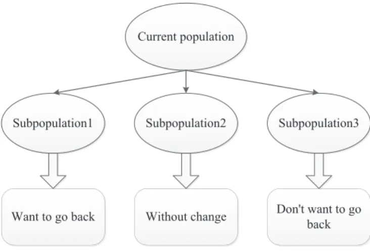
As shown in Fig. 4, just like people’s psychological reactions in real life, some individuals want to return to the past environment and continue to survive and evolve, considering that the environment before change is more conducive for evolution. While some individuals do not want to return to the past environ-ment, at the same time they are also confused about where they should go.
Current population
Subpopulation1 Subpopulation2 Subpopulation3
Want to go back Without change Don't want to go
back
Figure 4: The division of population.
There is also a group of individuals who do not want to make any change, they consider that the current environment is an ideal evolutionary environment.
Therefore, we need to divide the current population into three sub-populations according to the different behavioral characteristics of individuals when the en-vironment changes. Meanwhile, in order to maintain the distribution of sub-populations and avoid crowding the solution set, the three sub-sub-populations need to be more evenly divided. Sub-populations are divided as follows (illustrated by the example of two objectives):
The sizes of three sub-populations are respectively set tonum sub1,num sub2
andnum sub3 (Initially, for two objectives: 30, 40 and 30; for three objectives:
60, 80 and 60).
For the subpopulation2 which is without any change: we gather directly
num sub2 non-dominated individuals whose crowding-distance [44] is the largest
from the original population to subpopulation2.
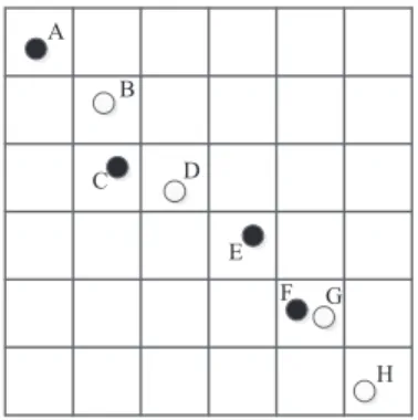
For the subpopulation1 which wants to go back and the subpopulation3 which does not want to go back: Algorithm 1 gives a detailed procedure of this strategy, where the domain-adjacent is defined as follows:
Algorithm 1SubpopulationDivision
Require: N D(population without division),q(picked individual)
1: for allq∈N Ddo
2: p:=q->next
3: for allP!=nulldo
4: flag:=false
5: if pis domain-adjacent withqthen
6: for allk∈N Ddo
7: if k.new area=p.new areathen
8: swap(p,q->next) 9: flag:=true 10: Break 11: end if 12: end for 13: if flag=falsethen 14: p:=p->next 15: end if 16: else 17: swap(p,q->next) 18: break 19: end if 20: end for 21: end for
22: Select the top num sub1 individuals in N D as subpopulation1, the rest of
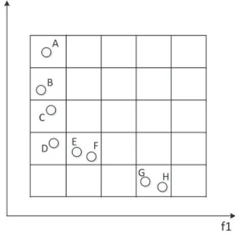
A B C D E F G H
Figure 5: An example about division of the sub-populations.
environment domain;U is domain-adjacent withV,if f |U.new areai−V.new areai| ≤
min dif f(i). min dif f(i) is the minimum difference on each dimension
be-tween any two unit domain coordinates. The unit domain here refers to the unit domain containing any individuals.
Fig. 5 is an example about division of the sub-populations. The first in-dividual A is selected, and then the second inin-dividual to compare with A is selected. The second individual is assumed to be B. Since B is domain-adjacent with A, and its unit domain does not include multiple individuals Therefore, B is discarded. Next, select the individual C, and C is not domain-adjacent with A, so C will be divided into the same sub-population with A and serves as the next individual for comparison. Similarly, E is not domain-adjacent with C and is divided into the same sub-population. Despite the fact that F is domain-adjacent with E, its unit domain includes another individual G, so F will be divided into the same subpopulation with A, C and E. Thus, the division ends. A, C, E and F are divided into the same sub-population. B, D, G and H are divided into another subpopulation.
It is worth noting that environmental regulation in this paper is clearly different from the random division of sub-populations such as charged PSO [37]. Environmental regulation considers the characteristics of different sub-populations to adapt to different environmental changes, and at the same time,
takes into account the distribution of the solution set, digging and using the environmental knowledge to guide the evolution.
4.5. Environmental Facilitating Mechanism
When the environment does not change, on the one hand, the environment facilitating mechanism promotes the individual accelerated evolution in compli-ance with environmental satisfaction constraints. On the other hand, it balcompli-ances the density of population distribution and expands the range of population dis-tribution in compliance with environmental disdis-tribution constraints. First, we introduce the accelerating action to promote evolution of the population. Classic multiobjective evolutionary algorithms typically recombine by randomly select-ing two or more individuals to achieve the evolution of population. However, this simple random selection will be hindered by the evolution to a certain exten-t. While two different individuals (especially non-dominated individuals) may generate far better offspring than parents which combines advantages of both parents after recombination. In the dynamic environment evolutionary model, we select more efficient individuals to recombine by giving the unit domain a relative fitness assignment. Relative to the unit domainAx1,x2,...,xr, the relative fitness of unit domainBy1,y2,...,yr is given as follows:
f(B)A= r X
i=1
Φ (xi, yi) (6)
where xi and yi are respectively the ith dimensional domain coordinates, and the definition of function Φ is given as follows:
Φ (xi, yi) = 1/(2 +yi−xi) xi≤yi xi−yi xi> yi (7)
Relative fitness is a relative concept, it does not represent the pros and cons of units in the environment domain. Relative to the unit domainA, the large relative fitness of unit domainB just indicates that selecting the individual in unit domainB and the individual in unit domainAto recombine will generate more excellent offspring than the parents. For instance, in Fig. 6, relative to the
f1 f2 A C D E F G H B
Figure 6: An illustration of individuals in the environment in a bi-objective space.
unit domain Area0,2, the relative fitness of domain Area0,4, Area0,3, Area0,1,
Area1,1 andArea3,0 are respectively 3/4, 5/6, 3/2, 4/3 and 11/5. The domain
coordinates of individual A in unit domainArea0,4is equal to the individual C
on the objectivef1, but two units larger on the objectivef2. So, it is difficult
to generate a much better individual than C in the process of recombination. That is to say, the promoting effect of A to C is not obvious. However, the domain coordinates of individual G or H in unit domainArea3,0 is three units
larger than the individual C on the objectivef1, but two units smaller on the
objectivef2. So, the generated offspring may inherit the different advantages of
parents, that is to say, the promoting effect of G or H to C is very powerful. For an individual to be recombined, we first select a unit domain according to the relative fitness by roulette, and then randomly select an individual within this unit to recombine with it. Here, we choose the SBX [38] and DE [39] operators to promote evolution.
Next, we introduce the balancing and expanding action to population distri-bution. The balancing and expanding action is mainly implemented by domain orientation. Domain orientation refers to generating new individuals in the do-main to be oriented, and meet the environmental distribution constraint. Here, we define the domain to be oriented as follows:
Definition 7 (The domain to be oriented). Ax1,x2,...,xr is the unit domain
which has no individual,Ax1,x2,...,xr is the domain to be orientedif f∃Ay1,y2,...,yr = 1Ay1,y2,...,yr ≺≺area Ax1,x2,...,xr and∃xi, i∈(1,2, . . . , r),∀Ay1,...,xi,...,yrAy1,...,xi,...,yr = 0.
wherexi is the coordinate of the domain to be oriented. According to the above definition, the domains to be oriented in Fig. 6 areArea2,0,Area2,1andArea4,0.
The domain to be oriented needs a corresponding oriented operation. We design the recombination operator as follows. Let U = (u1, u2, . . . , un) and
V = (v1, v2, . . . , vn) represent the parent individuals for recombination and n
is the dimension of the decision space. Then, the offspring is defined asW = (w1, w2, . . . , wn);wi=a(ui−vi) +vi, whereais a random number between 0 to 1. It is not hard to find thatwi is located betweenui andvi, because most of the multiobjective optimization problems meet the connectivity [40], that is to say, the solutions that are distributed like neighborhood in the decision space will be also distributed like neighborhood when mapped to the objective space. Therefore, the new generated individual is more likely located in the area betweenU andV. In addition, we select the individual in the unit domain which is nearest to the domain to be oriented with a larger probability for recombination. For the domain which only has individuals at one end, such as Area4,0 in Fig. 6, we select the individual in the unit domain which is nearest
to the domain to be oriented and the individual in the other unit domain to recombine.
4.6. Environmental Guiding Mechanism
The dynamic environmental guiding mechanism refers to guiding the differ-ent sub-populations to evolve toward their desired environmdiffer-ents based on the new environmental knowledge and regulation, so that the population diversity is enhanced. Similarly, we use the recombination operator introduced in Section E, buta is a random number between 0.8 to 1. For different sub-populations, the strategy to select parent individuals to be recombined is different:
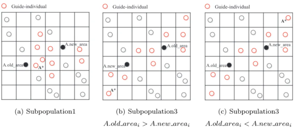
For the individualsub1 indivthat wants to go back in subpopulation1, first-ly, we need to calculate which unit domain coordinates of guide-individuals are located betweensub1 indiv.old areai and sub1indiv.new areai, and then we select the individual that is the closest tosub1 indiv.old areai. If multiple in-dividuals are in the same unit domain, the representative individual in the unit domain is selected.
For the individual sub2indiv that does not want to make any change in subpopulation2, a recombination operation is not needed.
For the individual sub3indiv that does not want to go back in subpopu-lation3: if sub3 indiv.old areai > sub3indiv.new areai, we need to calculate
which unit domain coordinates of guide-individuals are greater thansub3 indiv.old areai, and then select the individual that is the farthest to sub3 indiv.old areai. If
sub3indiv.old areai < sub3 indiv.new areai, we need to calculate which unit
domain coordinates of guide-individuals are less thansub3indiv.old areai, and then select the individual that is the farthest tosub3 indiv.old areai. Similarly, if multiple individuals are in the same unit domain, the representative individual in the unit domain is selected.
Fig. 7 is an example of recombination strategy. For individual A, the selected another parent individual for recombination is A*.
A* A.old_area A.new_area Guide-individual A* A.old_area A.new_area Guide-individual A* A.old_area A.new_area Guide-individual
(a) Subpopulation1 (b) Subpopulation3 (c) Subpopulation3 A.old areai> A.new areai A.old areai< A.new areai
Algorithm 2AdaptiveAdjustment
Require: sub1(subpopulation1),sub2(subpopulation2)
sub3(subpopulation3)
1: for allsubpopulationsub1,sub2,sub3do
2: Count the number of non-dominated individuals (num1, num2, num3) in each subpopulation and the size of each subpopulation
(sub1.size, sub2.size, sub3.size).
3: end for
4: Calculate the radio to the size of the subpopulation itself, r1 = num1/sub1.size, r2=num2/sub2.size, r3=num3/sub3.size.
5: Select the largest radiormax,max=1 or 2 or 3. 6: if i! =maxandsubi.size >10then
7: submax.size=submax.size+subi.size∗20% 8: subi.size=subi.size−subi.size∗20%
9: end if
10: Update the preset size of each subpopulation next time.
Meanwhile, in order to better solve some DMOPs with regular changes, the size of three sub-populations is adaptively adjusted. First, the combined popu-lation of the three sub-popupopu-lations is evaluated. We count the non-dominated individuals, and then compare the ratio of number of non-dominated individu-als in each population to the size of the subpopulation. For the two sub-populations with smaller ratios, when the environment changes next time, the size of two sub-populations is reduced by 20%, and no longer decreased until its size is less than 10. The size of the subpopulation with the largest ratio will increase accordingly. Algorithm 2 gives a detailed procedure of adaptive adjustment strategy.
In addition, for periodic DMOPs, we introduce the strategy of memory when the environment changes. We store the non-dominated individuals of the current population in the memory pool, non-dominated sort these stored individuals in the memory pool, and selectM sizeoptimal individuals which adapt best to the new environment. When the size of memory pool is over twice of the population
Algorithm 3DEE-DMOEA
Require: pop(current population),gmax(total number of generation)
1: Initialize a populationpop; sett:= 0; set iteration countergt:= 0.
2: Construct the dynamic environment according to Eq. (3).
3: Detect changes in the environment, if environment has not changed, turn to Step
76; else generate a new series of guide-individuals by environmental evaluation.
4: Environmental regulation, divide subpopulation.
5: Environmental guiding mechanism, recombine individuals and obtain new initial population.
6: Environmental facilitating mechanism, optimize current populationpop.
7: Ifgt > gmax, outputpopand stop; else, setgt:=gt+ 1, return to Step 2.
size, we use the principle of first in first out (FIFO) to update the memory pool, which ensures that the algorithm does not consume too much extra storage space and evaluation.
4.7. The frame of DEE-DMOEA
Now, we give the main procedure of DMOEA. The purpose of DEE-DMOEA is to accelerate the convergence speed of the population at the static optimization phase and improve the convergence and distribution of the popula-tion. Meanwhile, it is to obtain new initial population after each environmental change, so that the new population can quickly respond to changes in the dy-namic environment. The pseudo-code of DEE-DMOEA is presented in detail in Algorithm 3.
5. Test Instances and Performance Metrics
5.1. Test Instances
In this paper, a series of test problems proposed in [34] with linear or nonlin-ear correlation between design variables were selected of various DMOOP types [1] to compare the performance. Among them, F1 and F4 are from the FDA test suite [1], F2 and F3 are from the DMOP test suite [23], and F5-F10 are
newly proposed in [34]. JY1 and JY5 are newly proposed in [51]. F1-F4 are linear correlation between the decision variables, while F5-F10 are nonlinear correlation between the decision variables. Especially, F9 and F10 are more complicated problems, and it is more difficult for an algorithm to converge on them. The details of the ten problems can be found in [34].
5.2. Performance Metrics
Some metrics have been designed for dynamic optimization [45, 47, 46]. In this paper, we introduce the dynamic generational distance (DGD) [23] and inverted generational distance (DIGD) [34] metrics for DMOPs. The DGD and DIGD metrics are defined as follows:
DGD= 1 |T| P tǫT GD(P Ft, Pt), GD(P Ft, Pt) = P vǫPtd(P Ft, v) |Pt| DIGD= 1 |T| P tǫT IGD(P Ft, Pt), IGD(P Ft, Pt) = P vǫP Ftd(v, Pt) |P Ft| (8)
whereP Ftis a set of uniformly distributed Pareto optimal points in theP F at timet, andPtis the solutions obtained at timet. d(P Ft, v) =min
uǫP Ft r Pm j=1 fj(u)−fj(v) 2
is the distance betweenv andP Ft; d(v, Pt) =min uǫPt r Pm j=1 fj(v)−fj(u) 2
is the distance betweenvandPt;T is a set of discrete time points in a run and
|T|is the cardinality of T. DGD evaluates convergence of the algorithm. The lower the DGD value is, the better convergence the obtained solution set has. DIGD is a comprehensive metric to evaluate the convergence and distribution. A lower DIGD value means that solution set obtained has better convergence and distribution.
6. Experiments
In this section, DEE-DMOEA will be compared to three other algorithm-s: the dynamic cooperative-competitive evolutionary algorithm (dCOEA),
pro-posed by Goh and Tan [23], the population prediction strategy using optimiza-tion algorithm RM-MEDA [43] (PPS-RM), proposed by Zhou et al.[34], and the diversity maintenance on prediction, proposed by Ruan et al.[50]. In DEE-DMOEA, the number of unit domain on each dimension is 40; the number of guide-individual is 100; the number of selected optimal individuals from memo-ry poolM size= 5 (three objectives: 10). The population sizeN = 100 (three objectives: 200); frequency of change τT = 25; severity of change nT = 10. Other parameter settings of the three strategies use the given settings in [23] and [34].
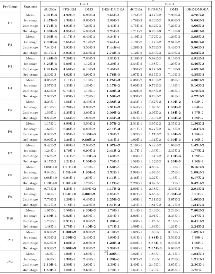
Since the DEE-DMOEA in this paper needs to consume one time of evalua-tion in generating guide-individuals and memory pool. To be fair, the algorithm iterations require removing the number of evaluations consumed at every envi-ronmental change, and reducing the corresponding number of iterations. There-fore, the frequency of change is set to beτT = 23 in DEE-DMOEA. We ran each algorithm 20 times for each test instance independently. Each simulation ran for 2500 generations (DEE-DMOEA: 2300 generations) and each strategy was tracked to 100 times of environmental changes. As the dynamic test problems introduced in Section 5 are all period, according to the parameter setting of nT, the environment will change periodically with unequal frequency ranging from 2 to 40. So, in order to discuss the performances of different strategies in each period, the result of the experiment is divided into three stages except for the first environmental change. Each stage tracks to 33 times of environmental changes and its average is taken as the result. The statistical results of DIGD and DGD over 20 runs can be found in Table 1.
6.1. Comparative Study
As can be seen in Table 1, in terms of comprehensive evaluation, DEE-DMOEA performs better than dCOEA, PPS-RM and DMS on most of the test problems; the mean DIGD in each stage is the smallest and becomes more and more stable. Especially, in the first stage, the metric values are significantly better than the other three algorithms. On F1-F4, where the decision variables
Table 1: Statistical results of DIGD and DGD metric for four algorithms
Problems Statistic DGD DIGD
dCOEA PPS-RM DMS DEE-DMOEA dCOEA PPS-RM DMS DEE-DMOEA
F1
Mean 2.01E-3 4.92E-2 6.90E-3 2.56E-3 1.75E-2 3.17E-2 7.90E-3 4.78E-3
1st stage 2.47E-3 1.38E-1 9.00E-3 2.99E-3 1.78E-2 8.26E-2 9.60E-3 5.08E-3
2nd stage 1.71E-3 4.93E-3 7.20E-3 2.43E-3 1.75E-2 6.32E-3 7.20E-3 4.66E-3
3rd stage 1.86E-3 4.85E-3 5.80E-3 2.25E-3 1.71E-2 6.28E-3 7.10E-3 4.60E-3
F2
Mean 7.95E-4 5.17E-3 9.40E-3 8.24E-4 1.19E-2 7.72E-3 1.29E-2 3.88E-3
1st stage 7.90E-4 7.65E-3 2.12E-2 9.54E-4 1.19E-2 1.17E-2 2.81E-2 3.98E-3
2nd stage 7.84E-4 3.92E-3 3.50E-3 7.44E-4 1.26E-2 5.73E-3 5.40E-3 3.86E-3
3rd stage 8.11E-4 3.93E-3 3.50E-3 7.73E-4 1.12E-2 5.66E-3 5.40E-3 3.82E-3
F3
Mean 2.48E-3 7.29E-2 7.80E-3 2.51E-3 2.16E-2 5.68E-2 9.10E-3 4.91E-3
1st stage 3.23E-3 2.09E-1 1.12E-2 3.30E-3 2.54E-2 1.58E-1 1.29E-2 5.49E-3
2nd stage 1.91E-3 4.56E-3 6.10E-3 2.46E-3 1.98E-2 6.17E-3 7.10E-3 4.89E-3
3rd stage 2.30E-3 4.62E-3 5.90E-3 1.78E-3 1.97E-2 6.15E-3 7.10E-3 4.35E-3
F4
Mean 3.05E-2 1.11E-1 1.10E-1 1.75E-2 5.38E-2 9.13E-2 1.08E-1 4.90E-2
1st stage 2.57E-2 1.33E-1 1.30E-1 2.17E-2 5.60E-2 9.76E-2 1.16E-1 5.16E-2
2nd stage 3.66E-2 9.74E-2 1.10E-1 1.60E-2 5.22E-2 8.48E-2 1.04E-1 4.78E-2
3rd stage 2.92E-2 1.03E-1 1.70E-1 1.50E-2 5.33E-2 8.78E-2 1.04E-1 4.77E-2
F5
Mean 2.23E-1 1.86E-1 2.40E-2 2.38E-2 3.33E-1 7.62E-2 1.50E-2 1.93E-2 1st stage 4.13E-1 5.20E-1 3.90E-2 3.61E-2 5.54E-1 1.92E-1 1.80E-2 2.64E-2 2nd stage 1.59E-1 2.25E-2 3.00E-2 2.09E-2 2.58E-1 2.07E-2 1.38E-2 1.77E-2 3rd stage 9.83E-2 1.56E-2 1.80E-2 1.44E-2 1.87E-1 1.59E-2 1.33E-2 1.39E-2
F6
Mean 1.15E-1 8.90E-2 3.50E-2 1.57E-2 2.51E-1 3.95E-2 2.35E-2 1.36E-2
1st stage 1.62E-1 2.36E-1 8.80E-2 2.11E-2 3.71E-1 8.77E-2 5.16E-2 1.64E-2
2nd stage 8.32E-2 1.85E-2 9.00E-3 1.38E-2 1.92E-1 1.77E-2 9.40E-3 1.28E-2 3rd stage 9.90E-2 1.26E-2 9.50E-3 1.21E-2 1.90E-1 1.31E-2 9.60E-3 1.16E-2
F7
Mean 9.42E-2 1.68E-1 2.80E-2 1.87E-2 2.19E-1 5.42E-2 1.66E-2 1.42E-2
1st stage 1.24E-1 4.79E-1 6.90E-2 2.41E-2 3.17E-1 1.36E-1 3.37E-2 1.77E-2
2nd stage 7.69E-2 1.41E-2 6.90E-3 1.50E-2 1.83E-1 1.41E-2 8.10E-3 1.29E-2 3rd stage 8.17E-2 1.21E-2 7.00E-3 1.70E-2 1.58E-1 1.26E-2 8.20E-3 1.20E-2
F8
Mean 1.08E+0 1.21E+0 1.70E-1 1.53E-1 2.58E-1 3.83E-1 1.19E-1 9.15E-2
1st stage 9.84E-1 1.55E+0 1.90E-1 2.32E-1 2.98E-1 4.64E-1 1.25E-1 1.08E-1
2nd stage 1.08E+0 9.94E-1 1.60E-1 1.11E-1 2.46E-1 3.22E-1 1.16E-1 8.17E-2
3rd stage 1.19E+0 1.10E+0 1.70E-1 1.17E-1 2.29E-1 3.62E-1 1.17E-1 8.42E-2
F9
Mean 9.76E-2 4.25E-1 5.50E-02 4.17E-2 2.00E-1 2.38E-1 3.30E-2 2.91E-2
1st stage 1.34E-1 1.04E+0 4.90E-2 8.85E-2 3.07E-1 5.65E-1 3.06E-2 5.91E-2
2nd stage 7.70E-2 1.20E-1 6.40E-2 2.25E-2 1.60E-1 7.11E-2 3.67E-2 1.60E-2
3rd stage 8.17E-2 1.18E-1 5.30E-2 1.41E-2 1.34E-1 7.81E-2 3.17E-2 1.24E-2
F10
Mean 1.97E-1 5.56E-1 8.30E-2 1.70E-1 2.14E-1 2.43E-1 2.24E-1 7.80E-2
1st stage 2.69E-1 9.02E-1 2.80E-1 3.54E-1 3.00E-1 3.91E-1 2.35E-1 1.47E-1
2nd stage 1.73E-1 3.91E-1 3.80E-2 1.20E-1 1.83E-1 1.75E-1 2.16E-1 6.41E-2
3rd stage 1.48E-1 3.75E-1 3.40E-2 3.71E-2 1.59E-1 1.64E-1 1.26E-1 2.24E-2
JY1
Mean 8.80E-2 1.00E-2 3.80E-2 4.10E-2 1.82E-1 1.86E-1 3.16E-1 1.82E-1
1st stage 9.30E-2 2.30E-2 2.40E-2 5.90E-2 5.81E-1 1.88E-2 3.50E-2 5.49E-2 2nd stage 8.50E-2 4.00E-3 3.90E-2 1.20E-2 5.80E-1 7.53E-3 2.40E-2 1.50E-2 3rd stage 8.90E-2 3.90E-3 3.80E-2 9.30E-3 5.80E-1 7.35E-3 5.60E-2 1.29E-2
JY5
Mean 1.60E-1 1.90E-1 4.80E-1 1.60E-1 1.82E-1 1.86E-1 3.16E-1 1.82E-1
1st stage 1.60E-1 1.30E-1 2.40E-1 1.20E-1 9.97E-2 1.28E-1 4.23E-1 1.21E-1 24
are linearly correlated, the mean DIGD of dCOEA is less than that of PPS-RM, but in the later two stages, PPS-RM performs better than dCOEA. On F5-F8, where the decision variables are nonlinearly correlated, dCOEA performs worse than PPS-RM, and with the environmental periodic changes and the accumulation of experience, PPS-RM will stabilize in the latter two stages and shows a gradual improved trend. On F9 and F10, which are more complicated problems, the performances of dCOEA and PPS-RM are not satisfactory. On JY1, DEE-DMOEA is the best for the mean value; PPS-RM is the best for the other stages. On JY5, DEE-DMOEA is the best for all the stages.
In terms of convergence evaluation, DEE-DMOEA shows the best perfor-mance on most test problems. On F1, F2 and F3 problems, the DGD of d-COEA is relatively average and slightly better than that of DEE-DMOEA. But overall, the metric values are similar to DEE-DMOEA. Similar to the results of comprehensive evaluation, dCOEA performs better on problems which have linear correlation between decision variables, and performs worse on problems which have nonlinear correlation between decision variables than PPS-RM.
It is not hard to explain the results. It is mainly because the environmental facilitating mechanism of DEE-DMOEA can accelerate the convergence speed of the population at the static optimization phase after environmental changes. Meanwhile, the mechanism can guide the individuals to evolve toward the do-main to be oriented, thereby improving the convergence and distribution of the population. When a change is detected, the environmental guiding mech-anism helps the population to respond quickly to new changes and generate a new initial population and accelerate the convergence of the algorithm to the new optimal solutions. dCOEA is a competitive-cooperative co-evolutionary algorithm; it generates new individuals by selecting representatives of different sub-populations and themselves to recombine and evaluate. This method can achieve good results in solving problems where the decision variables are linear-ly correlated. However, on solving problems which have nonlinear correlation between the decision variables, it is ineffective.
center at the next time by storing the population center on a continuous time series. Meanwhile, it predicts a new population distribution of the next time by recording the shape of population in the last two moments. The algorithm relies on the periodic environmental changes and accumulation of experience, so at the initial stages, the performance is poor. Along with the periodic changes, the accumulation of historical information could be sufficient to better predict the initial population. Therefore, PPS-RM will stabilize in the latter two stages.
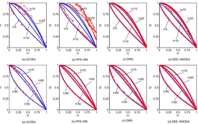
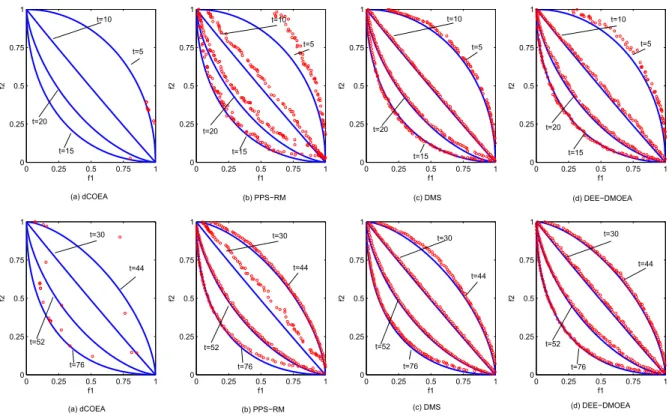
6.2. Comparison of Distribution of Final Obtained Population
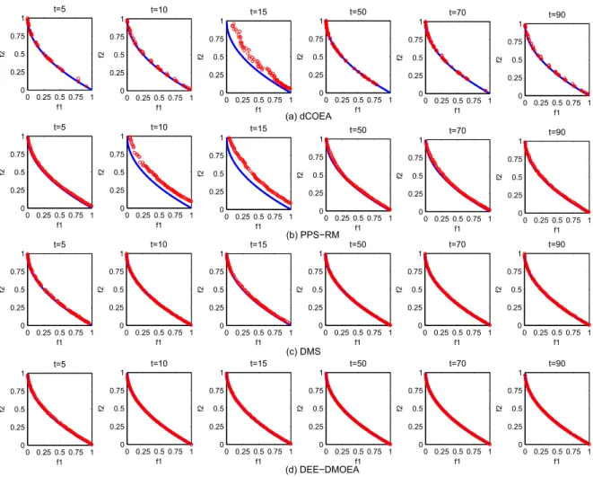
In order to visually analyze the performance of each algorithm, we choose four typical test problems, F1, F3, F6, and F9, and draw the distribution of final obtained populations of four algorithms for solving them at different time, shown in Fig. 8 to Fig. 11.
By comparison, the experimental results are similar to those in the previous section. The convergence and diversity of DEE-DMOEA are far better than dCOEA and PPS-RM at the beginning stages of environmental change, which indicates that DEE-DMOEA is able to respond to environmental changes more quickly and accurately. Furthermore, the convergence and diversity of PPS-RM is poor, indicating when the accumulation of information is insufficient, PPS-RM can not make accurate predictions. In the later stages of running, DEE-DMOEA is the same as PPS-RM, which has a better convergence and distribution, and is slightly better than PPS-RM on the nonlinear problems. Although dCOEA can obtain solutions with better convergence on the linear problems, the distribution of solutions is poor. When solving nonlinear problems, dCOEA can only obtain a few of the dominated individuals, which indicates that the algorithm is not suitable for solving such problems. As to the ability to solve the complicated problem F9, the advantage of DEE-DMOEA is more obvious. The three other algorithms can not achieve better convergence and distribution, while DEE-DMOEA can more accurately track to new optimal solutions and obtain a Pareto optimal solution set with better convergence and distribution. It indicates that DEE-DMOEA is more suitable for solving complicated nonlinear problems than
0 0.25 0.5 0.75 1 0 0.25 0.5 0.75 1 t=5 f1 f2 0 0.25 0.5 0.75 1 0 0.25 0.5 0.75 1 t=10 f1 f2 0 0.25 0.5 0.75 1 0 0.25 0.5 0.75 1 t=15 f1 f2 0 0.25 0.5 0.75 1 0 0.25 0.5 0.75 1 t=50 f1 f2 0 0.25 0.5 0.75 1 0 0.25 0.5 0.75 1 t=70 f1 f2 0 0.25 0.5 0.75 1 0 0.25 0.5 0.75 1 t=90 f1 f2 0 0.25 0.5 0.75 1 0 0.25 0.5 0.75 1 t=5 f1 f2 0 0.25 0.5 0.75 1 0 0.25 0.5 0.75 1 t=10 f1 f2 0 0.25 0.5 0.75 1 0 0.25 0.5 0.75 1 t=15 f1 f2 0 0.25 0.5 0.75 1 0 0.25 0.5 0.75 1 t=50 f1 f2 0 0.25 0.5 0.75 1 0 0.25 0.5 0.75 1 t=70 f1 f2 0 0.25 0.5 0.75 1 0 0.25 0.5 0.75 1 t=90 f1 f2 0 0.25 0.5 0.75 1 0 0.25 0.5 0.75 1 t=5 f1 f2 0 0.25 0.5 0.75 1 0 0.25 0.5 0.75 1 t=10 f1 f2 0 0.25 0.5 0.75 1 0 0.25 0.5 0.75 1 t=15 f1 f2 0 0.25 0.5 0.75 1 0 0.25 0.5 0.75 1 t=50 f1 f2 0 0.25 0.5 0.75 1 0 0.25 0.5 0.75 1 t=70 f1 f2 0 0.25 0.5 0.75 1 0 0.25 0.5 0.75 1 t=90 f1 f2 0 0.25 0.5 0.75 1 0 0.25 0.5 0.75 1 t=5 f1 f2 0 0.25 0.5 0.75 1 0 0.25 0.5 0.75 1 t=10 f1 f2 0 0.25 0.5 0.75 1 0 0.25 0.5 0.75 1 t=15 f1 f2 0 0.25 0.5 0.75 1 0 0.25 0.5 0.75 1 t=50 f1 f2 0 0.25 0.5 0.75 1 0 0.25 0.5 0.75 1 t=70 f1 f2 0 0.25 0.5 0.75 1 0 0.25 0.5 0.75 1 t=90 f1 f2 (a) dCOEA (b) PPS−RM (c) DMS (d) DEE−DMOEA
0 0.25 0.5 0.75 1 0 0.25 0.5 0.75 1 f1 f2 0 0.25 0.5 0.75 1 0 0.25 0.5 0.75 1 f1 f2 0 0.25 0.5 0.75 1 0 0.25 0.5 0.75 1 f1 f2 0 0.25 0.5 0.75 1 0 0.25 0.5 0.75 1 f1 f2 0 0.25 0.5 0.75 1 0 0.25 0.5 0.75 1 f1 f2 0 0.25 0.5 0.75 1 0 0.25 0.5 0.75 1 f1 f2 0 0.25 0.5 0.75 1 0 0.25 0.5 0.75 1 f1 f2 0 0.25 0.5 0.75 1 0 0.25 0.5 0.75 1 f1 f2 t=15 t=20 t=5 t=5 t=5 t=5 t=10 t=15 t=20 t=10 t=15 t=20 t=10 t=15 t=20 t=80 t=70 t=60 t=50 t=80 t=70 t=60 t=50 t=80 t=70 t=60 t=50 t=80 t=70 t=60 t=10 t=50 (a) dCOEA (b) PPS−RM (a) dCOEA (b) PPS−RM (c) DMS (c) DMS (d) DEE−DMOEA (d) DEE−DMOEA
0 0.25 0.5 0.75 1 0 0.25 0.5 0.75 1 f1 f2 0 0.25 0.5 0.75 1 0 0.25 0.5 0.75 1 f1 f2 0 0.25 0.5 0.75 1 0 0.25 0.5 0.75 1 f1 f2 0 0.25 0.5 0.75 1 0 0.25 0.5 0.75 1 f1 f2 0 0.25 0.5 0.75 1 0 0.25 0.5 0.75 1 f1 f2 0 0.25 0.5 0.75 1 0 0.25 0.5 0.75 1 f1 f2 0 0.25 0.5 0.75 1 0 0.25 0.5 0.75 1 f1 f2 0 0.25 0.5 0.75 1 0 0.25 0.5 0.75 1 f1 f2
(a) dCOEA (b) PPS−RM (c) DMS (d) DEE−DMOEA
(a) dCOEA (b) PPS−RM (c) DMS (d) DEE−DMOEA
t=20 t=20 t=15 t=15 t=10 t=5 t=20 t=5 t=15 t=5 t=20 t=15 t=52 t=76 t=30 t=44 t=30 t=44 t=52 t=52 t=76 t=30 t=30 t=44 t=44 t=10 t=10 t=5 t=10 t=52 t=76 t=76
0 0.25 0.5 0.75 1 0 0.25 0.5 0.75 1 f1 f2 0 0.25 0.5 0.75 1 0 0.25 0.5 0.75 1 f1 f2 0 0.25 0.5 0.75 1 0 0.25 0.5 0.75 1 f1 f2 0 0.25 0.5 0.75 1 0 0.25 0.5 0.75 1 f1 f2 0 0.25 0.5 0.75 1 0 0.25 0.5 0.75 1 f1 f2 0 0.25 0.5 0.75 1 0 0.25 0.5 0.75 1 f1 f2 0 0.25 0.5 0.75 1 0 0.25 0.5 0.75 1 f1 f2 0 0.25 0.5 0.75 1 0 0.25 0.5 0.75 1 f1 f2 t=5 t=5 t=5 t=5 t=10 t=10 t=10 t=15 t=15 t=15 t=15 t=20 t=20 t=20 t=20 t=10 t=30 t=30 t=30 t=44 t=44 t=44 t=44 t=30 t=52 t=52 t=52 t=52 t=76 t=76 t=76 t=76 (a) dCOEA (b) PPS−RM (a) dCOEA (c) DMS (c) DMS (d) DEE−DMOEA (d) DEE−DMOEA (b) PPS−RM
0 10 20 30 40 50 60 70 80 90 100 0 0.1 0.2 0.3 0.4 FDA1 Number of changes IG D DEE−DMOEA−Random DEE−DMOEA−Guide 0 10 20 30 40 50 60 70 80 90 100 0 0.5 1 1.5 F6 Number of changes IG D DEE−DMOEA−Random DEE−DMOEA−Guide
Figure 12: IGD trend comparison of DEE-dMOEA-Random and DEE-dMOEA-Guide over number of changes for 20 runs on FDA1 and F6.
the other three algorithms.
6.3. Comparison of DEE-DMOEA-Guide and DEE-DMOEA-Random
In Section 4.3 Environmental Evaluation, we generated some guide-individuals to guide evolution when evaluation was for population. For deeper observation of the role of the part, we use random individuals to replace the guide-individuals. The algorithm with random individuals is called DEE-dMOEA-Random, and the algorithm with guide-individuals is called DEE-dMOEA-Guide.
Fig. 12 shows the IGD trend comparison of DEE-dMOEA-Random and DEE-dMOEA-Guide over the number of changes for 20 runs on FDA1 and F6. On FDA1, it can be seen that the IGD graph of DEE-dMOEA-Guide is below the IGD graph of DEE-dMOEA-Random over most of the changes, espe-cially in the early stage. On F6, the comparison result of IGD trend is similar to FDA1. However, the fluctuation on F6 is larger than FDA1. Overall, the effect of DEE-dMOEA-Guide is better than DEE-dMOEA-Random.
7. Conclusions
In this paper, we have proposed a dynamic multiobjective evolutionary al-gorithm based on a dynamic environment evolutionary model (DEE-DMOEA) to solve dynamic multiobjective problems. In the proposed algorithm, we build a dynamic environment evolutionary model, which makes use of the dynamic environment to record different knowledge and information generated by pop-ulation before and after an environmental change, and in turn, the knowledge and information guide the search in the dynamic environment. The model ac-celerates the convergence speed of population at the static optimization phase and improve the convergence and distribution of the population. Furthermore, it enhances population diversity by guided method when a change is detect-ed, so that the new population can quickly respond to changes in the dynamic environment.
Compared with three other algorithms, DEE-DMOEA has shown faster re-sponse to the environmental changes than peer algorithms in solving linear or nonlinear problems, with its solution set having better convergence and diver-sity. Our future work will be designing a more accurate dynamic environment evolutionary model. Furthermore, our focus in the future will also be the ap-plications of the dynamic multiobjective evolutionary algorithms in practical problems.
Acknowledgement
This work was supported by the research projects: the National Natural Sci-ence Foundation of China under Grant Nos. 61502408 and 61673331, the Educa-tion Department Major Project of Hunan Province under Grant No. 17A212615 the CERNET Innovation Project under Grant No. NGII20150302.
References
[1] M. Farina, K. Deb, and P. Amato, “Dynamic multiobjective optimization problems: test cases, approximations, and applications,” IEEE Trans. Evol. Comput., 2004, 8(5):425-442.
[2] J. Branke, “Evolutionary optimization in dynamic environments,” Kluwer Academic Publishers, 2002.
[3] Y. Jin, and J. Branke, “Evolutionary optimization in uncertain environments-A survey,” IEEE Trans. Evol. Comput., 2005, 9(3):303-317. [4] T. T. Nguyen, S. Yang and J. Branke “Evolutionary dynamic optimization:
A survey of the state of the art,” Swarm and Evolutionary Computation, 2012, 6:1-24.
[5] M. Helbig, A. P. Engelbrecht, “Population-based metaheuristics for con-tinuous boundary-constrained dynamic multi-objective optimisation prob-lems,” Swarm and Evolutionary Computation, Vol. 14, pp. 34-46, 2014. [6] C. A. C. Coello, “20 Years of evolutionary multiobjective optimization:
what has been done and what remains to be done,” in Computational Intelligence: Principles and Practice, IEEE Computational Intelligence Society., 2006, pp. 73-88.
[7] C. A. C. Coello, D. A. van Veldhuizen, and G. B. Lamont, “Evolutionary al-gorithms for solving multiobjective problems,” New York: Springer-Verlag, 2007.
[8] S. Yang, M. Li, X. Liu, and J. Zheng, “A grid-based evolutionary algorithm for many-objective optimization,” IEEE Trans. Evol. Comput., vol. 17, no. 5, pp. 721-736, Oct. 2013.
[9] M. Li, S. Yang, and X. Liu, “Shift-Based density estimation for pareto-based algorithms in many-objective optimization,” IEEE Trans. Evol. Comput., 18(3): 348-365, June 2014.
[10] Z. Avdagic, S. Konjicija, and S. Omanovic, “Evolutionary approach to solving non-stationary dynamic multiobjective problems,” Foundations of Computational Intelligence Volume 3, ser. Studies in Computational Intel-ligence, A. Abraham, A.-E. Hassanien, P. Siarry, and A. Engelbrecht, Eds. Springer Berlin/Heidelberg, 2009, vol. 203, pp. 267-289.
[11] R. Shang, L. Jiao, Y. Ren, L. Li, and L. Wang, “Quantum immune clonal coevolutionary algorithm for dynamic multiobjective optimization,” Soft Computing, 2013, 1-14.
[12] M. Greeff and A. P. Engelbrecht, “Solving dynamic multiobjective problems with vector evaluated particle swarm optimization,” in Proc. IEEE Congr. Evol. Comput., 2008, 2922-2929.
[13] L. Huang, H. Suh and A. Abraham, “Dynamic multiobjective optimization based on membrane computing for control of time-varying unstable plants,” Information Sciences, 2011. 181:2370-2391.
[14] A. Isaacs, V. Puttige, T. Ray, W. Smith, and S. Anavatti, “Development of a memetic algorithm for dynamic multiobjective optimization and its applications for online neural network modeling of UAVs,” in International Joint Conference on Neural Networks (IJCNN 2008), 2008, pp. 548-554. [15] R. Liu, W. Zhang, L. Jiao, F. Liu and J. Ma, “A sphere-dominance based
preference immune-inspired algorithm for dynamic multiobjective opti-mization,” in Genetic and Evolutionary Computation Conference (GECCO 2010), 2011, 423-430.
[16] J. Wei and Y. Wang, “Hyper rectangle search based particle swarm algo-rithm for dynamic constrained multiobjective optimization problems,” in Proc. IEEE Congr. Evol. Comput (CEC2012)., 2012, 259-266.
[17] C. Liu and Y. Wang, “Multiobjective evolutionary algorithm for dy-namic nonlinear constrained optimization problems,” Journal of Systems Engineering and Electronics, vol. 20, no. 1, pp. 204-210, 2009.
[18] C. Liu and Y. Wang, “New evolutionary algorithm for dynamic multiob-jective optimization problems,” in Evolutionary Computation: Theory and Algorithms, vol. LNCS 4221, 2006, pp. 889-892.
[19] C. R. B. Azevedo and A. F. R. Araujo, “Generalized immigration schemes for dynamic evolutionary multiobjective optimization,” in Proc. IEEE Congr. Evol. Comput., 2011. 2033-2040.
[20] A. D. Manriquez, G. T. Pulido and J. G. R. Torres, “Handling dynamic multiobjective problems with particle swarm optimization,” in 2nd International Conference on Agents and Artificial Intelligence (ICAART2010), 2010. 337-342.
[21] M. Camara, J. Ortega and F. de Toro, “Approaching dynamic multiob-jective optimization problems by using parallel evolutionary algorithms,” Advances in multiobjective Nature Inspired Computing, 2010. 272:63-86. [22] B. Zheng, “A new dynamic multiobjective optimization evolutionary
algo-rithm,” in Third International Conference on Natural Computation (ICNC 2007), 2007, pp. 565-570.
[23] C. K. Goh and K. C. Tan, “A competitive-cooperative coevolutionary paradigm for dynamic multiobjective optimization,” IEEE Trans. Evol. Comput., 2009. 13:103-127.
[24] C. K. Goh, and K. C. Tan, “Evolutionary multiobjective Optimization in Uncertain Environments: Issues and Algorithms,” springer-Verlag, Berlin, 2009.
[25] K. Deb, U. V. Rao, and S. Karthik, “Dynamic multiobjective optimiza-tion and decision-making using modified NSGA-II- a case study on hydro-thermal power scheduling,” in Evolutionary Multi-Criterion Optimization (EMO 2007), 2007, LNCS 4403, pp. 803-817.
[26] Z. Zhang, “Multiobjective optimization immune algorithm in dynamic environments and its application to greenhouse control,” Applied Soft Computing, vol. 8, no. 2, pp. 959-971, 2008.
[27] X. Yao, Y. Liu, and G. Lin, “Evolutionary programming made faster,” IEEE Trans. Evol. Comput., 3(2): 82-102, 1999.
[28] Y. Wang and B. Li, “Investigation of memory-based multiobjective opti-mization evolutionary algorithm in dynamic environment,” in Proc. IEEE Congr. Evol. Comput., 2009, 630-637.
[29] A. Isaacs, V. Puttige, T. Ray, W. Smith, and S. Anavatti, “Development of a memetic algorithm for dynamic multiobjective optimization and its applications for online neural network modeling of UAVs,” in International Joint Conference on Neural Networks (IJCNN 2008), 2008, pp. 548-554. [30] S. Guan, Q. Chen, and W. Mo, “Evolving dynamic multiobjective
optimiza-tion problems with objective replacement,” Artificial Intelligence Review, vol. 23, pp. 267-293, 2005.
[31] I. Hatzakis, and D. Wallace, “Dynamic multiobjective optimization with evolutionary algorithms: A forward-looking approach,” in Genetic and Evolutionary Computation Conference (GECCO 2006), 2006, 1201-1208. [32] I. Hatzakis, and D. Wallace, “Topology of anticipatory populations for
evolutionary dynamic multiobjective optimization,” in 11th AIAA/ISSMO Multidisciplinary Analysis and Optimization Conference, 2006.
[33] A. Zhou, Y. Jin, Q. Zhang, B. Sendhoff and E. Tsang, “Prediction-based population re-initialization for evolutionary dynamic multiobjective op-timization,” in Evolutionary Multi-Criterion Optimization (EMO 2007), 2007.832-846.
[34] A. Zhou, Y. Jin, and Q. Zhang, “A population prediction strategy for evolutionary dynamic multiobjective optimization,” IEEE Transactions on Cybernetics, 2013.
[35] Y. Ma, R. Liu, and R. Shang, “A hybrid dynamic multiobjective immune optimization algorithm using prediction strategy and improved differential evolution crossover operator,” Neural Information Processing, 2011, vol. L-NCS 7063, pp. 435-444.
[36] Y. Wang and B. Li, “Multi-strategy ensemble evolutionary algorithm for dynamic multiobjective optimization,” Memetic Computing, vol. 2, pp. 3-24, 2009.
[37] T. M. Blackwell and P. J. Bentley, “Dynamic search with charged swarm-s,” in Genetic and Evolutionary Computation Conference (GECCO 2002), 2002.19-26.
[38] K. Deb, “Multi-Objective Optimization using Evolutionary Algorithms,” John Wiley & Sons, UK, Chichester, 2001.
[39] K. Deb, A. Sinha, and S. Kukkonen, “Multi-Objective Test Problems, Linkages, and Evolutionary Methodologies,” in Genetic and Evolutionary Computation Conference (GECCO 2006), 2006: 1141-1148.
[40] P. Borges, and M. Hansen, “A basis for future successes in multiobjective combinatorial optimization,” Technical Report IMM-REP-1998-8, Institute of Mathematical Modelling, Technical University of Denmark, March 1998. [41] M. Helbig and A. P. Engelbrecht, “Archive management for dynamic mul-tiobjective optimisation problems using vector evaluated particle swarm optimization,” in Proc. IEEE Congr. Evol. Comput (CEC2011), 2011, p-p. 2047-2054.
[42] W. T. Koo, C. K. Goh and K. C. Tan, “A predictive gradient strategy for multiobjective evolutionary algorithms in a fast changing environment,” Memetic Computing, vol. 2, pp. 87-110, 2009.
[43] Q. Zhang, A. Zhou and Y. Jin, “RM-MEDA: A regularity model based multiobjective estimation of distribution algorithm,” IEEE Trans. Evol. Comput., 2008, 12(1): 41-63.
[44] K. Deb, A. Pratap, S. Agarwal, and T. Meyarivan, “A fast and elitist multiobjective genetic algorithm: NSGA-II,” IEEE Trans. Evol. Comput., vol. 6, no. 2, pp. 182-197, 2002.
[45] M. Camara, J. Ortega, and F. de Toro, “Performance measures for dynamic multiobjective optimization,” in Bio-Inspired Systems: Computational and Ambient Intelligence. Springer, 2009. 5517:760-767.
[46] E. Tantar, A. A. Tantar and P. Bouvry, “On dynamic multiobjective opti-mization classification and performance measures,” in Proc. IEEE Congr. Evol. Comput (CEC2011)., 2011, 2759-2766.
[47] M. Helbig and A. Engelbrecht, “Issues with performance measures for dynamic multiobjective optimization,” IEEE Symposium Series on Computational Intelligence, Singapore, April 2013, pp. 17-24.
[48] Z. Peng, J. Zheng, J. Zou, and M. Liu, “Novel prediction and memo-ry strategies for dynamic multiobjective optimization,” Soft Computing, vol. 19, no. 9, pp. 2633–2653, 2015.
[49] A. Zhou, Y. Jin, and Q. Zhang, “A population prediction strategy for evo-lutionary dynamic multiobjective optimization,” IEEE Trans. on Cybern., vol. 44, no. 1, pp. 40–53, 2013.
[50] R. Gan, G. Yu, J. Zheng, J. Zou, and S. Yang. The effect of diversity main-tenance on prediction in dynamic multi-objective optimization. Applied Soft Computing, 58: 631-647, 2017.
[51] S. Jiang and S. Yang, ”Evolutionary dynamic multiobjective optimization: Benchmarks and algorithm comparisons”. IEEE Trans. on Cybern., vol. 47, no. 1, pp. 198-211, January 2017.