Contents lists available atScienceDirect
International Journal of Approximate Reasoning
j o u r n a l h o m e p a g e :w w w . e l s e v i e r . c o m / l o c a t e / i j a rMulti-dimensional classification with Bayesian networks
C. Bielza
a, G. Li
b, P. Larrañaga
a,∗aComputational Intelligence Group, Departamento de Inteligencia Artificial, Universidad Politécnica de Madrid, Boadilla del Monte, 28660 Madrid, Spain bRega Institute and University Hospitals, Katholieke Universiteit Leuven, B-3000 Leuven, Belgium
A R T I C L E I N F O A B S T R A C T Article history:
Received 30 July 2010 Revised 2 December 2010 Accepted 21 January 2011 Available online 16 February 2011
Keywords:
Multi-dimensional outputs Bayesian network classifiers Learning from data MPE
Multi-label classification
Multi-dimensional classification aims at finding a function that assigns a vector of class values to a given vector of features. In this paper, this problem is tackled by a general family of models, called multi-dimensional Bayesian network classifiers (MBCs). This probabilistic graphical model organizes class and feature variables as three different subgraphs: class subgraph, feature subgraph, and bridge (from class to features) subgraph. Under the standard 0–1 loss function, the most probable explanation (MPE) must be computed, for which we provide theoretical results in both general MBCs and in MBCs decomposable into maximal connected components. Moreover, when computing the MPE, the vector of class values is covered by following a special ordering (gray code). Under other loss functions defined in accordance with a decomposable structure, we derive theoretical results on how to minimize the expected loss. Besides these inference issues, the paper presents flexible algorithms for learning MBC structures from data based on filter, wrapper and hybrid approaches. The cardinality of the search space is also given. New performance evaluation metrics adapted from the single-class setting are introduced. Experimental results with three benchmark data sets are encouraging, and they outperform state-of-the-art algorithms for multi-label classification.
© 2011 Elsevier Inc. All rights reserved.
1. Introduction
In this paper we are interested in classification problems where there are multiple class variablesC1
, . . . ,
Cd. Thereforethemulti-dimensional classificationproblem consists of finding a functionhthat assigns to each instance given by a vector ofmfeaturesx
=
(
x1, . . . ,
xm)
a vector ofdclass valuesc=
(
c1, . . . ,
cd)
:h
:
ΩX1× · · · ×
ΩXm→
ΩC1× · · · ×
ΩCd(
x1, . . . ,
xm)
→
(
c1, . . . ,
cd)
We assume thatCiis a discrete variable, for alli
=
1, . . . ,
d, withΩCidenoting its sample space andI=
ΩC1×· · ·×
ΩCd,the space of joint configurations of the class variables. Analogously,ΩXjis the sample space of the discrete feature variable
Xj, for allj
=
1, . . . ,
m.∗Corresponding author. Tel.: +34 91 3367443; fax: +34 91 3524819.
E-mail addresses:[email protected] (C. Bielza), [email protected] (G. Li), [email protected] (P. Larrañaga). 0888-613X/$ - see front matter © 2011 Elsevier Inc. All rights reserved.
Many application domains include multi-dimensional classification problems: a text document or a semantic scene can be assigned to multiple topics, a gene can have multiple biological functions, a patient may suffer from multiple diseases, a patient may become resistant to multiple drugs for HIV treatment, a physical device can break down due to multiple components failing, etc.
Multi-dimensional classification is a more difficult problem than the single-class case. The main problem is that there
is a large number of possible class label combinations,
|
I|
, and a corresponding sparseness of available data. In a typicalscenario where an instancexis assigned to the most likely combination of classes (0–1 loss function), the aim is to compute
arg maxc1,...,cdp
(
C1=
c1, . . . ,
Cd=
cd|
x).
It holds thatp(
C1=
c1, . . . ,
Cd=
cd|
x)
∝
p(
C1=
c1, . . . ,
Cd=
cd,
x)
,which requires
|
I| · |
ΩX1× · · · ×
ΩXm|
parameters to be assigned. In the single-class case,|
I|
is just|
ΩC|
rather than|
ΩC1× · · · ×
ΩCd|
. Besides it having a high cardinality, it is also hard to estimate the required parameters from a (sparse)data set in thisd-dimensional space
|
I|
. The factorization of this joint probability distribution when using a Bayesian network(BN) can somehow reduce the number of parameters required and will be our starting point.
Standard (one-class) BN classifiers cannot be straightforwardly applied to this multi-dimensional setting. On the one hand, the problem could be transformed into a single-class problem if a compound class variable modeling all possible combinations of classes is constructed. However, this class variable would have too many values, and even worse, the model would not capture the structure of the classification problem (dependencies among class variables and also among class variables and features). On the other hand, we could approach the multi-dimensional problem by constructing one independent classifier for each class variable. However, this would not capture the interactions among class variables, and the
most likely class label for each independent classifier – marginal classifications – after being assembled as ad-dimensional
vector, might not coincide with the most likely vector of class labels of the observed data.
As we will show below, the few proposals found in the literature on multi-dimensional BN classifiers (MBCs) are limited. In this paper, we propose a comprehensive theory of MBCs, including their extended definition, learning from data algo-rithms that cover all the possibilities (wrapper, filter and hybrid score + search strategies), and results on how to perform total abduction for the exact inference of the most probable explanation (MPE). MPE computation is the main aim in 0–1 loss function classification problems but involves a high computational cost in the multi-dimensional setting. Several contribu-tions are designed here to reduce this computational load: the introduction of special decomposed MBCs, their extension to non 0–1 loss function problems that respect this decomposition, and a particular and favorable way of enumerating all the
(
c1, . . . ,
cd)
configurations instead of using a brute-force approach.The paper is organized as follows: Section 2 defines MBCs. Section 3 covers different contributions for the MPE com-putation and introduces a restricted structure of decomposable MBCs where MPE is easier to compute. Section 4 extends these ideas to compute the Bayes decision rule with certain loss functions that we call additive CB-decomposable loss func-tions. Section 5 presents performance measures suitable for evaluating MBCs. Section 6 describes wrapper, filter and hybrid algorithms to learn MBCs from data. It also provides the cardinality of the MBC structure space where these algorithms search for. Section 7 shows experimental results on MPE with simulated MBCs. Section 8 contains experimental results with three benchmark data sets. Section 9 reviews the work related to multi-dimensional classification, with special emphasis on papers using (simpler) MBCs. Finally, Section 10 sums up the paper with some conclusions.
2. Multi-dimensional Bayesian network classifiers
A Bayesian network over a finite setV
= {
Z1, . . . ,
Zn}
,n≥
1, of discrete random variables is a pairB=
(G,
Θ)
,whereG is an acyclic directed graph whose vertices correspond to the random variables andΘ is a set of parameters
θ
z|pa(z)=
p(
z|
pa(
z))
, wherepa(
z)
is a value of the set of variablesPa(
Z)
, parents of theZvariable in the graphical structureG[42,36].Bdefines a joint probability distributionpBoverVgiven by
pB
(
z1, . . . ,
zn)
=
n i=1p
(
zi|
pa(
zi)).
(1)Amulti-dimensional Bayesian network classifieris a Bayesian network specially designed to solve classification problems including multiple class variables in which instances described by a number of features have to be assigned to a combination of classes.
Definition 1(Multi-dimensional Bayesian network classifier). In anMBCdenoted byB
=
(G,
Θ)
, the graphG=
(V,
A)hasthe setVof vertices partitioned into two setsVC
= {
C1, . . . ,
Cd}
,d≥
1, of class variables andVX= {
X1, . . . ,
Xm}
,m≥
1,of feature variables
(
d+
m=
n)
.Galso has the setAof arcs partitioned into three sets,AC,AX,ACX, such that:•
AC⊆
VC×
VCis composed of the arcs between the class variables having a subgraphGC=
(V
C,
AC)
–class subgraph– ofGinduced byVC.
•
AX⊆
VX×
VX is composed of the arcs between the feature variables having a subgraphGX=
(V
X,
AX)
–featureFig. 1. An example of an MBC structure with its three subgraphs.
Fig. 2. Examples of structures belonging to different families of MBCs. (a)Empty–emptyMBC; (b)Tree–treeMBC; (c)Polytree–DAGMBC.
•
ACX⊆
VC×VXis composed of the arcs from the class variables to the feature variables having a subgraphGCX=
(V,
ACX)
–bridge subgraph– ofGconnecting class and feature variables.
This definition extends that in van der Gaag and de Waal [70], which requires two additional conditions (see Section 6.4).
Fig.1shows an example of an MBC structure and its different subgraphs.
Note that different graphical structures for the class and feature subgraphs may give rise to different families of MBCs. In general, class and feature subgraphs may be: empty, directed trees, forest of trees, polytrees, and general directed
acyclic graphs (DAG). The different families of MBCs will be denoted asclass subgraph structure-feature subgraph
structureMBC, where the possible structures are the above five. Thus, if both the class and feature subgraphs are directed
trees, then this subfamily is atree–treeMBC. Other examples are shown in Fig.2.
Note that the well-known Bayesian classifiers: naïve Bayes [40], selective naïve Bayes [37], tree-augmented naïve Bayes
[24], selective tree-augmented naïve Bayes [3] andk-dependence Bayesian classifiers [53] are special cases of MBCs where
d
=
1. Several MBC structures have been used in the literature:tree–treeMBC [70],polytree–polytreeMBC [15] anda specialDAG–DAGMBC [51].
The following theorem extends the well-known result that states that given a 0–1 loss function in a (one-dimensional) classification problem, the Bayes decision rule is to select the class label that maximizes the posterior probability of the class variable given the features. This supports the use of the percentage of correctly classified instances (or classifier accuracy) as a performance measure. In Section 5 we extend the definition of accuracy to our multi-dimensional setting.
Theorem 1. Let
λ(
c,
c)
be a 0–1 loss function that assigns a unit loss to any error, i.e. wheneverc=
c, wherec is the d-dimensional vector of class values output by a model andccontains the true class value and assigns no loss to a correct classification, i.e. whenc=
c.Let R
(
c|
x)
=
|I|j=1
λ(
c,
cj)
p(
cj|
x)
be the expected loss or conditional risk, wherex=
(
x1, . . . ,
xm)
is a vector of featurevalues and p
(
cj|
x)
is the joint posterior probability, provided by a model, of the vector of the class valuecjgiven the observationx.Then the Bayes decision rule that minimizes the expected loss R
(
c|
x)
is equivalent to selecting thec that maximizes the posterior probability p(
c|
x)
, that is,min
c R
(
c|
x)
⇔
maxc p
(
c|
x)
Proof. The proof is straightforward and analogous to the single-class variable case [22] usingC
=
(
C1, . . . ,
Cd)
as the(d-dimensional) class variable, i.e.
R
(
c|
x)
=
|I| j=1λ(
c,
cj)
p(
cj|
x)
=
cj=c p(
cj|
x)
=
1−
p(
c|
x).
Fig. 3. An example of MBC structure.
Therefore, the multi-dimensional classification problem with a 0–1 loss is equivalent to computing a type of maximum
a posteriori (MAP), known asmost probable explanation(MPE), also called total abduction [42]. This has been shown to be a
NP-hard problem for Bayesian networks [56]. Approximating the MPE problem is also NP-hard [1].
However, the special structure that defines the MBC will alleviate somewhat MPE computation under certain circum-stances, as shown in the next section.
3. Theoretical results on MPE
The NP-hardness of MPE computation in general Bayesian networks has led to the design of both exact and approximate
algorithms. Exact algorithms include approaches using junction trees [13], variable elimination [38,17], and
branch-and-bound search [34,39]. Approximate algorithms cover the use of genetic algorithms [26,52], stochastic local search algorithms
[33,31], the so-called mini-bucket approach based on variable elimination [18], best-first search [57] and linear programming
[54].
MPE computation when havingdclass variables increases the number of possible configurations exponentially, i.e. given
evidencexwe have to get
c∗
=
(
c1∗, . . . ,
c∗d)
=
arg maxc1,...,cdp
(
C1=
c1, . . . ,
Cd=
cd|
x).
(2) De Waal and van der Gaag (2007) show that the classification problem can be solved in polynomial time if the feature subgraph has bounded treewidth and the number of class variables is restricted (see their Theorem 1). This implies that the connectivity of the class subgraph is irrelevant for the feasibility of classification.This section reports two major contributions. On the one hand, thanks to the specific structure of MBCs and a special
way (gray code) of moving within theIspace of joint configurations of the class variables, we will be able, despite this high
complexity, to reduce the computations performed to obtain the posterior probabilityp
(
C1=
c1, . . . ,
Cd=
cd|
x)
and finallyget the MPE. This will be feasible for a small numberdof classes, since gray codes are helpful for exhaustively enumerating
theIspace. An upper bound for the savings achieved with respect to a brute-force approach is also provided. On the other
hand, when the graph union of class and bridge subgraphs of an MBC structure is decomposed into a number,r, of connected
subgraphs, we prove that the maximization problem for computing the MPE can be transformed intormaximization
problems operating in lower dimensional spaces. These simpler structures will be called class-bridge decomposable MBCs. Analogous results with gray codes in this case are also presented.
The main motivation for trying to enumerate theIspace lies in the similarity between the posterior probability of two
configurations that have the same class values in all components but one. This is shown in Example 1.
Example 1. Given the MBC structure of Fig.3, where all variables are assumed to be binary (0/1) andx
=
(
x1,
x2,
x3,
x4)
,the posterior probabilities of configurations
(
0,
0,
0)
and(
1,
0,
0)
for(
C1,
C2,
C3)
satisfy:p
((
0,
0,
0)
|
x)
p((
1,
0,
0)
|
x)
=
p(
0,
0,
0,
x)
p(
1,
0,
0,
x)
=
p(
C1=
0|
C2=
0)
p(
C2=
0)
p(
C3=
0|
C2=
0)
p(
X1=
x1|
C1=
0,
C2=
0)
p(
C1=
1|
C2=
0)
p(
C2=
0)
p(
C3=
0|
C2=
0)
p(
X1=
x1|
C1=
1,
C2=
0)
·
p(
X2=
x2|
C1=
0,
C2=
0,
C3=
0)
p(
X3=
x3|
C3=
0,
X1=
x1)
p(
X2=
x2|
C1=
1,
C2=
0,
C3=
0)
p(
X3=
x3|
C3=
0,
X1=
x1)
·
p(
X4=
x4|
C2=
0,
C3=
0,
X1=
x1)
p(
X4=
x4|
C2=
0,
C3=
0,
X1=
x1)
=
p(
C1=
0|
C2=
0)
p(
X1=
x1|
C1=
0,
C2=
0)
p(
X2=
x2|
C1=
0,
C2=
0,
C3=
0)
p(
C1=
1|
C2=
0)
p(
X1=
x1|
C1=
1,
C2=
0)
p(
X2=
x2|
C1=
1,
C2=
0,
C3=
0)
This may be generalized in the following proposition.Fig. 4.(3,3,2;3)-gray code.
Proposition 1. Given an MBC and an instantiation of all the feature variablesx
=
(
x1, . . . ,
xm)
, then the ratio of posteriordistributions of two d-dimensional class configurationsc
=
(
c1, . . . ,
cd)
andc=
(
c1, . . . ,
cd)
is given byp
(
c|
x)
p(
c|
x)
=
Ci∈Wp(
Ci=
ci|
pa(
ci))
Ci∈Wp(
Ci=
ci|
pa(
ci))
·
Xj∈Ch(W)p(
Xj=
xj|
pa(
xj))
Xj∈Ch(W)p(
Xj=
xj|
pa(
xj))
,
whereW
= {
Ci∈
VC| ∃!
l∈ {
1, . . . ,
d}
,
cl=
cl}
,pa(
xj)
denotes the configuration ofPa(
Xj)
compatible withxandc, andCh
(W
)
denotes the feature variables that are children of variables in setW.Proof. In the numerator, p
(
c|
x)
=
1 p(
x)
Ci∈W p(
Ci=
ci|
pa(
ci))
Ci∈/W p(
Ci=
ci|
pa(
ci))
Xj∈Ch(W) p(
Xj=
xj|
pa(
xj))
Xj∈/Ch(W) p(
Xj=
xj|
pa(
xj))
In the denominator, the factorization forp
(
c|
x)
is analogous and its first, third, and fifth factors coincide with those inp
(
c|
x)
. This leads directly to the final result.Corollary 1. In the above situation, wherecandcnow differ by only one component l, i.e. ci
=
ci∀
i=
l and cl=
cl, thenp
(
c|
x)
p(
c|
x)
=
p(
Cl=
cl|
pa(
cl))
p(
Cl=
cl|
pa(
cl))
·
Xj∈Ch(Cl)p(
Xj=
xj|
pa(
xj))
Xj∈Ch(Cl)p(
Xj=
xj|
pa(
xj))
.
These configurationscandcdiffering by one component (as in Example 1) provide more savings than in the general
case of Proposition1. For simplicity’s sake, we can chooseclandclsuch that
|
cl−
cl| =
1. In this case, an adaptation of thegray code introduced by Guan [28] is proposed for enumerating all the
(
c1, . . . ,
cd)
configurations in a special order. Guan’s(
n;
k)
-gray code is a special sequence enumerating all elements in(
Zn)
k, that is, vectors ofkcomponents each taking valuesin the space
{
0,
1, . . . ,
n−
1}
. Therefore, components are restricted to being in the same range. We, however, extend graycodes to different rangesri,i
=
1, . . . ,
d, having(
r1, . . . ,
rd;
d)
-gray codes.Definition 2(
(
r1, . . . ,
rd;
d)
-gray code). Given a vector(
C1, . . . ,
Cd)
with each componentCitaking values in{
0,
1, . . . ,
ri−
1}
,i=
1, . . . ,
d, an(
r1, . . . ,
rd;
d)
-gray codeis a sequence that enumerates all the configurations(
c1, . . . ,
cd)
such thateach pair of adjacent configurations differs by only one component and the difference is either 1 or
−
1.Example 2. Fig.4shows the sequence of configurations for a
(
3,
3,
2;
3)
-gray code, i.e. triplets where the first component takes values in{
0,
1,
2}
, the second in{
0,
1,
2}
and the third in{
0,
1}
.In this example, ifSidenotes the number of changes in theith component to cover the whole gray code, thenS3
=
1,
S2=
4
,
S1=
12 (see the boxes in Fig.4).Proposition 2. In the
(
r1, . . . ,
rd;
d)
-gray code, the number of changes, Si, in the ith component, is given by Si=
⎧ ⎪ ⎪ ⎨ ⎪ ⎪ ⎩ d j=i rj−
d j=i+1 rj,
1≤
i≤
d−
1 rd−
1,
i=
d Moreover,di=1Si=
dj=1rj−
1.Proof. Fori
=
d,
Sd=
rd−
1 since the last component is the one is moved least by gray coding. For 1≤
i≤
d−
1,Si
=
rd·
rd−1· · ·
ri+1·
(
ri−
1)
, since theith component hasri−
1 changes for each partial configuration of fixed values incomponentsi
+
1, . . . ,
d, which arerd·
rd−1· · ·
ri+1. Also, d i=1 Si=
d−1 i=1 ⎛ ⎝d j=i rj−
d j=i+1 rj ⎞ ⎠+
rd−
1=
(
r1· · ·
rd)
−
(
r2· · ·
rd)
+
(
r2· · ·
rd)
−
(
r3· · ·
rd)
+ · · · +
(
rd−1·
rd)
−
rd+
rd−
1=
r1· · ·
rd−
1.
Computations to obtain MPE in MBCs are reduced by using these gray codes. The next theorem shows the savings and an upper bound when comparing the number of factors needed in the posterior probability computations with gray codes,
FGC, and with brute-force,FBF.
Theorem 2. Given an MBC with m feature variables and d class variables, whereIis the space of joint configurations of the class variables, then the number of factors needed in the posterior probability computations with gray codes, FGC, and with brute-force,
FBF, satisfy: (i) FGC
=
m+
d+
di=1SiHi (ii) FGC FBF<
1 |I|+
HmMax+d,where Hi
=
1+
hi, hibeing the number of children (in the MBC) of the class variable that changes the ith in the gray code, andHMax
=
max1≤i≤dHi. Proof. (i)FGC=
m+
d+
d
i=1SiHi, sincem
+
dcorresponds to the number of factors (without savings) for calculating theposterior probability for the first configuration where the gray code starts from, and, using Corollary1, each configuration
that changes itsith class variable in the gray code requires 1
+
hi=
Hinew factors. Taking into account that the numberof changes in theith class variable along the gray code sequence isSi, the second term,di=1SiHi, gives the total number of
factors required by all the configurations except the first one.
(ii) Obviously,FBF
=
(
m+
d)
|
I|
. Also,FGC
=
m+
d+
d i=1 SiHi≤
m+
d+
HMax d i=1 Si=
m+
d+
HMax(
|
I| −
1),
sincedi=1Si
= |
I| −
1 is the total number of changes in the gray code. Therefore,FGC FBF
≤
m+
d+
HMax(
|
I| −
1)
(
m+
d)
|
I|
<
1|
I|
+
HMax m+
d.
Example 1(continued).Given the MBC structure of Fig.3, where variablesC1andC2now take three possible values andC3
is still binary, we have thatd
=
3,
m=
4,
HMax=
4,
|
I| =
18.Thus,
FGC
FBF
=
63126
,
and the upper bound isFGC
FBF
<
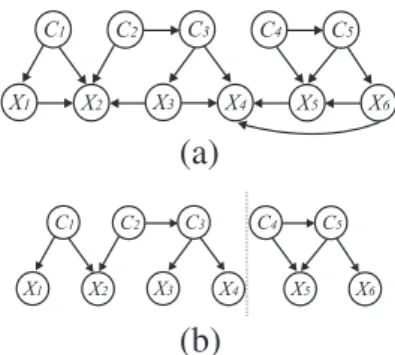
79Fig. 5. (a) A CB-decomposable MBC. (b) Its two maximal connected components.
Therefore, with gray codes the number of factors is reduced by half (63 against 126), while the upper bound is a little bit higher.
Definition 3(CB-decomposable MBC). Suppose we have an MBC whereGC andGCX are its associated class and bridge
subgraphs respectively. We say that the MBC isclass-bridge decomposable(CB-decomposable for short) if:
(1) GC
∪
GCX can be decomposed asGC∪
GCX=
ri=1(G
Ci∪
G(CX)i)
, whereGCi∪
G(CX)i, withi=
1, . . . ,
r, are itsrmaximal connected components,1 and
(2) Ch
(V
Ci)
∩
Ch(V
Cj)
=
∅
, withi,
j=
1, . . . ,
randi=
j, whereCh(V
Ci)
denotes the children of all the variables inVCi,the subset of class variables inGCi(non-shared children property).
Example 3.Let us take the MBC structure shown in Fig.5(a). It is CB-decomposable withr
=
2, as shown in Fig.5(b). Thesubgraph to the left of the dashed vertical line isGC1
∪
G(CX)1, i.e. the first maximal connected component. Analogously,GC2
∪
G(CX)2 to the right-hand side is the second maximal connected component. That is,VC1= {
C1,
C2,
C3}
,
VC2=
{
C4,
C5}
,
Ch(V
C1)
= {
X1,
X2,
X3,
X4}
andCh(V
C2)
= {
X5,
X6}
. Note thatCh(
{
C1,
C2,
C3}
)
∩
Ch(
{
C4,
C5}
)
=
∅
as required.Theorem 3. Given a CB-decomposable MBC whereIi
=
C∈VCiΩCrepresents the sample space associated withVCi, then max c1,...,cdp(
C1=
c1, . . . ,
Cd=
cd|
X1=
x1, . . . ,
Xm=
xm)
∝
r i=1 max c↓VCi∈Ii C∈VCi p(
c|
pa(
c))
X∈Ch(VCi) p(
x|
paVC(
x),
paVX(
x)),
(3)wherec↓VCirepresents the projection of vectorcto the coordinates found inV Ci.
Proof. By using firstly the factorization given in (1) and then the grouping of all the variables according to the CB-decomposable MBC assumption, we have that
p
(
C1=
c1, . . . ,
Cd=
cd|
X1=
x1, . . . ,
Xm=
xm)
∝
C∈VC p(
c|
pa(
c))
X∈VX p(
x|
paVC(
x),
paVX(
x))
=
r i=1 C∈VCi p(
c|
pa(
c))
X∈Ch(VCi) p(
x|
paVC(
x),
paVX(
x)).
Maximizing the last expression with respect to all the class variables amounts to maximizing over the identified class variables of the maximal connected components. The new maximization problems are carried out on lower dimensional subspaces than originally, thereby reducing the computational cost. Note that the feature subgraph structure is irrelevant
in this process.
1
Givenx, each expression to be maximized in Eq. (3) will be denoted as
φ
ix(
c↓VCi)
, i.e.φ
x i(
c↓VCi)
=
C∈VCi p(
c|
pa(
c))
·
X∈Ch(VCi) p(
x|
paVC(
x),
paVX(
x))
It holds thatφ
ix(
c↓VCi)
∝
p(
C↓VCi=
c↓VCi|
x).
Example 3(continued).For the CB-decomposable MBC in Fig.5(a), we have that
max c1,...,c5p
(
C1=
c1, . . . ,
C5=
c5|
X1=
x1, . . . ,
X6=
x6)
∝
max c1,...,c5p(
c1)
p(
c2)
p(
c3|
c2)
p(
c4)
p(
c5|
c4)
p(
x1|
c1)
p(
x2|
c1,
c2,
x1,
x3)
·
p(
x3|
c3)
p(
x4|
c3,
x3,
x5,
x6)
p(
x5|
c4,
c5,
x6)
p(
x6|
c5)
=
max c1,c2,c3p(
c1)
p(
c2)
p(
c3|
c2)
p(
x1|
c1)
p(
x2|
c1,
c2,
x1,
x3)
p(
x3|
c3)
p(
x4|
c3,
x3,
x5,
x6)
·
max c4,c5p(
c4)
p(
c5|
c4)
p(
x5|
c4,
c5,
x6)
p(
x6|
c5)
=
max c1,c2,c3φ
x 1(
c1,
c2,
c3)
·
max c4,c5φ
x 2(
c4,
c5)
.
The use of a gray code in each maximal connected component of a CB-decomposable MBC leads to more computational
savings in posterior probability computations than without this decomposability. Theorem4states those savings and an
upper bound ofFGC
FBF.
Theorem 4. Given a CB-decomposable MBC with r maximal connected components, where each component i has diclass variables
and mifeature variables, the independent use of a gray code over the diclass variables of each component i, can obtain:
(a)FGC
=
r i=1(
mi+
di+
di j=1 SijHji)
(b) FGC FBF<
1|
I|
+
r i=1|
Ii|
HiMax(
m+
d)
|
I|
, where H i Max=
max1≤j≤diH ij, Hij
=
1+
hij, and hijis the number of children of the classvariable that changes the jth in the gray code of component i.
Proof. (a) is straightforward from Theorem2. Note thatri=1mi
=
m,
r i=1di=
d. (b)FGC≤
r i=1(
mi+
di+
(
|
Ii| −
1)
HiMax)
. Then FGC FBF≤
r i=1(
mi+
di+
(
|
Ii| −
1)
HMaxi)
(
m+
d)
|
I|
<
|
1 I|
+
r i=1|
Ii|
HiMax(
m+
d)
|
I|
Example 3(continued).For the CB-decomposable MBC of Fig.5(a), and considering that all class variables are binary, we
have thatm
=
6,
d=
5,
m1=
4,
d1=
3,
m2=
2,
d2=
2,
|
I| =
32,
H11=
3,
H21=
2,
H31=
3,
H12=
2,
H22=
3,
H1Max=
3
,
HMax2=
3,
S11=
4,
S12=
2,
S31=
1,
S21=
2 andS22=
1, and we get:FGC FBF
=
4+
3+
4·
3+
2·
2+
1·
3+
2+
2+
2·
2+
1·
3(
6+
5)
·
32=
42 352.
The upper bound is:FGC
FBF
<
1 32+
8·3+4·3 (6+5)·32=
47352. This bound is better than that obtained in Theorem2without considering
This section extends the previous one, beyond 0–1 loss functions and MPE computations, by providing for other loss functions that conform to CB-decomposable structures.
Definition 4(Additive CB-decomposable loss function). Let
λ(
c,
c)
be a loss function. Given a CB-decomposable MBCB, wesay that
λ
is anadditive CB-decomposable loss functionaccording toBifλ(
c,
c)
=
r i=1λ
i(
c↓VCi,
c↓VCi),
where
λ
iis a non-negative loss function defined onIi.Theorem 5. Let B be a CB-decomposable MBC with r maximal connected components. If
λ
is an additive CB-decomposable loss function according to B, thenmin c∈IR
(
c|
x)
=
r i=1 ⎡ ⎢ ⎣ min c↓VCi∈Ii c↓VCi∈Iiλ
i(
c↓VCi,
c↓VCi)
·
φ
ix(
c↓VCi)
⎤ ⎥ ⎦ ⎡ ⎢ ⎣ j=i c↓VCj∈I jφ
x j(
c↓VCj)
⎤ ⎥ ⎦.
(4) Proof min c∈IR(
c|
x)
=
min c∈I c∈Iλ(
c,
c)
p(
c|
x)
=
min c∈I r i=1 c∈Iλ
i(
c↓VCi,
c↓VCi)
·
r j=1φ
x j(
c↓VCj)
=
r i=1 min c∈I ⎡ ⎢ ⎣ ⎡ ⎢ ⎣ c↓VCi∈Iiλ
i(
c↓VCi,
c↓VCi)
·
φ
ix(
c↓VCi)
⎤ ⎥ ⎦·
⎡ ⎢ ⎣ j=i c↓VCj∈I jφ
x j(
c↓VCj)
⎤ ⎥ ⎦ ⎤ ⎥ ⎦=
r i=1 ⎡ ⎢ ⎣ min c↓VCi∈Ii c↓VCi∈Iiλ
i(
c↓VCi,
c↓VCi)
·
φ
ix(
c↓VCi)
⎤ ⎥ ⎦·
⎡ ⎢ ⎣ j=i c↓VCj∈Ijφ
x j(
c↓VCj)
⎤ ⎥ ⎦The second equality is due to Theorem3and because
λ
is additive CB-decomposable. The third equality takes advantageof the fact that
λ
≥
0 and a grouping of the sums according to the domains of functionsφ
xi andλ
i. Finally, after the fourthequality, the minimum is computed over the (smaller) spaces given byIi, where the resulting functions are defined.
Corollary 2. Under the conditions of Theorem5, arg min
c∈IR
(
c|
x)
=
(
c∗↓VC1, . . . ,
c∗↓VCr),
(5)withc∗↓VCi
=
arg minc↓VCi∈Ii
c↓VCi∈Ii
λ
i(
c↓VCi
,
c↓VCi)
·
φ
xi
(
c↓VCi)
. This sum, which is to be minimized, is the expected loss overmaximal connected component i. Obviously,
(
c1∗, . . . ,
cd∗)
is readily obtained by assembling the vector in (5) above.Proof. The proof is straightforward from Theorem5, sincej=i
c↓VCj∈Ij
φ
jx(
c↓VCj)
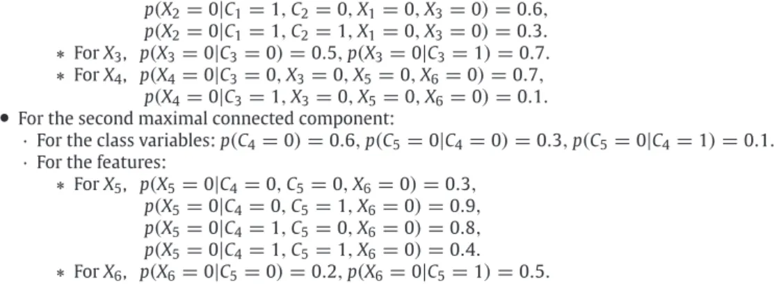
in (4) does not depend oni. Example 3(continued).Let xbe(
0,
0,
0,
0,
0,
0)
. Assume we have the following probabilistic information for theCB-decomposable MBC in Fig.5(a), where all variables (classes and features) are binary:
•
For the first maximal connected component:·
For the class variables:p(
C1=
0)
=
0.
3,
p(
C2=
0)
=
0.
6,
p(
C3=
0|
C2=
0)
=
0.
8,
p(
C3=
0|
C2=
1)
=
0.
4.
·
For the features:∗ ForX1, p
(
X1=
0|
C1=
0)
=
0.
2,
p(
X1=
0|
C1=
1)
=
0.
3∗ ForX2, p
(
X2=
0|
C1=
0,
C2=
0,
X1=
0,
X3=
0)
=
0.
2,
p
(
X2=
0|
C1=
1,
C2=
0,
X1=
0,
X3=
0)
=
0.
6,
p(
X2=
0|
C1=
1,
C2=
1,
X1=
0,
X3=
0)
=
0.
3.
∗ ForX3, p(
X3=
0|
C3=
0)
=
0.
5,
p(
X3=
0|
C3=
1)
=
0.
7.
∗ ForX4, p
(
X4=
0|
C3=
0,
X3=
0,
X5=
0,
X6=
0)
=
0.
7,
p
(
X4=
0|
C3=
1,
X3=
0,
X5=
0,
X6=
0)
=
0.
1.
•
For the second maximal connected component:·
For the class variables:p(
C4=
0)
=
0.
6,
p(
C5=
0|
C4=
0)
=
0.
3,
p(
C5=
0|
C4=
1)
=
0.
1.
·
For the features:∗ ForX5, p
(
X5=
0|
C4=
0,
C5=
0,
X6=
0)
=
0.
3,
p
(
X5=
0|
C4=
0,
C5=
1,
X6=
0)
=
0.
9,
p(
X5=
0|
C4=
1,
C5=
0,
X6=
0)
=
0.
8,
p(
X5=
0|
C4=
1,
C5=
1,
X6=
0)
=
0.
4.
∗ ForX6, p(
X6=
0|
C5=
0)
=
0.
2,
p(
X6=
0|
C5=
1)
=
0.
5.
Let
λ
be an additive CB-decomposable loss function given byλ(
c1, . . . ,
c5,
c1, . . . ,
c5)
=
λ
1(
c1,
c2,
c3,
c1,
c2,
c3)
+
λ
2(
c4,
c5,
c4,
c5),
where
λ
i(
c↓VCi,
c↓VCi)
=
dH(
c↓VCi,
c↓VCi)
, withi=
1,
2, anddHdenotes the Hamming distance, i.e. the number ofcoor-dinates wherec↓VCiandc↓VCiare different. Note that in our multi-dimensional classification problem,dHcounts the total
number of errors made by the classifier in the class variables. Thus,
λ
1isλ
1 (0,0,0) (0,0,1) (0,1,0) (0,1,1) (1,0,0) (1,0,1) (1,1,0) (1,1,1) (0,0,0) 0 1 1 2 1 2 2 3 (0,0,1) 1 0 2 1 3 1 3 2 (0,1,0) 1 2 0 1 2 3 1 2 (0,1,1) 2 1 1 0 3 2 2 1 (1,0,0) 1 3 2 3 0 1 1 2 (1,0,1) 2 1 3 2 1 0 2 1 (1,1,0) 2 3 1 2 1 2 0 1 (1,1,1) 3 2 2 1 2 1 1 0 andλ
2isλ
2 (0,0) (0,1) (1,0) (1,1) (0,0) 0 1 1 2 (0,1) 1 0 2 1 (1,0) 1 2 0 1 (1,1) 2 1 1 0 We have thatφ
x 1(
c1,
c2,
c3)
=
p(
c1)
p(
c2)
p(
c3|
c2)
·
p(
X1=
0|
c1)
p(
X2=
0|
c1,
c2,
X1=
0,
X3=
0)
p(
X3=
0|
c3)
·
p(
X4=
0|
c3,
X3=
0,
X5=
0,
X6=
0)
Table1lists the whole set of
φ
1xvalues on the left-hand side. The rest of the table develops the computations requiredforc∗↓VCias indicated in Corollary2. Therefore,c∗↓{C1,C2,C3}
=
(
1,
0,
0)
. Furthermore, we have thatφ
x2
(
c4,
c5)
=
p(
c4)
p(
c5|
c4)
p(
X5=
0|
c4,
c5,
X6=
0)
p(
X6=
0|
c5),
where the associated results are shown in Table2. Therefore,c∗↓{C4,C5}
=
(
0,
1)
.component. (c1,c2,c3) φ1x(c1,c2,c3) (c1,c2,c3) c1,c2,c3λ1φ1x (0, 0, 0) 0.0020160 (0, 0, 0) 0.0363048 (0, 0, 1) 0.0001008 (0, 0, 1) 0.0831432 (0, 1, 0) 0.0016800 (0, 1, 0) 0.0538776 (0, 1, 1) 0.0005040 (0, 1, 1) 0.0795480 (1, 0, 0) 0.0211680 (1, 0, 0) 0.0275016 (1, 0, 1) 0.0010584 (1, 0, 1) 0.0394632 (1, 1, 0) 0.0035280 (1, 1, 0) 0.0313656 (1, 1, 1) 0.0010584 (1, 1, 1) 0.0570360 Table 2
Computing the minimum expected loss in the second max-imal connected component.
(c4,c5) φx2(c4,c5) (c4,c5) c4,c5λ2φ x 2 (0, 0) 0.0108 (0, 0) 0.3394 (0, 1) 0.1890 (0, 1) 0.0956 (1, 0) 0.0064 (1, 0) 0.4608 (1, 1) 0.0720 (1, 1) 0.2170
Corollary 3. Under the same assumptions as in Theorem5with r
=
d maximal connected components, thenmin c∈IR
(
c|
x)
=
d i=1 min ci ciλ
i(
ci,
ci)
·
φ
ix(
ci)
j=i cjφ
x j(
cj),
whereφ
x i(
ci)
=
p(
ci)
X∈Ch(Ci) p(
x|
ci,
paVX(
x)).
Proof. The proof is straightforward from Theorem5. Under this decomposability, class variables are not longer conditioned
to other class variables.
Note that the simplest CB-decomposability applies in this case. 5. Performance evaluation metrics for multi-dimensional classifiers
We propose the following performance measures that extend metrics existing in the single-class domain. Cases i
∈
{
1, . . . ,
N}
are assumed to belong to the test data set.(1) Mean accuracy over thedclass variables:
Accd
=
1 d d j=1 Accj=
1 d d j=1 1 N N i=1δ(
cij,
cij),
(6)where
δ(
cij,
cij)
=
1 ifcij=
cij, and 0 otherwise. Note thatcij denotes theCjclass value outputted by the model forcaseiandcijis its true value.
A similar concept may be extended to CB-decomposable MBCs by means of the mean accuracy over thermaximal
connected components: Accr
=
1 r r j=1 1 N N i=1δ(
c↓i VCj,
c↓iVCj).
(2) Global accuracy over thed-dimensional class variable:
Acc
=
1 N N i=1δ(
ci,
ci)
(7)where
δ(
ci,
ci)
=
1 ifci=
ci, and 0 otherwise. Therefore, we call for an equality in all the components of the vector of predicted classes and the vector of real classes.It holds thatAcc
≤
Accr≤
Accd. This is obvious since it is less demanding to count errors in a component-wisefashion than as a vector of components that, as a whole, has to correctly predict all its coordinates. If all the class variables are binary, then we also have:
(3) MacroF1:
MacroF1
=
2Pred×
RecdPred
+
Recd,
(8)
where mean precision and mean recall over thedclass variables are defined, respectively, as
Pred
=
1 d d j=1 Prej,
Recd=
1 d d j=1 Recj.
Prejand Recjare the precision and recall, respectively, obtained from the single-class confusion matrix ofCj, i.e.
Prej
=
TPjTPj+FPj
,
Recj=
TP jTPj+FNj, whereTPj
,
FNj,TNj,
FPjare the counts for true positives, false negatives, true negativesand false positives, respectively.
(4) MicroF1: MicroF1
=
2Pre g×
Recg Preg+
Recg,
(9) where Preg=
d j=1TPj d j=1(
TPj+
FPj)
,
Recg=
d j=1TPj d j=1(
TPj+
FNj)
,
which could be seen as global precision and global recall. 6. Learning MBCs from dataIn this section we introduce algorithms to learn MBCs from data. LetDbe a database ofNobservations containing a
value assignment for each variableX1
, . . . ,
Xm,
C1, . . . ,
Cd, i.e.D= {
(
x(1),
c(1)), . . . , (
x(N),
c(N))
}
. The learning problemis to find an MBC that best fits the available data. We will use a score + search approach [10] to find the MBC structure.
MBC parameters can be estimated as in standard Bayesian networks. Thescoremeasuring the goodness of an MBC givenD
can be independent of or dependent on the classifier performance measure (a filter score or a wrapper score respectively)
[21,35]. Although any kind of strategy could be employed tosearchthe MBC space, the algorithms proposed below follow
a greedy search for computational reasons. The algorithms will, however, be flexible due to the possibility of incorporating filter, wrapper or hybrid approaches and because, as opposed to other proposals found in the literature, any kind of structure is allowed for the class and feature subgraphs.
6.1.pure filteralgorithm
Given a fixed ordering of all the variablesO
=
(
OC,
OX)
=
(
Cπ(1), . . . ,
Cπ(d),
Xπ(1), . . . ,
Xπ(m))
, whereπ
andπ
arepermutations over the variables inVCandVX, respectively, this algorithm first learns the class subgraph,GC, with a filter
score that takes into account orderingOC and then learns the feature subgraph,GX, usingOX in the same way, once the
bridge subgraph,GCX, is fixed.
The learning problem can be solved as two separate problems: (1) the search for the best structure ofGC, taking into
account only theDC
= {
c(1), . . . ,
c(N)}
values, which is solved once; and (2) the search for the best structure ofGX,constrained by fixed parents inVCgiven in a candidate bridge subgraphGCX, which is then updated via a best-first search in
GCX. By choosing a decomposable score, both searches, inGXandGCX, may reduce their computational burden considerably
since only local computations are carried out.
Considering the MBC structure, the global scores
(D
|
G)to be maximized, is the sum of the scores over the class variables,Fig. 6. Pseudocode of the pure filter algorithm.
Fig. 7. Pseudocode of the pure wrapper algorithm.
The algorithm is in Fig.6.
Note that the MBC structure and the ancestral fixed orderO
=
(
OC,
OX)
allow us to use data from the class variables,to search for the best class subgraph,GC∗, independently of the other variables (step 1). On the other hand, we organize
the search of the rest of the graph by first fixing a bridge subgraph (steps 2 and 5) and then searching for the best feature subgraph conditioned to the class parents given in the bridge subgraph (step 4). An example would be to apply a K2 algorithm
over the features usingOXbut with the bridge subgraph imposing some class variables as parents. Then, we move to a new
bridge subgraph which is equal to the previous one except for one added arc (step 3). This greedy strategy is handy from a computational point of view, since if we use a decomposable score, the new and old scores only differ by the term involving
the new arc. That is, when arc
(
Cl,
Xj)
∈
ACX is added to the bridge subgraphGCX(i)to have a candidate bridge subgraphGCX(i+1), then the difference required in step 5,sGCX(i+1)
(D
|
GX(i+1)
)
−
sGCX(i)
(D
|
GX(i)
)
, consists of the score only evaluatingXjand its new parents.
Note that the greedy strategy is forward, starting from the empty graph (step 2). Each time a better structure (bridge + features) is found (a better score), we update the current structure with this new one –a best-first strategy– and start the forward scheme from here. The process stops when any addition to the current bridge subgraph fails to provide a feature subgraph that improves the score.
6.2.pure wrapperalgorithm
This algorithm greedily searches for one arc, to be added or removed, in any position but respecting the MBC structure,
such that the global accuracyAcc, as defined in Section 5, is improved. Any general DAG structure is allowed for the class
and feature subgraphs. The algorithm stops if no arcs can be added or deleted to the current structure to improve the global accuracy.
The algorithm is in Fig.7.
This algorithm is controlled by theAccmeasure. Any other performance measure defined in Section 5 could be used.
However, computingAccinvolves the computation of the MPE for the class variables given the features, and this has the
advantage of being alleviated if there are CB-decomposable MBCs (Theorem3), which is likely to be the case as the algorithm
progresses, specially in the early stages. Also, gray codes will reduce the computations (Theorems4and2).
Special case of an additive CB-decomposable loss function.Let
λ(
c,
c)
be an additive CB-decomposable loss functionapplied with the following modifications. The global accuracyAcccounts the number of correctly classified cases based on the real and predicted class vectors. However, since the loss function is no any longer 0-1, the predicted class vector for each
xis obtained by minimizing its expected lossR
(
c|
x)
. Whenλ
is additive CB-decomposable, Theorems4and5and Corollary2provide computational savings via gray codes and MBC decomposability, which would be beneficial in step 2 of the algorithm.
Moreover, when trying to move to a new structure at step 2, if
λ
is additive CB-decomposable, the added/deleted arc shouldguarantee that a CB-decomposable MBC withrmaximal connected components according to
λ
is yielded. This means thatthe class subgraph is constrained by only allowing arcs among class variables of the same groupVCi
,
i=
1, . . . ,
rdefinedby
λ
. It also means that the non-shared children property for thercomponents should hold. Note that our forward strategystarting from the empty structure will produce structures withh
>
rmaximal connected components in the early iterations.These structures will be valid as long as they do not contradict the groups of class variables given by
λ
.6.3.hybridalgorithm
This algorithm is equal to thepure filteralgorithm but the decision on the candidate structures at step 5 is made based
on the global accuracyAcc(or any other performance measure), rather than on a general scores.
6.4. Cardinality of MBC structure space
The above learning algorithms move within the MBC structure space. Thus, knowledge of the cardinality of this space can help us to infer the complexity of the learning problem. We will point out two cases. The first one is the general MBC,
whereas the second one places two constraints on the MBC bridge subgraph sometimes found in the literature [70,15].
Theorem 6. The number of all possible MBC structures with d class variables and m feature variables, MBC
(
d,
m)
, is MBC(
d,
m)
=
S(
d)
·
2dm·
S(
m),
where S
(
n)
=
ni=1(
−
1)
i+1ni2i(n−i)S(
n−
i)
is Robinson’s formula [50] that counts the number of possible DAG structures of n nodes, which is initialized as S(
0)
=
S(
1)
=
1.Proof. S
(
d)
andS(
m)
count the possible DAG structures for the class subgraph and feature subgraph, respectively. 2dmisthe number of possible bridge subgraphs.
We now consider MBCs satisfying the following conditions on their bridge subgraph: (a) for eachXi
∈
VX, there is aCj
∈
VCwith(
Cj,
Xi)
∈
ACX and (b) for eachCj∈
VC, there is anXi∈
VX with(
Cj,
Xi)
∈
ACX. These conditions were usedin van der Gaag and de Waal [70] and in de Waal and van der Gaag [15] for learningtree–treeandpolytree–polytree
MBCs, respectively. The number of possible bridge subgraphs is given by the following theorem.
Theorem 7. The number of all possible bridge subgraphs, BRS
(
d,
m)
, m≥
d, for MBCs satisfying the two previous conditions (a) and (b) is given by the recursive formulaBRS
(
d,
m)
=
2dm−
m−1 k=0 dm k−
dm k=m x≤d,y≤m k≤xy≤dm−d d x m y BRS(
x,
y,
k),
where BRS
(
x,
y,
k)
denotes the number of bridge subgraphs with k arcs in an MBC with x class variables and y feature variables which is initialized as BRS(
1,
1,
1)
=
BRS(
1,
2,
2)
=
BRS(
2,
1,
2)
=
1.Proof. It holds that
BRS
(
d,
m)
=
dm k=max{d,m}=m BRS(
d,
m,
k)
=
dm k=m ⎡ ⎢ ⎢ ⎢ ⎣ dm k−
x≤d,y≤m k≤xy≤dm−d d x m y BRS(
x,
y,
k)
⎤ ⎥ ⎥ ⎥ ⎦=
2dm−
m−1 k=0 dm k−
dm k=m x≤d,y≤m k≤xy≤dm−d d x m y BRS(
x,
y,
k)
k
=
max{
d,
m} =
marcs. In the second equality,BRS(
d,
m,
k)
is computed by subtracting the bridge subgraphs not satisfyingthe two required conditions from the number of possible bridge subgraphs withkarcs, which isdmk. These “invalid” bridge
subgraphs include arcs fromxclass variables toyfeature variables, such thatx
≤
d,
y≤
mandk≤
xy≤
dm−
d.xymustbe at leastkto havekarcs in the bridge subgraph. Also,xymust be lower thandm
−
d+
1, which is the maximum numberof arcs for a valid bridge subgraph. Finally, the third equality is straightforward from the expansion of
(
1+
1)
dm.Theorem 8. The number of all possible MBC structures with d class variables and m feature variables, m
≥
d, satisfying conditions (a) and (b), MBCab(
d,
m)
isMBCab
(
d,
m)
=
S(
d)
·
BRS(
d,
m)
·
S(
m).
Proof. The proof is straightforward from Theorems6and7.
Corollary 4. The number of all possible MBC structures with d class variables and m feature variables satisfies O
(
MBC(
d,
m))
=
O(
MBCab(
d,
m))
=
2dm(
max{
d,
m}
)
2O(max{d,m}).
Proof. The complexity of Robinson’s formula [50] was shown to be super exponential, i.e.O
(
S(
n))
=
n2O(n). Also,O(
BRS(
d,
m))
=
2dm. Therefore,O
(
MBC(
d,
m))
=
O(
MBCab(
d,
m))
=
d2O(d)·
2dm·
m2O(m)≤
(
max{
d,
m}
)
2·2O(max{d,m})·
2dm=
2dm(
max{
d,
m}
)
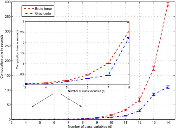
2O(max{d,m})7. Experimental results on MPE
An upper bound for the number of factors saved when computing the posterior probabilities of the MPE with gray codes
was given in Section3. This obviously has an effect on the required time. Here we compare the efficiency of the gray codes
against a brute force approach as exact algorithms for MPE computation.
The experiment consists of randomly generating 12 different MBCs with a number of binary class variables ranging from
d
=
3 tod=
14 and withm=
10 binary feature variables. First, a DAG generator produces a general class subgraphand a general feature subgraph. Second, the bridge subgraph is randomly generated. A data set with 10,000 cases is finally
simulated from the resulting MBC via probabilistic logic sampling [29]. We then compute ten MPE problems as in Eq. (2),
given ten random evidencesx(1)
, . . . ,
x(10). For the gray codes, computations are based on Corollary1.Fig.8shows error bars for computation times when using both exact approaches. They are obtained from the average
times over the ten MPE problems and the 12 different MBCs minus/plus the standard deviation.
Note that the gray code approach is faster than brute force, and this effect is more significant as the number of class
variables,d, increases. This is consistent with the bounds computed in Section3, sinceIanddappear in the denominator
of Theorem2.
8. Experimental results on learning MBCs
8.1. Data sets
For the purpose of our study, we use three benchmark data sets.2 Emotionsdata set [62] includes 593 sound clips
from a 30-seconds sequence after the initial 30 seconds of a song. The 72 features extracted fall into two categories: 8 rhythmic features and 64 timbre features. Songs are categorized by six class variables: amazed-surprised, happy-pleased, relaxing-calm, quiet-still, sad-lonely, and angry-aggressive.
TheScenedata set [4] has 2407 pictures, and their semantic scenes have to be classified into six class binary variables: beach, sunset, foliage, field, mountain, and urban. The 294 features correspond to spatial color moments in the LUV space.
TheYeastdata set [23] is about predicting the 14 functional classes of 2417 genes in the Saccharomyces Cerevisae Yeast. Each gene is described by the concatenation of microarray expression data and a phylogenetic profile given by 103 features.
All class variables are binary. The details of the three data sets are summarized in Table3.
However, feature variables are numeric. Since MBCs are defined for discrete variables, it is necessary to discretize all the continuous features. We use a static, global, supervised and top-down discretization algorithm called class-attribute
contingency coefficient [7]. TheEmotionsandScenedata sets contain some missing records. Missing records in the class
2
3 4 5 6 7 8 9 10 11 12 13 14 0 50 100 150 200 250 300 350 400
Number of class variables (d)
Computation time in seconds
Brute force Gray code 3 4 5 6 7 8 0 0.5 1 1.5 2 2.5 3
Number of class variables (d)
Computation time in seconds
Fig. 8. Error bars for running times when MPE is computed with gray code (blue) and brute force (red) approaches.
Table 3
Basic information of the three data sets.
Data set Domain Size m d
Emotions Music 593 72 6
Scene Vision 2407 294 6
Yeast Biology 2417 103 14
variables (only 0
.
16% forSceneand none forEmotions) were removed for MPE computations. When there are missingvalues in the feature variables (0
.
15% forSceneand 0.
11% forEmotions), MPE computations are carried out after theirimputation. In the estimation of (conditional) probabilities, we only consider the cases with no missing values for the variables involved.
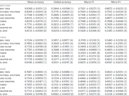
8.2. Experimental setup
We use eight different algorithms to learn MBCs. First, we apply five algorithms explicitly designed for MBCs:tree–tree
[70],polytree–polytree[15] andpure filter, pure wrapperandhybriddescribed in Section6.pure filterandhybridare implemented using the K2 algorithm. Second, we use two greedy search algorithms that learn a general Bayesian network,
one guided by the K2 metric [10] (filter approach), and the other guided by a performance evaluation metric, as defined in
Section5(wrapper approach). The first one will be denotedk2 bn, while the second one will bewrapper bn. Algorithmspure
filter, hybridandk2 bnrequire an ancestral ordering over the variables. We choose the best one after trying 1000 random
orderings forEmotionsandSceneand 100 random orderings forYeast, which has more class variables. Third, we consider
a multi-label lazy learning approach namedml-knn[72], see Section9.1, derived from the traditional K-nearest neighbor
algorithm. In this case, we set K to 3 in theEmotionsandScenedata sets, and 5 in theYeastdata set. As explained in
Section9.4, since it is unfeasible to compute the mutual information of two features givenallthe class variables, as required
in [15], we decided to implement thepolytree–polytreelearning algorithm using the (marginal) mutual information of
pairs of features. The heuristic searches always terminate after 200 unsuccessful trials looking for better structures, for
EmotionsandScene, and just 20 trials forYeast.
The probabilities attached to each node in the learnt network are calculated by maximum likeliho