Technische Universität Ilmenau
Institut für Mathematik
Preprint No. M 19/06
Solving multiobjective mixed integer
convex optimization problems
Marianna de Santis, Gabriele Eichfelder, Julia Niebling, Stefan Rocktäschel
Mai 2019
Impressum:
Hrsg.: Leiter des Instituts für Mathematik Weimarer Straße 25 98693 Ilmenau Tel.: +49 3677 69-3621 Fax: +49 3677 69-3270 http://www.tu-ilmenau.de/math/ URN: urn:nbn:de:gbv:ilm1-2019200296
Solving Multiobjective Mixed Integer
Convex Optimization Problems
Marianna de Santis
∗, Gabriele Eichfelder
∗∗, Julia Niebling
∗∗, Stefan Rockt¨
aschel
∗∗May 28, 2019
Abstract
Multiobjective mixed integer convex optimization refers to mathematical pro-gramming problems where more than one convex objective function needs to be optimized simultaneously and some of the variables are constrained to take integer values. We present a branch-and-bound method based on the use of properly de-fined lower bounds. We do not simply rely on convex relaxations, but we built linear outer approximations of the image set in an adaptive way. We are able to guaran-tee correctness in terms of detecting both the efficient and the nondominated set of multiobjective mixed integer convex problems according to a prescribed precision. As far as we know, the procedure we present is the first deterministic algorithm devised to handle this class of problems. Our numerical experiments show results on biobjective and triobjective mixed integer convex instances.
Key Words: Multiobjective Optimization, Mixed Integer Convex Programming
Mathematics subject classifications (MSC 2010): 90C11, 90C26, 90C29
1
Introduction
Multiobjective programming is concerned with mathematical problems where more than one objective function needs to be optimized simultaneously. When the problem considered involves both continuous and integer variables we are in the context of multiobjective mixed integer programming. In this paper, we focus on multiobjective mixed integer convex programming problems, namely problems of the following form:
min (f1(x), . . . , fm(x))T
s.t. gk(x)≤0 k = 1, . . . , p
x∈B := [l, u]
xi ∈Z ∀i∈I,
(MOMIC)
∗Department of Computer, Control and Management Engineering, Sapienza Universit`a di Roma, Via
Ariosto 25 00185 Roma, Italy,[email protected]
∗∗Institute for Mathematics, Technische Universit¨at Ilmenau, Po 10 05 65, D-98684 Ilmenau, Germany,
where fj, gk : B → R; j = 1, . . . , m; k = 1, . . . , p are convex and continuously
differ-entiable functions. The vectors l, u ∈ Rn are lower and upper bounds on the decision
variables x ∈ Rn and define the box B. The index set I ⊆ {1, . . . , n} specifies which
variables have to take integer values. We assume w.l.o.g. li, ui ∈ Z for all i ∈ I. The
image of the feasible set of the problem under the vector-valued function f : Rn → Rm
represents the feasible set in the criterion space, or the image set.
Multiobjective mixed integer optimization problems arise in many application fields such as location or production planning, finance, manufacturing, and emergency manage-ment (see e.g. [14, 28, 30]). As an example we can think of the uncapacitated facility location problem, studied in the single-objective case in [18]. The first objective hereby is to decide which facilities to build in order to minimize costs. As a second objective func-tion one could consider the total negative impact on the environment with the building plan for the facilities, e.g. the carbon emissions.
Solving a multiobjective optimization problem aims at detecting the efficient set, namely the set of points in the decision space that leads to nondominated points in the criterion space. A point of the image set is nondominated if none of its components can be decreased without increasing any other component. A formal definition will be given in Section 2.
It is well known that mixed integer nonlinear optimization is NP-hard and its solution typically requires dealing with enormous search trees [1]. Handling more than one objective function adds an additional difficulty: assume there is only one binary variable, I = 1 with x1 ∈ {0,1}, and we have just one objective function, i. e., m = 1. Then for solving
(MOMIC) only two convex optimization problems have to be addressed, one withx1 fixed
to 0 and one withx1 fixed to 1. Clearly, the smallest minimal value is the optimal value of
the original problem. In case of two or more objective functions already this simple setting is much more challenging. Solving the problems with fixed values for x1 would mean to
determine the whole efficient set of a multiobjective convex optimization problem, which is in general infinite. Then, after computing two sets of nondominated points one has to compare them and to determine the “smallest” values, see Figure 1 on page 5 for an illustration of this observation for four choices of the integer variables.
So far, there exist mostly algorithms for solving multiobjective mixed integer linear
programming problems only. Those can be divided into two main classes: decision space search algorithms, i.e., approaches that work in the space of feasible points, and criterion space search algorithms, i.e., methods that work in the space of objective function values. Among the decision space search algorithms, the method proposed by Mavrotas and Diakoulaki, [24], is the first branch-and-bound algorithm for solving multiobjective mixed binary programs. The authors improved and extended their work in [23, 25]. Other works defining branch-and-bound algorithms for multiobjective integer linear program-ming problems are [12, 29]. There, in the bounding procedure the aim is to define proper hypersurfaces in the objective space in order to separate the upper and lower bound sets. Criterion space search algorithms find nondominated points by addressing a sequence of single-objective optimization problems. Once a nondominated point is computed, dom-inated parts of the criterion space are removed and the algorithms go on looking for new nondominated points. Several contributions in the context of criterion space search algo-rithms for biobjective and triobjective mixed integer linear programming have been given
by Boland and co-authors [2, 3,4, 5].
As far as we know, the first general purpose method to tackle multiobjective mixed integerconvex programs is the heuristic based on a branch-and-bound algorithm proposed by Cacchiani and D’Ambrosio in [10].
A classical technique to solve a multiobjective optimization problem is to convert the problem into a parameter-dependent single-objective one, known as scalarization. This approach was recently followed by Burachik et al. [8] (see also the comment in the con-clusions of [9]). The scalarized problems are then parameter-dependent single-objective mixed integer convex optimization problems. By following this approach, many of these single-objective problems have to be solved, one for each choice of the parameter’s value. No gained information of pre-solved problems are typically used thereby. Furthermore, it is not clear how to choose the parameter’s values in a smart way and this is an open challenge: as the set of nondominated points is in general disconnected and can have huge gaps, many subproblems defined according to different parameter’s values might lead to the same nondominated point and thus solving such subproblems is a wasted effort.
We propose in this paper for the first time a deterministic algorithm for multiobjective mixed integer convex problems which is not using a scalarization of the original problem. We directly develop a branch-and-bound algorithm based on a partitioning of the feasible region, i.e., a decision space algorithm. We present two versions of the algorithm. In one version we do not have to solve any single-objective mixed integer subproblem but only single-objective convex subproblems. In the second version we need to address also single-objective mixed integer convex optimization problems. No parameter needs to be chosen to define the subproblems we consider.
To compute lower bounds in our branch-and-bound approach we rely on linear outer approximations of the image set. We use outer approximation techniques from convex multiobjective optimization for finding lower bounds of the continuous relaxation of the problem (i. e., the problem obtained by ignoring the integrality constraints), as well as for constructing outer approximations of the convex hull of the true image set over subboxes. We keep track of upper bounds in the image space and derive by that a discarding test for the branch-and-bound procedure. This results in a deterministic solver for which we can give theoretical guarantees to find approximations of the set of efficient and of the set of nondominated points.
The paper is organized as follows. In Section 2 we report notations and definitions that will be used throughout the paper. In Section 3 we present our branch-and-bound algorithmMOMIX. Details on how to define a “light” version of the algorithm that does not need to address any single-objective mixed integer convex programming problem are given as well. Theoretical insights of MOMIX and MOMIXlight are also given in Section 3. Some
numerical results are reported in Section 4. Section 5concludes.
2
Definitions and Notations
Throughout the paper, we indicate with k · k the Euclidean norm. Given a boxB = [l, u], we denote by ω(B) its width obtained as the Euclidean distance between l and u, namely
ω(B) =ku−lk. Given two vectors x, y ∈ Rn, we write x ≤ y and x < y if x
xi < yi for all i ∈ {1, . . . , n}, respectively. We write x y when an index i ∈ {1, . . . , n}
exists such thatxi > yi. Given a vectorx∈Rnand an index setI ⊆ {1, . . . , n}, we denote
with xI the subvector with componentsxi, i∈I.
Let x∈R, we define
bxc:= max{c∈Z|c≤x},dxe:= min{c∈Z|x≤c} and [x] :=
(
dxe if x+ 0.5≥ dxe bxc otherwise.
Forx∈Rn, we define bxc, dxeand [x] componentwise.
For a nonempty set A ⊂Rm, we denote by conv(A) the convex hull of A, namely the
smallest convex set that contains A. By Bg, BZ and Bg,Z we denote the following sets
related to the constraints in (MOMIC):
Bg :={x∈B |g(x)≤0},
BZ :={x∈B |x
i ∈Z for all i∈I},
Bg,Z :=Bg∩BZ.
(1)
Using these sets, we can write (MOMIC) in compact form as min f(x)
s.t. x∈Bg,Z.
As mentioned, we are going to define a branch-and-bound method based on partitioning the feasible set of (MOMIC). Our branching rule is based on bisections of the box B. Let
˜
B be a subbox of B. By ˜Bg, ˜BZ and ˜Bg,Z we denote the sets defined according to (1),
where the set B is replaced by ˜B (i.e., x∈B˜ in all the set definitions).
We recall here the basic concepts of efficient and nondominated points (see [20] for further details).
Definition 2.1 (a) A feasible pointx∗ ∈Bg,Zis efficient for (MOMIC)if there is nox∈
Bg,Z with f(x) ≤f(x∗) andf(x)6=f(x∗). The set of efficient points for (MOMIC)
is the efficient set of (MOMIC).
(b) A point z∗ =f(x∗) is nondominated for (MOMIC) ifx∗ ∈Bg,Z is an efficient point
for (MOMIC). The set of all nondominated points of (MOMIC)is the nondominated set of (MOMIC).
(c) Letx, x∗ ∈Bg,Z with f(x)≤f(x∗) andf(x)6=f(x∗). Then we say thatx dominates
x∗ and also that f(x) dominates f(x∗).
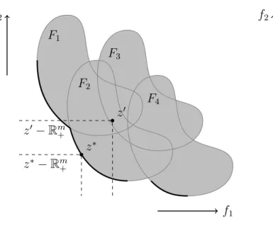
In Figure 1, we plot the image set of a biobjective mixed integer convex optimization problem. Here, we assume that {xI | x ∈ Bg,Z} =: {y1, y2, y3, y4} and we show the sets
Fj := {f(x) | x ∈ Bg,Z, xI = yj}, j = 1, . . . ,4. Then, S
j=1,...,4Fj = {f(x) | x ∈ Bg,Z}.
The point z∗ ∈ f(Bg,Z) is nondominated and the preimage of z∗ is an efficient point.
On the other hand, z0 ∈ f(Bg,Z) is dominated because z∗ ≤ z0 and z∗ 6= z0. In fact,
all the points z ∈ F3 are dominated, as points w ∈ f(Bg,Z) exist such that w < z. The
z∗−Rm + z∗ F1 F2 F3 F4 z0−Rm + z0 f1 f2
Figure 1: Image set of a biobjective in-stance of (MOMIC). z−Rm + z f( ˜Bg,Z) LB˜ f1 f2
Figure 2: Image set of a biobjective purely integer instance of (MOMIC).
efficient set is made of all preimages of the nondominated set. Figure 1 shows that the nondominated set of a multiobjective mixed integer nonlinear programming problem is in general a disconnected set. From an algorithmic point of view, this makes the detection of the efficient set of (MOMIC) an extremely challenging problem. Furthermore, there is the necessity of comparing sets of points: this is a crucial difference with respect to single-objective mixed integer nonlinear optimization.
3
MOMIX
: An Outer Approximation based
Branch-and-Bound Algorithm for (MOMIC)
The algorithm we propose is a branch-and-bound method that looks for the efficient set of (MOMIC) by partitioning the box B. At every node of the branch-and-bound tree, a subbox ˜B ⊆ B is selected and lower and upper bounds on the nondominated set of (MOMIC) are derived. When considering the subbox ˜B, a lower bound is any set
LB˜ ⊆Rm such thatLB˜+Rm+ contains the image of integer feasible points ˜Bg,Z through f,
namely f( ˜Bg,Z)⊆L˜
B+Rm+. In Figure 2, we illustrate the set f( ˜Bg,Z) and a lower bound
LB˜ for a biobjective purely integer programming problem: note that the image of feasible
points in ˜B through f is a set of isolated points in Rm.
In our algorithm we derive lower bounds by building linear outer approximations of conv(f( ˜Bg,Z)). As f( ˜Bg,Z)⊆ conv(f( ˜Bg,Z)), we have that linear outer approximations of
hyperplanes to outer approximate conv(f( ˜Bg,Z)) will be given in Section 3.2.
Upper bounds are computed just by evaluating the objective functions at feasible points. As soon as an upper bound z exists such that LB˜ +R+m ⊆ {z}+Rm+ \{0} we can
discard the subbox ˜B. Or, in other words, we can avoid to go on partitioning ˜B, as we have an evidence that it cannot contain any efficient point for (MOMIC). Our discarding procedure is in fact using a list of upper bounds and it will be detailed in Section3.1 and Section3.2.
In Figure 2, the point z ∈ f( ˜Bg,Z) is an upper bound for the nondominated set of
the problem, as it is the image of an integer feasible point. All the points that belong to
Rm\({z}+Rm+ \ {0}) are candidates to belong to the nondominated set (note that it is
not enough to consider{z} −Rm
+).
Let δ >0 be a positive scalar, which is the input parameter of our branch-and-bound method. As the output of our algorithm, we will have a list of subboxes ˜B with ω( ˜B)< δ, containing the set of efficient points, and a list of upper bounds approximating the nondominated set.
Algorithm 1 is a basic scheme of our branch-and-bound procedure: LW denotes the
working list and contains boxes that still have to be examined. The list LS denotes the
list of boxes that fulfill the termination criteria, i.e., those subboxes ˜B that were not discarded and satisfyω( ˜B)< δ. In Section 3.3 we will prove thatLS represents a cover of
the efficient set E, namely E ⊆ S
˜
B∈LS
˜
B. The list LP N S denotes a set of upper bounds
and it will be defined in Section3.1. Note that the flagDis used in order to decide if a box should be discarded, and it is an output of Algorithm2. As a final step in Algorithm1we filter the listLS by a postprocessing phase. Further details will be given in Section 3.2.
3.1
Computation of upper bounds and local upper bounds
In order to compute upper bounds of the nondominated set of (MOMIC), we evaluate the objective functions at integer feasible points x∈ Bg,Z. It is well known that determining
feasible points of a mixed integer set is an NP-hard problem. In the literature, several heuristic methods have been proposed and we cite the Feasibility Pump [15] and some of its enhancements, among them [6, 7, 11, 16]. Within our algorithm, we either detect feasible points by addressing specific single-objective mixed integer convex programming problems (see Section3.2) or we try to build feasible points simply by rounding the integer components of points x∈B˜, which are generated in our discarding test. Let round(x) be the point defined as
round(x) =
[xi] i∈I
xi otherwise.
If round(x)∈Bg,Z holds, f(round(x)) is a valid upper bound.
Upper bounds are needed in order to discard boxes or, in other words, to prune nodes in the branch-and-bound tree. In order to do that we need to introduce two finite sets of points, namely the list of potentially nondominated solutions LP N S ⊆f(Bg,Z) and the list
of local upper bounds LLU B ⊆Rm.
In our algorithm the list of potentially nondominated solutions LP N S is initialized as
Algorithm 1 MOMIX: a (MOMIC) Solver
INPUT: (MOMIC),δ >0
OUTPUT:LS , LP N S
1: LS ← ∅ LW ← {B} LP N S ← ∅ 2: while LW 6=∅ do
3: Select a box ˜B of LW and update LW :=LW\B˜
4: Bisect ˜B into subboxes ˜B1 and ˜B2 5: for k = 1,2 do
6: Apply Algorithm 2 to ˜Bk and obtain D and an updated LP N S 7: if D=true then 8: Discard ˜Bk 9: else 10: if ω( ˜Bk)< δ then 11: Add ˜Bk to L S 12: else 13: Add ˜Bk to L W. 14: end if 15: end if 16: end for 17: end while 18: Postprocessing(LS,LP N S)
whether it is dominated by any point inLP N S. If this is the case, z is not added to LP N S.
Otherwise, we update the list by adding z to LP N S and by removing from LP N S all the
upper bounds dominated by z. By doing this, we ensure that LP N S is a stable set of
points: a set N ⊆Rm is said to be stable if there are nox, y ∈ N with x≤y and x6=y.
For the list of local upper bounds LLU B we need the following definition:
Definition 3.1 [21] Let N ⊆f(B) be a finite and stable set of points and Z ⊆ Rm be a
box such that f(B)⊆int(Z).
(a) The search region related to N and Z is defined as
S :={w∈int(Z)|z w for all z ∈ N }.
(b) The search zone for some p∈Rm related to Z is defined as
C(p) = {w∈int(Z)|w < p}.
(c) A list L ⊆ Z is called a local upper bound set with respect to N, if
(i) S =S
p∈LC(p)
Let Z ⊆ Rm be a box such that f(B) ⊆ int(Z). In our algorithm we initialize the
local upper bound set LLU B with the point p0 ∈ Rm defined as p0j := maxw∈Zwj. Then
we build and keep updatedLLU B with respect to the finite and stable set LP N S according
to the procedure proposed in [21]. For an illustration of the local upper bound set LLU B
with respect toLP N S, see Figure 3on page 9.
Remark 3.2 Along the iterations of our algorithm, letL0
P N S andLP N S be two consecutive
lists of potentially nondominated points, and let L0
LU B and LLU B be the related local upper
bound sets. Then, based on the update procedure mentioned above, we have that to any
z0 ∈ L0
P N S there exists z ∈ LP N S with either z0 = z or with z ≤ z0. Hence, the search
regions S0 and S related to L0
P N S and LP N S are such that S ⊆S0, i.e.,
S= [ p∈LLU B C(p) ⊆ [ p∈L0 LU B C(p) =S0.
Furthermore, for every p ∈ LLU B there exists a local upper bound p0 ∈ L0LU B such that
p≤p0. This can be seen by induction considering the updating procedure proposed in [21].
Note that p ∈ LLU B is not necessarily the image of a feasible point. Local upper
bounds are used in order to decide if a subbox ˜B ⊆B should be discarded as clarified by the following results.
Lemma 3.3 [26] Let LLU B be a local upper bound set with respect to the finite and stable
set LP N S ⊆f(Bg,Z). For every z∈ LP N S and for everyj ∈ {1, ..., m} there is a p∈ LLU B
with zj =pj and zr < pr for all r∈ {1, ..., m} \ {j}.
Based on this lemma we can prove our main result for the pruning of nodes:
Theorem 3.4 Consider a subbox B˜ ⊆B. Let LP N S ⊆f(Bg,Z) be a finite and stable set.
Let LLU B be the local upper bound set w.r.t. LP N S. If
p /∈f( ˜Bg,Z) +
Rm+ holds for all p∈ LLU B, (2)
˜
B does not contain any efficient point for (MOMIC).
Proof. Assume by contradiction that an efficient point x∗ ∈ B˜g,Z for (MOMIC) exists.
Therefore, from (2), we have
f(x∗)p for all p∈ LLU B. (3)
Since LLU B is a local upper bound set w.r.t. LP N S, it follows from (3) and Definition3.1
(b) and (c), thatf(x∗) does not belong to the search region S. Hence, there exists a point
z ∈ LP N S with z ≤ f(x∗). As z ∈ LP N S, a point x0 ∈ Bg,Z exists such that z = f(x0).
Since x∗ is efficient for (MOMIC), it follows z = f(x0) = f(x∗). Lemma 3.3 implies that there is a pointp0 ∈ LLU B withf(x∗)≤p0, which is a contradiction to (3) and the theorem
is proved.
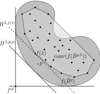
From Theorem 3.4, since ˜Bg,Z ⊆B˜g and f( ˜Bg,Z)⊆conv(f( ˜Bg,Z)) hold, we obtain the
Z f1 f2 LP N S LLU B f( ˜Bg)
Figure 3: Illustration of Corollary 3.5 for m = 2. In the picture we plot the local upper bound setLLU B with respect to the set of potentially nondominated solutionsLP N S. Note
that the box ˜B would be discarded, as the assumptions of Corollary 3.5 (a) are satisfied and ˜B cannot contain any efficient point for (MOMIC).
Corollary 3.5 Let B˜ be a subbox of B. Let LP N S ⊆f(Bg,Z) be a finite and stable set and
let LLU B be the local upper bound set w.r.t. LP N S.
(a) If
p /∈f( ˜Bg) +Rm+ holds for all p∈ LLU B,
˜
B does not contain any efficient point for (MOMIC). (b) If
p /∈conv(f( ˜Bg,Z)) +
Rm+ holds for all p∈ LLU B,
˜
B does not contain any efficient point for (MOMIC).
An illustration of Corollary 3.5 (a) can be found in Figure3.
The following remark clarifies how the assumptions of Corollary 3.5 are related. Fur-thermore, it gives the basis of the hierarchy of lower bounds in our bounding procedure.
Remark 3.6 Note that due to the convexity of the objective functions fj, j = 1, . . . , m
and of B˜g the following holds
conv(f( ˜Bg,Z)) +
Rm+ ⊆f( ˜B
g) +
Rm+.
3.2
Determining lower bounds and pruning nodes
The theoretical results introduced in the previous section, namely Corollary 3.5, give the basis of the discarding procedure in our branch-and-bound algorithm: For every subbox
˜
B we want to check whether p6∈LB˜ +R+m holds for all p∈ LLU B, being LB˜ a valid lower
bound for ˜Bg,Z.
As f( ˜Bg) is a valid lower bound, a straightforward way to verify if a box should be discarded would be to check whether a local upper bound p∈ LLU B belongs to this lower
bound given by the convex relaxation. This would mean to check whetherp∈f( ˜Bg)+
Rm+.
This can be done by addressing a simple single-objective continuous convex problem. From a computational point of view, this means that we would need to solve |LLU B|
single-objective continuous convex problems, at every node of the branching tree.
In our algorithm, in order to reduce this numerical effort, we check instead whether a local upper bound belongs to a linear outer approximation off( ˜Bg)+Rm+, i.e., we only need to check whether a local upper bound satisfies linear inequalities. Furthermore, our linear outer approximations are built in a smart way: the supporting hyperplanes computation is adaptively driven by some “meaningful” local upper bounds p∈ LLU B.
Additionally, in case we want to improve our lower bound, we compute further hy-perplanes to outer approximate conv(f( ˜Bg,Z)) +
Rm+. Again this computation is done in
an adaptive way, and the supporting hyperplanes computation is steered by some specific local upper bounds p∈ LLU B.
In the following, we give details on how the supporting hyperplanes are computed and how the discarding procedure works.
At an arbitrary node of our branching tree we select a subbox ˜B ⊆B. In order to com-pute valid lower bounds on ˜B we build linear outer approximations LB˜ of conv(f( ˜Bg,Z)),
so that f( ˜Bg,Z)⊆conv(f( ˜Bg,Z))⊆L ˜ B+R m +.
In order to discard the subbox ˜B and prune the current node we check whether
p6∈LB˜ +Rm holds for all p∈ LLU B.
Then, from Corollary 3.5B˜ does not contain any efficient point for (MOMIC) and the current node can be pruned. As we will deal with linear outer approximations of sets, we recall here the definition of supporting hyperplane of a set:
Definition 3.7 Let P ⊂Rm be a nonempty set, let λ ∈
Rm\ {0} and z ∈ ∂P, where ∂P
is the boundary of the set P. The hyperplane
Hλ,z :={y∈Rm |λTy=λTz}
is called supporting hyperplane (of P), if λTy≥λTz holds for all y∈P.
As mentioned in the introduction, we propose two versions of our branch-and-bound algorithm. The difference lies in the lower bounds computation. The first version of our algorithm, named MOMIXlight, computes valid lower bounds by addressing only
single-objective continuous convex optimization problems. The second version, named MOMIX, tries to define stronger lower bounds by dealing also with single-objective mixed integer convex programming problems. In our algorithm we use a flaglightto distinguish between the two versions of the method.
Both, MOMIXlight and MOMIX, start by computing linear outer approximations of the
convex setf( ˜Bg) +Rm+ by solving a family of single-objective continuous convex optimiza-tion problems. As conv(f( ˜Bg,Z)) +
Rm+ ⊆f( ˜Bg) +Rm+ holds by Remark 3.6, we have that
linear outer approximations of f( ˜Bg) +
Rm+ are valid lower bounds for conv(f( ˜Bg,Z)) as
not allow to discard the box ˜B, MOMIX tries to improve it by addressing properly defined single-objective mixed integer convex programming problems.
As a first step for the outer approximation, we compute the ideal point fid ∈
Rm of f( ˜Bg), namely the point whose j-th component is the minimum of f
j on ˜Bg:
fjid := min
x∈B˜g
fj(x) j = 1, . . . , m. (4)
We denote by xj,id ∈ B˜g a minimal solution in (4). Let ej be the j-th unit vector, then
Hej,fid is a supporting hyperplane off( ˜Bg). As a first linear outer approximation off( ˜Bg)
or, in other words, as a first lower bound for f( ˜Bg,Z) we consider
LB˜ :=∂ \ j∈{1,...,m} (Hej,fid +Rm+) ! ={fid}+∂(Rm+). (5)
Note that buildingLB˜ requires to solvemsingle-objective continuous convex optimization
problems for the computation of fid.
Once LB˜ is computed we enter in a loop. For every p ∈ LLU B we check whether
p ∈ LB˜ + Rm+ holds. If this is the case, we try to improve the current linear outer
approximation LB˜ by computing a further hyperplane, based on p ∈ LLU B. This is done
by addressing the following single-objective continuous convex programming problem (see also [13,22]) min t s.t. f(x)≤p+te x∈B˜g t∈R, (Pp( ˜Bg)) where e= (1, . . . ,1)T ∈ Rm.
Note that Problem (Pp( ˜Bg)) needs to be addressedonlyin case ofp∈LB˜+Rm+. In other
words, in our lower bound computation, we do not necessarily address Problem (Pp( ˜Bg))
for all p ∈ LLU B, as it would be the case if we would rely only on the convex relaxation
f( ˜Bg).
Under regularity assumptions, we have that any minimal solution (ˆx,ˆt) ∈ B˜g ×
R of
Problem (Pp( ˜Bg)) admits Lagrange multipliers. We refer to [13, 26] in case no Lagrange
multiplier exists. Let (ˆx,tˆ)∈ B˜g ×R be a minimal solution of (Pp( ˜Bg)) and let ˆλ ∈ Rm+
be a Lagrange multiplier for the constraint f(x) ≤ p+te. Then, the hyperplane Hλ,ˆyˆ(p)
with ˆy(p) :=p+ ˆte is a supporting hyperplane of f( ˜Bg), cf. [22, 27,26]. There exist two possibilities:
(i) If ˆt >0 holds, thenp /∈f( ˜Bg) +Rm+, we improve the outer approximation by Hˆλ,yˆ(p), and consider the next local upper bound;
(ii) if ˆt ≤0 holds, then p ∈f( ˜Bg) +
Rm+ and the assumption of Corollary 3.5 (a) is not
If case (ii) occurs, so far we cannot discard ˜B based on Corollary 3.5 (a) as it may contain efficient points for (MOMIC). Then, in case we apply MOMIX, i.e., light = 0, we try to apply Corollary3.5 (b) and thus we try to improve our linear outer approximation by addressing a single-objective mixed integer convex programming problem. Let ˆλ∈Rm
be a Lagrange multiplier for the constraintf(x)≤p+te for the solution of (Pp( ˜Bg)). We
define the following problem
min ˆλTf(x)
s.t. x∈B˜g,Z. (MICPp(ˆλ,
˜
B)) Let ˆx ∈ B˜g,Z be a minimal solution of (MICP
p(ˆλ,B˜)). Then the hyperplane H ˆ
λ,f(ˆx) is a
supporting hyperplane of conv(f( ˜Bg,Z)) and it holds conv(f( ˜Bg,Z)) +
Rm+ ⊆H ˆ
λ,f(ˆx)+
Rm+.
Furthermore, f(ˆx) is a valid upper bound for (MOMIC). Note that in case we are at a node where all integer variables are fixed we do not need to perform this step.
Again two situations occur:
(i) If ˆλTp <λˆTf(ˆx) holds, we improve the outer approximation by Hλ,fˆ (ˆx) and consider
the next local upper bound
(ii) If ˆλTp≥λˆTf(ˆx) holds, the local upper boundp lies above the hyperplane Hˆλ,f(ˆx). If we are in case (ii), we do not go on improving our linear outer approximation and we branch the current node by bisecting ˜B in a later iteration.
Algorithm 2is reporting our lower bound computation in details. As soon as feasible points of ˜Bg,Z are found, both L
P N S and LLU B are updated. This
is the reason why in Algorithm 2 we make use of the list L∗
LU B which does not change
along the discarding test: We need a fixed set of local upper bounds in order to ensure the termination of the loop starting in line10.
Note that in line 17we update the linear outer approximation even if the subbox ˜B is further kept either in the working list LW or in the solution list LS. This is done in order
to perform the postprocessing phase in Algorithm 1: Let ˜B ∈ LS and let H be the linear
outer approximation of f( ˜Bg,Z) built by Algorithm 2. This subbox ˜B is removed from L
S
if for all local upper bounds pbelonging to the final list LLU B we have that a hyperplane
Hλ,z0 ∈ H exists such that λTp≥λTz0 holds.
Example 3.8 In Figure 4 on page 14 we illustrate our lower bounding procedure on a biobjective purely integer convex programming instance. Note that in this case the image of integer feasible points is a set of isolated points in R2. The first outer approximation
considered is based on the ideal point fid. Then, considering the local upper bound p ∈
LLU B, the supporting hyperplane H
ˆ
λ,yˆ(p) for f( ˜Bg) is built by solving Problem (P
p( ˜Bg))
and added to the linear outer approximation. Finally, in case MOMIX (and not MOMIXlight)
is applied, the linear outer approximation is further refined by considering Hˆλ,f(ˆx), being
ˆ
x a solution of (MICPp(ˆλ,B˜)).
In the following lemma, we prove the exactness of our lower bounding procedure: we show that Algorithm 2 returns D = false in case ˜B contains an efficient point for (MOMIC). Thus it will be further partitioned.
Algorithm 2 Lower bounding procedure
INPUT: (MOMIC), a subbox ˜B ⊆B, LP N S,LLU B, light∈ {0,1} OUTPUT:LP N S, LLU B,D, whereD=true means “Discard ˜B”
1: Set D ←true
2: for j ∈ {1, . . . , m} do
3: Compute fjid and obtain xj,id ∈B˜g
4: if round(xj,id)∈Bg,Z then
5: Update LP N S by f(round(xj,id)) and update LLU B 6: end if 7: end for 8: Set L∗ LU B ← LLU B 9: Set H ← {Hej,fid |j ∈ {1, ..., m}} 10: for p∈ L∗LU B do
11: if λTp≥λTz0 for all Hλ,z0 ∈ H then
12: Solve (Pp( ˜Bg)) and get (x∗, t∗) ∈ B˜g ×R, ˆλ ∈ Rm Lagrange multiplier for
the constraint f(x)≤p+te
13: if round(x∗)∈Bg,Z then
14: UpdateLP N S byf(round(x∗)) and update LLU B 15: end if
16: if t∗ ≤0 and light= 1 then 17: Set H ← H ∪ {Hλ,pˆ +t∗e}
18: Set D ←false and break for-loop 19: else if t∗ ≤0 and light= 0 then
20: Solve Problem (MICPp(ˆλ,B˜)) 21: if (MICPp(ˆλ,B˜)) is infeasible then 22: Set D ← trueand break for-loop
23: else
24: Let ˆx∈B˜g,Z be a solution of Problem (MICP
p(ˆλ,B˜)) 25: Update LP N S byf(ˆx) and update LLU B
26: Set H ← H ∪ {Hˆλ,f(ˆx)} 27: end if
28: if λˆTp≥λˆTf(ˆx)then
29: Set D ← false and break for-loop 30: end if 31: else 32: Set H ← H ∪ {Hλ,pˆ +t∗e}. 33: end if 34: end if 35: end for
p fid f(ˆx) Hλ,ˆyˆ(p) Hλ,fˆ (ˆx) f( ˜Bg) conv(f( ˜Bg,Z))
Figure 4: Illustration of our lower bounding procedure on a biobjective purely integer convex programming instance.
Lemma 3.9 LetB˜be a subbox ofB that contains an efficient pointx∗ ∈B˜g,Zof (MOMIC).
Then Algorithm 2 returns D=false.
Proof. We distinguish two cases for which Algorithm2returnsD =true: eitherD =true
because (MICPp(ˆλ,B˜)) is infeasible for any p∈ L∗LU B or because lines 18 or29 are never
reached for anyp∈ L∗
LU B. The first case cannot occur asx∗ ∈B˜g,Z. The second case may
occur if for all p∈ L∗
LU B either the condition in line 11 or the condition in line 16 or the
condition in line 28 is not satisfied. In all three cases we get that p /∈ f( ˜Bg) +
Rm+ holds
for all p∈ L∗
LU B. Corollary 3.5 then implies that ˜B does not contain any efficient point
for (MOMIC).
3.3
Correctness of
MOMIX
We already mentioned that our algorithm stops as soon as the working list LW is empty
and we get a list of subboxes ˜B of width less than a prescribed valueδ >0, i.e., ω( ˜B)< δ. In this section we first prove the exacteness of Algorithm1, namely we prove that it returns the set LS which is a cover of the efficient set E of (MOMIC). In order to do that, we
need to make the following assumption related to the branching rule adopted.
Assumption 3.10 Let B˜ ⊆B. Let the branching rule in Algorithm 1be such that for the subboxes B˜1 and B˜2 derived from B˜ it holds
˜
Bg,Z⊆B˜1∪B˜2
and that the algorithm performs a finite number of branching steps before stopping.
Note that Assumption 3.10 implies that the set of efficient points for (MOMIC) be-longing to ˜B is a subset of ˜B1∪B˜2. In Section 4 we propose and compare two branching
rules which both satisfy Assumption 3.10.
Theorem 3.11 Let E be the efficient set of (MOMIC). Let LS be the output of
Algo-rithm 1. Then LS is a cover of E, namely E ⊆SB˜∈LSB˜.
We want to underline that when MOMIX (and not MOMIXlight) is applied, the list LS is
built in a way such that every subbox ˜B belonging toLS admits at least one feasible point,
i.e., ˜Bg,Z 6=∅. Note that a feasible point ˆx∈B˜g,Z is computed in line 24 in Algorithm2.
We further prove that the points in the final list of potentially nondominated solutions LP N S are images of some points in the cover of the efficient set of (MOMIC).
Proposition 3.12 Let LP N S and LS be the output of Algorithm 1. Then, for every
z ∈ LP N S there exists a subbox B˜ ∈ LS such that z ∈f( ˜Bg,Z).
Proof. Assume by contradiction that the preimage x of z ∈ LP N S belongs to a discarded
subbox ˜Bg,Z. Then, at a certain node of our branching tree, a lower bound L˜
B was
computed such that for all p∈ L0
LU B we have
p /∈LB˜ +Rm+,
where L0
LU B is the list of local upper bounds at that node. Hence,
p6∈f( ˜Bg,Z) +
Rm+ for all p∈ L
0
LU B. (6)
LetLLU B be the final list of local upper bounds related to LP N S. By Lemma3.3 we have
that a local upper bound ˆp ∈ LLU B exists such that z ≤ pˆ, i.e., ˆp ∈ f( ˜Bg,Z) + Rm+. If
ˆ
p ∈ L0
LU B we directly get a contradiction to (6). Otherwise, from Remark 3.2, we have
that a local upper bound ¯p ∈ L0
LU B exists such that ˆp ≤ p¯. Hence, ¯p ∈ f( ˜Bg,Z) +Rm+
which contradicts (6).
We now show that, in case MOMIX is applied, LP N S is a “good” approximation of the
nondominated frontier, in the sense that the distance of the image of efficient points from LP N S is bounded by a quantity that depends on δ > 0, which is the input parameter of
Algorithm 1. For this we exploit the Lipschitz continuity of the objective functions fj,
j = 1, . . . , m, which holds as the functions are continuously differentiable and the feasible sets are compact. Let Lj ≥0 be the Lipschitz constant for function fj, j = 1, . . . , m. Theorem 3.13 Let δ > 0 be the input parameter and LP N S, LS be the output of
Algo-rithm1 where MOMIXis applied, i.e., light= 0. Let LLU B be the local upper bound set with
respect to LP N S and E ⊆ Bg,Z be the efficient set of (MOMIC). Set L = maxj=1,...,mLj.
Then f(E)⊆ [ p∈LLU B ({p} −Rm +) ! \ [ z∈LP N S ({z−Lδe}+Rm+) ! holds, where e= (1, . . . ,1)T ∈ Rm.
Proof. Let x ∈ E. In order to prove that f(x) ∈ S
p∈LLU B({p} − R
m
+) we distinguish
two cases. Assume first that f(x) belongs to the search region S related to LP N S (see
Definition3.1). Then, a local upper bound p∈ LLU B exists such thatf(x) belongs to the
by Definition 3.1a pointz ∈ LP N S exists such thatz ≤f(x). Since f(x) is nondominated
and z ∈ LP N S is the image of a feasible point, we necessarily have f(x) = z. From
Lemma 3.3, ap∈ LLU B exists such that f(x) = z ≤p.
We now prove that f(x) ∈ S
z∈LP N S({z −Lδe}+R
m
+). Let ˜B ∈ LS so that x ∈ B˜g,Z
which exists by Theorem 3.11. From Algorithm2, if light= 0, a feasible point ˆx∈B˜g,Z is
computed for ˜B (see line 24). The point f(ˆx) is an upper bound for (MOMIC) and then a candidate to belong to LP N S. Then, either f(ˆx) is an element of LP N S or z ∈ LP N S
exists such that z ≤ f(ˆx). Since ω( ˜B) < δ holds, we have kx−xˆk< δ and, by Lipschitz continuity of fj we obtain |fj(x)−fj(ˆx)| ≤ Ljδ ≤ Lδ, j = 1, . . . , m. Therefore, since
Lδ ≥0, we have that fj(x)≥fj(ˆx)−Lδ ≥ zj−Lδ for all j = 1, . . . , m and the theorem
is proved.
An illustration of Theorem 3.13 on an instance of (MOMIC) is given in Figure 11 in Section4.
4
Numerical Results
In this section, we present our numerical experience on different instances of (MOMIC). Next to some results on biobjective quadratic instances, we show results on an instance with m= 3 and results on a mixed integer convex non-quadratic instance.
In our implementation of Algorithm 1, at line3, in order to select a subbox ˜B ∈ LW,
we consider the ideal pointfid computed according to (4). We pick at first those subboxes
with the lexicographic smallest ideal point fid, with the idea that boxes with small fid
may lead to good upper bounds. Concerning the branching rule, we adopted two different strategies detailed in Section4.1.
For solving the single-objective convex problems used to compute fid and to define the hyperplanes Hˆλ,p+ˆte we applied fmincon, the solver from the optimization toolbox of
MATLAB. For all runs we set δ= 0.1 if it is not stated otherwise.
For the solution of the mixed integer convex programming problem used to define the hyperplane Hλ,fˆ (ˆx) that enrich the linear outer approximation of f( ˜Bg,Z) (line 20 of
Algorithm 2) we can adopt any solver which is able to deal with convex MINLPs as e.g. SCIP [17]. In our numerical experience we mainly used quadratic instances and within our implementation of MOMIX we adopted the mixed integer quadratic solver of GUROBI [19]. Both versions of Algorithm 1, MOMIX and MOMIXlight have been implemented in
MAT-LAB R2018a. All experiments have been performed on a computer with Intel(R) Core(TM) i5-7400T CPU and 16 Gbytes RAM on operating system Windows 10 Enterprise.
4.1
Branching rules
In our numerical experiments we make use of two different branching rules. Both rules are based on the idea of partitioning boxes considering first the largest edges, giving priority to the integer variables in two different ways.
Let ˜B = [˜l,u˜] be a subbox ofB. We consider the following two sets of indices in order to identify the branching variable ˆı∈ {1, . . . , n}:
(br1) J1 = argmax{˜ui −˜li | i∈ I}. If ˜ui−˜li = 0 for all i∈ I, i.e., in case all the integer
variables are fixed, define J1 = argmax{˜ui−˜li | i∈ {1, . . . , n} \I}. Choose ˆı∈J1.
(br2) J2 = argmax{˜ui−˜li | i∈ {1, ..., n}}. If J2∩I 6=∅holds, choose ˆı∈J2∩I.
The first strategy is standard in mixed integer procedures: the integer variables are fixed at first. The second strategy aims to reduce the largest edge of the boxes, no matter whether it is related to an integer variable or not. Only if there is more than one largest edges and one of them belongs to an integer variable, we prefer to branch at this variable. We will show that this second non-standard branching rule performs better on some of the test instances.
Once the branching variable ˆı∈ {1, . . . , n} has been selected, we partition the box ˜B
into two boxes ˜B1, ˜B2 as follows: We set forc1, c2 ∈[˜lˆı,u˜ˆı] :
˜ B1 := h ˜ l,(˜u1, ...,u˜ˆı−1, c1,u˜ˆı+1, ...,u˜n) Ti and ˜B2 := ˜ l1, ...,˜lˆı−1, c2,˜lˆı+1, ...,˜ln T ,u˜ .
Thereby, we differentiate between ˆı∈I and ˆı /∈I. If ˆı /∈I, we setc1 =c2 = (˜lˆı+ ˜uˆı)/2. If
ˆı∈I, we setc1 =b(˜lˆı+ ˜uˆı)/2cand c2 =d(˜lˆı+ ˜uˆı)/2e. In case ˜lˆı+ ˜uˆı is an even number, in
order to avoid ˜B1∩B˜2 6=∅, we split consideringc1 = (˜lˆı+ ˜uˆı)/2 and c2 = 1 + (˜lˆı+ ˜uˆı)/2.
Note that such a bisection excludes the infeasible part between c1 and c2.
As already mentioned in the introduction, we assume B = [l, u]⊂ Rn with l
i, ui ∈ Z
for all i∈I. Then, for all subboxes ˜B obtained by any of the branching rules presented, it holds ˜li,u˜i ∈ Z for all i ∈ I. Furthermore, it is easy to see that both branching rules
adopted in MOMIX and MOMIXlight satisfy Assumption 3.10.
In order to clarify the differences between the two rules (br1) and (br2), we present the results obtained by MOMIX when applied to the following:
Test instance 4.1 We study the biobjective mixed integer instance with two variables:
min x1+x2 x21+x22 s.t. (x1−2)2+ (x2−2)2 ≤36 x1 ∈[−2,2] x2 ∈[−4,4]∩Z. (T1)
In Figure 6 and Figure 8, we show in gray the image of Bg,Z under the objective
functions. In black we give the set LP N S obtained by applying MOMIX with (br1) and
(br2), respectively. Note that MOMIX is able to find in both cases a good approximation of the non-connected nondominated set of the instance.
In Figure 5 and Figure 7, we report the partition of the box B = [(−2,−4)T,(2,4)T]
obtained applying MOMIX with (br1) and (br2), respectively.
Both branching rules explore the whole feasible set of (T1). Even while they partition the box B in different ways, the outputs of MOMIX are very similar, i.e., with (br1) and (br2) the boxes in the solution list LS and the list of upper bounds LP N S are nearly the
Figure 5: Partition of the box B
obtained by applying MOMIX with (br1)
Figure 6: The set LP N S obtained
by applying MOMIX with (br1)
Figure 7: Partition of the box B
obtained by applying MOMIX with (br2)
Figure 8: The set LP N S obtained
by applying MOMIX with (br2)
4.2
Results on scalable instances
In this section we show results on three different test instances of (MOMIC), all scalable in the number of variables. We apply MOMIX and MOMIXlight in combination with (br1)
and (br2) on all instances. We analyze the impact of the branching rules as well as the difference between MOMIX and MOMIXlight. Recall that MOMIX uses stronger lower bounds
but these require to solve single-objective mixed integer convex programming problems.
Test instance 4.2 This instance has quadratic objective functions and the number of integer variables can be set to different values. Let the matrices Q1 and Q2 be defined as
(Q1)i,j = 3 if i=j= 1 4 if i=j=n 1 else and (Q2)i,j = 2 if i=j= 1 or i=j=n 4 if i=j and i6∈ {1, n} 1 else.
Then the optimization problem is stated by
min x TQT 1Q1x+ (1,2, . . . ,2,1)x xTQT2Q2x+ (−1,−2, . . . ,−2,5)x ! s.t. xi ∈[−5,5], i∈ {1, . . . , n} I ={3, . . . , n}. (T2) Note that QT
1Q1 and QT2Q2 are positive semidefinite and hencef1 and f2 are convex.
Test instance 4.3 This instance is also scalable in the number of integer variables.
min x1 x2+ n P i=3 10(xi−0.4)2 s.t. n P i=1 x2 i ≤4 xi ∈[−2,2] for all i= 1, . . . , n I ={3, . . . , n} (T3)
Here, we can explicitly give the set of all efficient points by
E ={x∈Rn |x2 1+x
2
2 = 4, x1 ∈[−2,0], x2 ∈[−2,0], xi = 0 for all i≥3}.
Test instance 4.4 In this instance both, the number of continuous and integer variables, can be set to different values, with the restriction that kc =|{1, . . . , n} \I| has to be even.
min kc/2 P i=1 xi+ n P i=kc+1 xi kc P i=kc/2+1 xi− n P i=kc+1 xi s.t. kc P i=1 x2i ≤1 xi ∈[−2,2] for all i= 1, . . . , n I ={kc+ 1, ..., n} (T4)
For both objective functions the Lipschitz constant is L=pkc/2 +|I| .
For all instances but (T4) we set half an hour (1800 seconds) as time limit. For (T4) we set the time limit to one hour (3600 seconds).
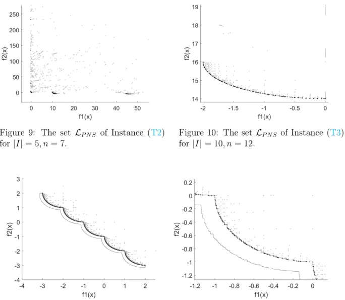
In Figures 9, 10 and 11 we show our results in the image space. As the set LP N S is
similar for all versions of MOMIXand choices of the branching rule within one test instance, we present only the results for MOMIX with (br2) within the figures. In black we plot the points of LP N S. The gray points are the images of the feasible points, i.e., the upper
bounds, computed along the algorithm. The parameter for the set from Theorem 3.13
applied to (T4) with kc = 2 and |I| = 1 is Lδ = 0.1√2. Hence, the set described by
S
z∈LP N S({z−Lδe}+R
m
+) is just a rough lower bound of the nondominated set. From a
practical point of view, in all our test runs, the points from the lists LP N S deliver a good
approximation of the nondominated sets.
Figure 9: The set LP N S of Instance (T2)
for |I|= 5, n = 7.
Figure 10: The set LP N S of Instance (T3)
for |I|= 10, n= 12.
Figure 11: The setLP N S of Instance (T4) for|I|= 1, n− |I|= 2 and the boundary of the
set from Theorem 3.13, Lδ= 0.1√2. Right picture shows a detail of the left one.
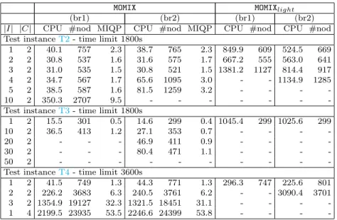
The numerical results on all instances are shown in Table 1. In the first two columns we report the number of integer (|I|) and the number of continuous variables (|C|) for each instance. For both, MOMIX and MOMIXlight, we report the total computational time
For MOMIX we additionally report the total time needed by Gurobi to address the single-objective mixed integer quadratic problems (MIQP). Failures, i.e., instances for which the time limit was exceeded, are marked with “-”.
MOMIX MOMIXlight
(br1) (br2) (br1) (br2)
|I| |C| CPU #nod MIQP CPU #nod MIQP CPU #nod CPU #nod Test instanceT2- time limit 1800s
1 2 40.1 757 2.3 38.7 765 2.3 849.9 609 524.5 669 2 2 30.8 537 1.6 31.6 575 1.7 667.2 555 563.0 641 3 2 31.0 535 1.5 30.8 521 1.5 1381.2 1127 814.4 917 4 2 34.7 567 1.7 65.6 1095 3.0 - - 1134.9 1285 5 2 38.5 587 1.6 81.5 1259 3.2 - - - -10 2 350.3 2707 9.5 - - -
-Test instanceT3- time limit 1800s
1 2 15.5 301 0.5 14.6 299 0.4 1045.4 299 1025.6 299 10 2 36.5 413 1.2 27.1 353 0.7 - - -
-20 2 - - - 46.9 411 0.9 - - -
-30 2 - - - 80.4 471 1.1 - - -
-50 2 - - -
-Test instanceT4- time limit 3600s
1 2 41.5 749 1.3 44.3 771 1.3 296.3 747 225.6 801 2 2 226.2 3683 6.3 240.5 3761 6.2 - - 3090.4 3701 3 2 1354.9 19127 32.3 1321.5 18451 31.1 - - - -1 4 2199.5 23935 53.5 2246.6 24399 53.8 - - -
-Table 1: Numerical results for test instances (T2), (T3) and (T4).
We observe that MOMIX outperforms MOMIXlight on all test instances. MOMIX is able
to solve a higher number of instances within the time limit. This seems to indicate that the improved lower bounding procedure of MOMIX and the effort in solving single-objective mixed integer convex problems pays off. We notice that the time Gurobi needs to address the single-objective mixed integer subproblems is a small percentage of the whole computational time. By using the MATLAB profiler on our code we got that the bottleneck in our implementation isfmincon: Most of the CPU time was spent to solve the single-objective continuous convex problems. In fact, for high dimensional test instances
fmincon was not able to solve some of the single-objective continuous convex problems. This was the case for, e.g., Instance (T3) with|I|= 50. Note thatfminconcan be replaced by any solver for convex problems within both MOMIX and MOMIXlight.
Regarding the two branching rules, we can notice some differences as soon as the dimension of the instances grows.
4.3
Results on a triobjective instance
Our implementation of MOMIX and MOMIXlight can handle instances of (MOMIC) with a
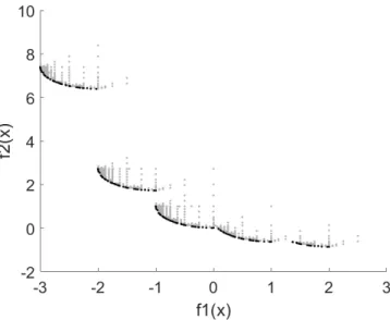
general number of objective functions m ≥ 2. In the following, we present the results obtained by applying MOMIX with branching rule (br2).
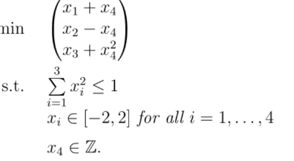
Test instance 4.5 We consider the triobjective mixed integer instance min x1+x4 x2−x4 x3+x24 s.t. 3 P i=1 x2 i ≤1 xi ∈[−2,2] for all i= 1, . . . ,4 x4 ∈Z. (T5)
We set δ = 0.5 in MOMIX. In order to detect LS, the cover of the efficient set of
Problem (T5), MOMIX needed to explore 1237 nodes. This was done within 190 seconds CPU time.
In Figure 12 the points in LP N S are plotted in black, giving an approximation of the
nondominated set of Problem (T5). In gray we plot the images of the feasible points computed along the algorithm.
Figure 12: The set LP N S for Problem (T5) from two different perspectives.
4.4
Results on a convex instance
As a further example, we report the results obtained applying MOMIXlight with branching
rule (br1) on the following non-quadratic instance:
Test instance 4.6 min x1 +x3 x2+ exp(−x3) s.t. x21+x22 ≤1 xi ∈[−2,2] for all i= 1, . . . ,3 x3 ∈Z (T6)
As already mentioned at the beginning of the section, in our implementation of MOMIX
we use GUROBI [19] as mixed integer quadratic solver and we did not include any other solver within it. Therefore, in order to solve Problem (T6) we applied MOMIXlight setting
δ = 0.1. MOMIXlight was able to detect LS by addressing 1105 nodes within 20 seconds
CPU time. In Figure 13, we plot the obtained approximation of the nondominated set of Problem (T6).
Figure 13: The set LP N S of Problem (T6) obtained by MOMIXlight.
Assume that Problem (T6) is solved by using theε-constraint method. Theε-constraint scalarization of (T6) for some ε∈Ris then defined by
min f1(x) =x1+x3 s.t. f2(x) =x2+ exp(−x3)≤ε x21+x22 ≤1 xi ∈[−2,2] for alli= 1, . . . ,3 x3 ∈Z. (7)
Considering the gap in the nondominated set of (T6) (see Figure 13), we have that solving Problem (7) for all values ε in the interval [3,6] would lead to the same solution. The significant values for ε are only those in the intervals [−1,3] and [6,7.5]. Clearly, the significant intervals are not known in advance and this is a big issue when applying the
ε-constraint method on (MOMIC), as the nondominated set of a multiobjective mixed integer convex problem may have huge gaps.
5
Conclusions
In this paper we devised the first deterministic algorithm for solving multiobjective mixed integer convex programming problems. The method is based on linear outer approxima-tions of the image set. We first build linear outer approximaapproxima-tions of the convex relaxation
of the problem by adaptively computing hyperplanes considering some meaningful local upper bounds. Then, in case we want to improve our lower bound, we compute additional hyperplanes that outer approximate the convex hull of the true image set. This is again done in an adaptive way, taking into account specific local upper bounds. The local upper bound sets are updated as soon as a new upper bound is found and are used both to have a pruning criterion and to approximate the dominated set. Theoretical results related to the correctness of our algorithm are provided. Numerical examples on both, biobjec-tive and triobjecbiobjec-tive, instances show the ability of our procedure to detect nondominated points of multiobjective mixed integer convex programming problems. We also explored the possibility of using two different branching rules.
6
Acknowledgments
The first author acknowledges support within the DAAD scholarship No 57440915. She further acknowledges support within the project No RP1181641D22304F which has re-ceived funding from Sapienza, University of Rome. The third author thanks the Carl-Zeiss-Stiftung and the DFG-founded Research Training Group 1567 for financial support. The work of the fourth author is funded by the Deutsche Forschungsgemeinschaft under grant No. EI 821/4.
References
[1] P. Belotti, C. Kirches, S. Leyffer, J. Linderoth, J. Luedtke, and A. Mahajan. Mixed-integer nonlinear optimization. Acta Numerica, 22:1–131, 2013.
[2] N. Boland, H. Charkhgard, and M. Savelsbergh. A criterion space search algorithm for biobjective integer programming: The balanced box method. INFORMS J. Comput., 27(4):735–754, 2015.
[3] N. Boland, H. Charkhgard, and M. Savelsbergh. The l-shape search method for triobjective integer programming. Math. Program. Comput., 8(2):217–251, 2016. [4] N. Boland, H. Charkhgard, and M. Savelsbergh. A new method for optimizing a linear
function over the efficient set of a multiobjective integer program. Eur. J. Oper. Res., 260(3):904–919, 2017.
[5] N. Boland, H. Charkhgard, and M. Savelsbergh. The quadrant shrinking method: A simple and efficient algorithm for solving tri-objective integer programs. Eur. J. Oper. Res., 260(3):873–885, 2017.
[6] N. Boland, A. C. Eberhard, F. Engineer, and A. Tsoukalas. A new approach to the feasibility pump in mixed integer programming. SIAM J. Optim., 22(3):831–861, 2012.
[7] P. Bonami, G. Cornu´ejols, A. Lodi, and F. Margot. A feasibility pump for mixed integer nonlinear programs. Math. Program., 119(2):331–352, 2009.
[8] R. S. Burachik, C. Y. Kaya, and M. M. Rizvi. Algorithms for generating pareto fronts of multi-objective integer and mixed-integer programming problems. arXiv:1903.07041v1.
[9] R. S. Burachik, C. Y. Kaya, and M. M. Rizvi. A new scalarization technique and new algorithms to generate pareto fronts. SIAM J. Optim., 27(2):1010–1034, 2017. [10] V. Cacchiani and C. D’Ambrosio. A branch-and-bound based heuristic algorithm for
convex multi-objective minlps. Eur. J. Oper. Res., 260(3):920–933, 2017.
[11] M. De Santis, S. Lucidi, and F. Rinaldi. A new class of functions for measuring solution integrality in the feasibility pump approach. SIAM J. Optim., 23(3):1575– 1606, 2013.
[12] M. Ehrgott and X. Gandibleux. Bound sets for biobjective combinatorial optimization problems. Comput. Oper. Res., 34:2674–2694, 2007.
[13] M. Ehrgott, L. Shao, and A. Sch¨obel. An approximation algorithm for convex multi-objective programming problems. J. Global Optim., 50(3):397–416, 2011.
[14] M. Ehrgott, C. Waters, R. Kasimbeyli, and O. Ustun. Multiobjective programming and multiattribute utility functions in portfolio optimization. INFOR Inf. Syst. Oper. Res., 47(1):31–42, 2009.
[15] M. Fischetti, F. Glover, and A. Lodi. The feasibility pump. Math. Program., 104(1):91–104, 2005.
[16] B. Geißler, A. Morsi, L. Schewe, and M. Schmidt. Penalty alternating direction methods for mixed-integer optimization: A new view on feasibility pumps. SIAM J. Optim., 27(3):1611–1636, 2017.
[17] A. Gleixner, M. Bastubbe, L. Eifler, T. Gally, G. Gamrath, R. L. Gottwald, G. Hendel, C. Hojny, T. Koch, M. E. L¨ubbecke, S. J. Maher, M. Miltenberger, B. M¨uller, M. E. Pfetsch, C. Puchert, D. Rehfeldt, F. Schl¨osser, C. Schubert, F. Serrano, Y. Shinano, J. M. Viernickel, M. Walter, F. Wegscheider, J. T. Witt, and J. Witzig. The SCIP Optimization Suite 6.0. ZIB-Report 18-26, Zuse Institute Berlin, July 2018.
[18] O. G¨unl¨uk, J. Lee, and R. Weismantel. Minlp strengthening for separable convex quadratic transportation-cost ufl. IBM Res. Report, pages 1–16, 2007.
[19] LLC Gurobi Optimization. Gurobi optimizer reference manual, 2018. [20] J. Jahn. Vector Optimization. Springer, 2009.
[21] K. Klamroth, R. Lacour, and D. Vanderpooten. On the representation of the search region in multi-objective optimization. Eur. J. Oper. Res., 245(3):767–778, 2015. [22] A. L¨ohne, B. Rudloff, and F. Ulus. Primal and dual approximation algorithms for
[23] G. Mavrotas. Effective implementation of theε-constraint method in multi-objective mathematical programming problems. Appl. Math. Comput., 213(2):455–465, 2009. [24] G. Mavrotas and D. Diakoulaki. A branch and bound algorithm for mixed zero-one
multiple objective linear programming. Eur. J. Oper. Res., 107(3):530–541, 1998. [25] G. Mavrotas and D. Diakoulaki. Multi-criteria branch and bound: A vector
maxi-mization algorithm for mixed 0-1 multiple objective linear programming. Appl. Math. Comput., 171(1):53–71, 2005.
[26] J. Niebling and G. Eichfelder. A branch-and-bound-based algorithm for nonconvex multiobjective optimization. SIAM J. Optim., 29(1):794–821, 2019.
[27] Julia Niebling and Gabriele Eichfelder. A branch-and-bound algorithm for bi-objective problems. In Proceedings of the XIII Global Optimization Workshop GOW’16, pages 57–60, 2016.
[28] Y. Peng and L. Yu. Multiple criteria decision making in emergency management.
Comput. Oper. Res., 42:1–2, 2014.
[29] F. Sourd and O. Spanjaard. A multiobjective branch-and-bound framework: Applica-tion to the biobjective spanning tree problem. INFORMS J. Comput., 20(3):472–484, 2008.
[30] P. Xidonas, G. Mavrotas, and J. Psarras. Equity portfolio construction and selection using multiobjective mathematical programming. J. Global Optim., 47(2):185–209, 2010.