A SPARSE MARKOV CHAIN APPROXIMATION OF LQ-TYPE STOCHASTIC CONTROL PROBLEMS
RALF BANISCH∗ AND CARSTEN HARTMANN†
Abstract. We propose a novel Galerkin discretization scheme for stochastic optimal control problems on an indefinite time horizon. The control problems are linear-quadratic in the controls, but possibly nonlinear in the state variables, and the discretization is based on the fact that problems of this kind admit a dual formulation in terms of linear boundary value problems. We show that the discretized linear problem is dual to a Markov decision problem, prove anL2 error bound for the general scheme and discuss the sparse discretization using a basis of so-called committor functions as a special case; the latter is particularly suited when the dynamics are metastable, e.g., when controlling biomolecular systems. We illustrate the method with several numerical examples, one being the optimal control of Alanine dipeptide to its helical conformation.
1. Introduction. A large body of literature, going back to the seminal work by Kramers [25] in the late 1930ies, is concerned with the question: How well can a continuous diffusion in a multi-well energy landscape be approximated by a Markov jump process (MJP) in the regime of low temperatures?. Qualitatively, the approxi-mation should be good if the system under consideration is metastable, in which case the process stays in the neighbourhood of the potential energy minima for a long time and occasionally makes rapid transitions (jumps) between the wells. These metastable regions then become the states of the MJP, and the jump rates are determined by the frequency of the transitions (see, e.g., [32, 35]).
In this article we consider the approximation of optimal control problems with nonlinear diffusive dynamics by discrete Markov decision problems. This situation is more complicated than in Kramers’ case, for one has to approximate the dynamics as well as the corresponding cost functional and the resulting control forces. The difficulty comes from the fact that dynamics enter as a constraint in the optimization of the cost functional, which makes the problem nonlinear, because the controls become a priori unknown functions of the state variables. Specifically, we consider reversible diffusions on an unbounded domain, with a cost functional that is linear-quadratic in the controls, but possibly nonlinear in the state variables, and that is defined up to some random stopping time. The control problem admits a dual formulation in form of linear boundary value problem that is amenable to a discretization by standard means (cf. [37, 48]). Problems of this kind appear relevant in various applications, including molecular dynamics [41], material science [42] or quantum computing [33], to mention just a few. We propose a Markov chain approximation (MCA) that is based on a Galerkin discretization the underlying dynamic programming equations, with basis functions that cover the metastable sets of the dynamics. The discretized problem can be interpreted as a Markov decision problem where the dynamics is given by a continuous-time Markov process on the metastabe sets (so-calledcore sets). As these core sets are not assumed to cover the state space, the method is sparse and meshless and hence can be applied to large-scale problems.
MCA are a versatile tool to approximate stochastic control problems. Going back to Kushner [26], the idea of MCA is to approximate the spatially discretized dynamics by a Markov chain and reformulate the underlying continuous control problem as
∗Freie Universit¨at Berlin, Institut f¨ur Mathematik, Arnimallee 6, 14195 Berlin, Germany
([email protected]). This author holds a scholarship from the Berlin Mathematical School.
†Corresponding author. Freie Universit¨at Berlin, Institut f¨ur Mathematik, Arnimallee 6, 14195
Berlin, Germany ([email protected]). 1
a control problem for the approximating chain. For a spatial discretization with uniform grid, the MCA amounts to a finite-difference discretization of the dynamic programming equation [28, 30]. Recent advances in MCA include collocation-based schemes with radial basis functions [24], finite volume approximations [46], switched systems and jump diffusions [40], or multi-player differential games [39].
The MCA that we propose here for the indefinite time-horizon case is based on a meshless Galerkin discretization of the dual problem. This discretization is standard in that it shares features with related Galerkin methods for linear elliptic equations (see, e.g., [1, 47]), however it is novel in that it preserves the particular structure of the reversible dynamics and the duality of the underlying Markov decision problem when the basis functions form a partition of unity. Related problems with indefinite time-horizon using grid-based techniques have been studied in [22, 43, 27]; cf. also [4] for a (non-Markovian) finite element method. For meshless discretizations of the parabolic dynamic programming equation of finite time-horizon problems we refer to, e.g., [9, 24]; related ideas for the first-order dynamic programing equations of deterministic control have been used in [3, 8].
A simple paradigm. As an introductory example consider the one-dimensional diffusion process (Xt)t≥0 satisfying the Itˆo stochastic differential equation
dXtu= (ut− ∇V(Xtu))dt+
√
2dBt, t≥0 (1.1)
where Bt is standard Brownian motion, >0 is noise intensity, called temperature
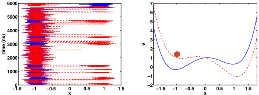
in the following, V is the bistable potential energy shown in Figure 1.1, and uis a bounded measurable function, thecontrol. Let us suppose that the control task is to force the particle in the left well to reach the right well in minimum time τ. When u= 0 and noise is low, the average transition timeE[τ] is exponentially large in the energy barrier ∆V between the wells, and we can decrease the barrier by tilting the potential according to V(x) 7→V(x)−ux. A controller will then seek to minimize the average transition time by tilting the potential without applying too much force, which leads to a quadratic cost functional of the form [37]
J(u) =E τ+γ Z τ 0 |ut|2dt , γ >0,
that must be minimized over a set of admissible (e.g. adapted) control strategies, subject to the stochastic dynamics (1.1). (Hereγ >0 is an adjustable parameter.)
In this paper we deal with the question how to solve optimal control problems of the above form beyond simple one-dimensional examples. The typical application that we have in mind is molecular dynamics that is both high-dimensional and displays vastly different time scales. This defines the basic requirements of the numerical method: it must handle problems with large state space dimension and it must be able to capture the relevant processes of the dynamics, typically the slowest degrees of freedom in the system. For moderate controls, and if the temperature is small compared to the energy barrier, the dynamics in the above example basically consists of rare jumps between the potential wells, with the jump rate being controlled by u. An efficient discretization would be one that resolves only the jumps between the wells by a 2-state Markov jump process with adjustable jump rates, according to the value of the control (cf. [12, 35]). It is known (see [16]) that control problems of the above form can be transformed into a dual linear boundary value problem that can be approximated by an MJP on the metastable sets. The discretized linear
−01.5 −1 −0.5 0 0.5 1 1.5 1000 2000 3000 4000 5000 6000 x time (ns)
Fig. 1.1: Two typical realizations of the bistable system (1.1), with and without tilting (left panel). The corresponding potential energies are shown in the right panel.
problem turns out to be dual to a Markov decision problem and thus represents the natural Markovian discretization of the original stochastic control problem. The discretization is meshless, in that the number of states of the Markov model does not scale exponentially with the dimension of the continuous state space, hence the method avoids the curse of dimensionality of most grid-based schemes.
Organization of the article. The rest of the paper is organised as follows: In section 2 we introduce the class of optimal control problems studied and state the duality between optimal control and sampling for both continuous SDEs and MJPs. In section 3, the Galerkin projection method is introduced, and some results about the approximation error are discussed. We also give a stochastic interpretation of the discretized linear equation in terms of Elber’s milestoning process [14]. Finally, we construct sampling estimators. Section 3 is the core parts of the paper and con-tains new results, including the meshless Galerkin algorithm and an estimate of the discretization error inL2. In section 4, we discuss numerical examples.
1.1. Elementary notation and assumptions. We implement the following notation and standing assumptions that will be used throughout the paper.
Dynamics. Let S = Rd and consider the potential energy function V: S →
R, that we assume to be two times continuously differentiable and bounded from
below. Further assume that V(x) is polynomially growing at infinity like |x|2k for
some positive integerk. We consider the processXt∈ S solving
dXu
t = (ut− ∇V(Xtu))dt+
√
2dBt, t≥0, (1.2)
whereBt∈Rdisd-dimensional Brownian motion under a probability measureP, and
u: [0,∞)→U ⊂Rd is a time dependent measurable and bounded function.
Reversibility and invariant measure. For test functions ϕ:S →Rthat are
two times continuously differentiable, the infinitesimal generator of the uncontrolled processXt=Xt0 is defined as the second-order differential operator
Lϕ=∆ϕ− ∇V · ∇ϕ . Define
dµ(x) = exp(−−1V(x))dx 3
to be the Boltzmann measure at temperature > 0. Without loss of generality, we assume thatµis normalized, so thatµ(S) = 1. For the subsequent analysis it will be convenient to think ofLas an operator acting on a suitable subspace of
L2(S, µ) = φ:S →R: Z S |φ(x)|2dµ(x)<∞ , that is a weighted Hilbert space equipped with the scalar product
hv, wiµ=
Z
S
v(x)w(x)dµ(x).
It can be readily seen thatLis symmetric with respect to the weighted scalar product, hLv, wiµ=hv, Lwiµ ,
which implies thatXtis reversible with respect to the Boltzmann measureµ.
More-over, by the above assumptions on the potential energy function, µ is the unique invariant measure of the processXtand satisfies
Z S (Lψ)dµ= Z S ψ(L1)dµ= 0 for all test functionsψ∈L2(S, µ); see [29] for details.
Quadratic cost criterion. We now introduce the cost criterion that the con-troller choosing u in (1.2) seeks to minimize. To this end let A ⊂ S be a closed bounded subset of positive measure µ(A) > 0 with smooth (at least C3) boundary ∂Aand callτA<∞the random stopping time
τA= inf{t >0 :Xt∈∂A}.
We define the cost functional J(u) =E Z τA 0 f(Xtu) + 1 4|ut| 2 dt , (1.3)
where f: S → R, called running cost, is any bounded nonnegative function with
bounded first derivative; the factor 1/4 in the penalization term is merely conventional. Cost functionals of this form are called indefinite time horizon cost, because the terminal time τA is random. We will sometimes need the conditioned variant of
the above cost functional:
J(u;x) =Ex Z τA 0 f(Xtu) + 1 4|ut| 2 dt . (1.4)
HereEx[·] =E[·|X0=x] is a shorthand for the expectation over all realizations ofXt
starting atX0=x, i.e. the expectation with respect toP conditional onX0=x. We useJ to denote both unconditional and conditional cost functionals; it should always be clear from the context, which one is meant.
Admissible control strategies. We call a control strategyu= (ut)t≥0 admis-sible if it is adapted to the filtration generated byBt, i.e., ifut depends only on the
history of the Brownian motion up to timet, and if the equation forXu
t has a unique
strong solution. The set of admissible strategies is denoted byA.
Even thoughutmay depend on the entire past history of the process up to time
t, it turns out that optimal strategies are Markovian, i.e., they depend only on the current state of the system at timet. In our case, in which the costs are accumulated up to a random stopping timeτA, the optimal strategies are of the form
ut=α(Xtu)
for some function α: S → Rd. Hence the optimal controls are time-homogeneous
feedback policies, depending only on the current stateXu
t, but not ont.
2. Optimal control and logarithmic transformation. In this section we es-tablish a connection between controlled diffusions and certain path sampling problems, the latter are associated with a linear boundary value partial differential equation (PDE) that can be discretized by standard numerical techniques for PDEs or Monte-Carlo. The duality between optimal control and path sampling goes back to Wendel Fleming and co-workers (see, e.g, [15]) and is based on a logarithmic transformation of the value function (see also [16, Sec. VI] and the references therein)
W(x) = min
u∈AJ(u;x). (2.1)
2.1. Duality between control and path sampling for diffusions. Our sim-ple derivation of the duality between path sampling optimal control will be based on the Hamilton-Jacobi-Bellman equations of optimal control. To this end, we recall the dynamic programming principle for optimal control problems of the form (1.2)–(1.3) that we adapt from [16, Secs. VI.3–5] and that we state without proof.
Theorem 2.1. Let W ∈C2(S \A)∩C(∂A)be the solution of
min c∈Rd (L+c· ∇)W(x) +f +1 4|c| 2 = 0, x∈ S \A W(x) = 0, x∈∂A . (2.2) Then W(x) = min u∈AJ(u;x)
where the minimizeru∗= argminJ(u)is unique and given by the feedback law
ut=−2∇W(Xtu). (2.3)
Before we proceed with the derivation of the dual sampling problem, we shall briefly discuss some of the consequences of the dynamic programming approach. Equation (2.2) is the Hamilton-Jacobi-Bellman (HJB) equation, also calleddynamic programming equation associated with the following optimal control task:
min u∈AJ(u) s.t. dX u t = (ut− ∇V(Xtu))dt+ √ 2dBt. 5
The function W(x) is calledvalue function or optimal cost-to-go. Using the fact that optimal control is the gradient of two times the value function, the optimally controlled processX∗
t solves the SDE
dXt∗=−∇U(Xt∗)dt+
√
2dBt. (2.4)
with the new potential
U(x) =V(x) + 2W(x). Note that X∗
t is reversible with respect to a tilted Boltzmann distribution having
the density ρ∗ = exp(−U/). The reversibility follows from the fact that the value function does not depend on t, which would not be the case if the terminal timeτA
were a deterministic stopping time rather than a first exit time.1
Logarithmic transformation and Feynman-Kac formula (part I). The approach that is pursued in this article is to discretize the HJB equation by first removing the nonlinearity by a logarithmic transformation of the value function. Let φ(x) = exp(−−1W(x)). (2.5) It follows by chain rule that
Lφ
φ =−LW +|∇W|
2, φ6= 0, (2.6)
which, together with the relation −|∇W|2= min c∈Rm c· ∇W+1 4|c| 2 ,
implies that (2.2) is equivalent to the linear boundary value problem L−−1f
φ(x) = 0, x∈ S \A
φ(x) = 1, x∈∂A . (2.7)
By the above assumptions and the strong maximum principle for elliptic PDEs it follows that (2.7) has a classical solution φ∈ C2(S \A)∩C(∂A) that is uniformly bounded away from zero. The latter, together with (2.5)–(2.6), implies existence and uniqueness of classical solutions of that the dynamic programming equation (2.2) and hence smoothness of the value function.
Now, by the Feynman-Kac theorem [31, Thm. 8.2.1], the linear boundary value problem has an interpretation in terms of a sampling problem. The solution (2.7) can be expressed as the conditional expectation
φ(x) =Ex exp −1 Z τA 0 f(Xt)ds (2.8) over all realizations of the following SDE onS:
dXt=−∇V(Xt)dt+
√
2dBt, X0=x . (2.9)
1For finite time-horizon control problems the value function depends on the timeτ
A−tremaining
until the terminal timeτA.
2.2. Duality between control and path sampling for jump processes. In the last section, we have established a connection between an optimal control problem and sampling of a continuous path observableφ(x). In this section, we will repeat the same construction for MJP, however, in reverse order: starting from a path observable for a MJP, we derive the dual optimal control using a logarithmic transformation.
Let ( ˆXt)t≥0be a MJP on the discrete state space ˆS={1, . . . , n}with infinitesimal generatorG∈Rn×n. (For simplicity, we assume that ˆS is finite.) The entries of the
generator matrixGsatisfy
Gij≥0 fori6=j and Gii =− X j6=i
Gij,
where the off-diagonal entries ofGare the jump rates between the statesi andj.
Logarithmic transformation and Feynman-Kac formula (part II). In accordance with the previous subsection let ˆf : ˆS →Rbe nonnegative and define the
stopping timeτA= inf{t >0 : ˆXt∈A}to be the first hitting time of a subsetA⊂Sˆ.
As before we introduce a function ˆ φ(i) =Ei exp −1 Z τA 0 ˆ f( ˆXs)ds ,
withEi[·] =E[·|Xˆ0=i] being the conditional expectation over the realizations of ˆXt
starting at ˆX0 =i. We have the following lemma that is the exact analogue of the Feynman-Kac formula for diffusions for the case of an MJP (see [17]).
Lemma 2.2. The functionφ(i)ˆ solves the linear boundary value problem
X j∈Sˆ Gijφˆ(i)−−1fˆ(i) ˆφ(i) = 0, i∈S \ˆ A ˆ φ(i) = 1, i∈A . (2.10)
Now, in one-to-one correspondence with the log transformation procedure in the diffusion case, the function
ˆ
W =−log ˆφ
can be interpreted as the value function of an optimal control problem for the MJP ( ˆXt)t≥0. The derivation of the dual optimal control problem goes back to [38], and we repeat it here in condensed form for the reader’s convenience (see also [16, Sec. VI.9]): First of all note that ˆW satisfies the equation
exp( ˆW /)Gexp(−W /)ˆ −−1fˆ= 0, i∈S \ˆ A ˆ
W(i) = 0, i∈A . and define a new generator matrix by
Gv = (Gvij)i,j∈Sˆ, Gvij =
Gijv(j)
v(i) , (2.11)
withv(i)>0 for alli∈Sˆ. The exponential term in the above equation for ˆW can be recast as (Gφ)(i)ˆ ˆ φ(i) = −1min v>0{−(G vWˆ)(i) +kv(i)} 7
where we have introduced the shorthand
kv(i) =(Gv(logv))(i)−(Gv)(i) v(i) ,
and used the identity miny∈R{e−y+ay}=a−alogafor a >0. As a consequence, (2.10) is equivalent (i.e. dual) to
min
v>0
n
(GvWˆ)(i) +kv(i) + ˆf(i)o= 0, i∈S \ˆ A ˆ
W(i) = 0, i∈A .
(2.12)
which is the dynamic programming equation of a Markov decision problem, i.e. an optimal control problem for an MJP (e.g. see [16, Sec. VI.9]): Minimize
ˆ J(v) =E Z τA 0 n ˆ f( ˆXsv) +kv( ˆXsv) o ds (2.13)
over all controlsv >0 and subject to the constraint that the process ( ˆXv
t)t≥0is gen-erated byGv. It readily follows from the derivation of (2.12) that the minimizer exists
and is given by v∗(i) = ˆφ(i). The next lemma records some important properties of the controlled Markov jump process with generator Gv and the corresponding cost functional (2.13).
Lemma 2.3. Let Gv andkv be defined as above.
(i) Let G be reversible with unique stationary distribution π. Then πv(i) =
Z−1
v v2(i)π(i), with Zv an appropriate normalization constant, is the unique
probability distribution such thatGv is reversible with stationary distribution
πv.
(ii) LetPˆ denote the probability measure on the space of trajectories generated by ˆ
Xt with initial conditionXˆ0 =i, and let Qˆ be the corresponding probability measure generated by Xˆv
t with the same initial conditionXˆ0v =i. Then Qˆ is absolutely continuous with respect toPˆ and the expected value of the running costkv is the Kullback-Leibler (KL) divergence betweenQˆ andPˆ, i.e.,
EQˆ Z τA 0 kv( ˆXv s)ds = Z logd ˆ Q dPˆd ˆ Q
whereEQˆ[. . .]is the expectation over all realizations ofXˆtvstarting atXˆ0v=i. Proof. We first show (i). By assumption we haveπ(i)Gij =π(j)Gji. Now, letπv
be such thatπv(i)Gv
ij =πv(j)Gvji. We will show thatπv has the proposed form:
πv(i)Gvij= v(j) v(i) πv(i) π(i) π(i)Gij = v(j) v(i) πv(i) π(i)π(j)Gji= v2(j) v2(i) π(j) π(i) πv(i) πv(j)π v(j)Gv ji
But sinceπv(i)Gv
ij =πv(j)Gvji, we must have
πv(j)
π(j)v2(j)=
πv(i)
π(i)v2(i) ∀i6=j. This can only be true if the quantityZ−1
v = πv(i)
π(i)v2(i) is independent of i. This gives πv(j) = Z−1
v v2(j)π(j) as desired. The constant Zv is uniquely determined by the
requirement thatπv be normalized. Finally, from reversibility it follows directly that
πv is also a stationary distribution ofGv.
To show (ii), note that the running costkv(i) can be written as
kv(i) =X j6=i Gij v(j) v(i) logv(j) v(i) −1 + 1 , (2.14)
which is the KL divergence between ˆQ and ˆP (see [10, Sec. 3.1.4]). The absolute continuity between ˆQ and ˆP simply follows from the fact thatv in the definition of Gv was required to be component-wise strictly positive.
Remark 1. To reveal further similarities between (1.2)–(1.3) and the correspond-ing Markov decision problem, note that the quadratic penalization term in (1.3) equals the KL divergence between the reference measureP of the uncontrolled diffusion (2.9) and the probability measureQ of the controlled process (1.2), as can be shown using Girsanov’s theorem [31, Thm. 8.6.8]. It holds that (cf. [20, 18]):
EQ 1 4 Z τA 0 |us|2ds = Z logdQ dPdQ .
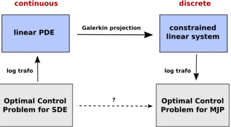
3. Discretization: Galerkin projection point of view. In this section we will develop a discretization for optimal control problems of the type discussed in Section 2 using the method of logarithmic transformations. The discretization will approximate the continuous control problem with a control problem for a Markov jump process on finite state space. Our strategy is outlined in Figure 3.1.
Optimal Control Problem for SDE
Optimal Control Problem for MJP
continuous discrete
linear PDE constrained
linear system
log trafo log trafo
Galerkin projection
?
Fig. 3.1: Discretization of continuous control problems via a logarithmic transform.
In the first part of this section, we will develop the Galerkin projection for general subspaces and obtain some control of the discretization error. To refine this control, we specify the subspace D we project onto. As the state space is unbounded and possibly high-dimensional, a grid-based discretization is prohibitive. Here we suggest a meshless discretization based on an incomplete partition of state space into so called core sets, that are the metastable regions of the uncontrolled dynamics. We will prove an error bound which gives us detailed control over the discretization error, even if very few basis functions are used. We should mention that clearly other choices
are possible, such as radial basis functions [47] or moving least-squares [1], but for metastable systems like in molecular dynamics or chemical reaction kinetics using core sets and the associated basis of committor functions is beneficial.
In the second part of this section, we will develop the stochastic interpretation of the resulting matrix equation as the backward Kolmogorov equation of a MJP, which enables us to identify the discrete control problem for the MJP, as it was developed in Section 2. We will study the resulting discrete control problem and make a connection to Transition Path Theory [45] and core set Markov state models (MSM) [36].
3.1. Galerkin projection of the Dirichlet problem. As discussed above, we consider the boundary value problem
L−−1f
φ(x) = 0, x∈ S \A
φ(x) = 1, x∈∂A . (3.1)
withLandf as given above. We declare thatφ|A= 1, so that the domain of φisS.
Following standard references (e.g. [6]) we construct a Galerkin projection of (3.1). For this purpose, we introduce the L2-based Sobolev space H1 with norm kφkH1 =k∇uk2µ+kuk2µ and the Hilbert spacesV ={ψ∈L2(S, µ),kψkH1<∞}and V0={ψ∈V, ψ|∂A= 0}. We further define the symmetric and positive bilinear form
B:V ×V →R, B(φ, ψ) =−1hf φ, ψiµ+h∇φ,∇ψiµ.
Now ifφis a solution of (3.1), then it also solves the weak problem
B(φ, ψ) = 0 ∀ψ∈V0. (3.2)
AGalerkin solutionφˆis now any function satisfying
B( ˆφ,ψ) = 0ˆ ∀ψˆ∈D0, (3.3) withD0being a suitable finite dimensional subspaceV0. Specifically, we choose basis functionsχ1, . . . , χn+1 with the following properties:
(S1) The functionsχi:S →Rare in V.
(S2) Theχi form a partition of unity, that isPni=1+1χi=1. (S3) Theχi satisfyχn+1|A= 1 and χi|A= 0 fori∈ {1, . . . , n}.
All elements ofD0:= lin{χ1, . . . , χn}will satisfy homogeneous Dirichlet boundary
conditions in (3.1), and we will sometimes write D := χn+1⊕D0 and think of the Galerkin solution ˆφas an element inD. Now define the matrices
Fij= hχi, f χjiµ hχi,1iµ , Kij =− h∇χi,∇χjiµ hχi,1iµ . Setting ˆφ=P
iφˆiχi, the weak form (3.3) becomes a matrix equation for the unknown
coefficients ˆφi: n+1 X j=1 Kij−−1Fij ˆ φj= 0, i∈ {1, . . . , n} ˆ φn+1= 1, (3.4) 10
which is the discretization of (3.1).
In order control the discretization error of the Galerkin method, we choose a norm k · konV and introduce the two error measures:
1. The Galerkin error ε = kφ−φˆk, i.e. the difference between original and Galerkin solution measured ink · k.
2. Thebest approximation errorε0= infψˆ∈Dkφ−ψˆk, i.e. the minimal difference between the solutionφand any element ˆψ∈D.
In order to obtain full control over the discretization error, we need bounds onε, and we will get them by first obtaining a bound on the performancep:=ε/ε0 and then a bound on ε0. The latter will depend on the choice of subspace D. For the
former, standard estimates assume the followingk · k-dependent properties ofA: (i) Boundedness: B(φ, ψ)≤α1kφkkψkfor some α1>0
(ii) Ellipticity: for allφ∈V holdsB(φ, φ)≥α2kφkfor someα2>0. If both (i) and (ii) hold, C´ea’s lemma states that p≤ α1
α2, see e.g. [6]. For the energy norm kφk2
B := B(φ, φ) we have α1 =α2 = 1 and therefore p = 1, thus the Galerkin solution ˆφis the best-approximation toφin the energy norm.
Performance bound. The next two statements give a bound onpif errors are measured in theL2-norm. In this case,B(·,·) is still elliptic but possibly unbounded. Later in this section, we will specify the bound onε0for a specific Galerkin basis.
Theorem 3.1. Let B be elliptic. Further let
Q:L2(S, µ)→D 0⊂L2(S, µ), Qw= n X i=1 hχi, wiχi
be the orthogonal projection onto D0. Then
p2= ε ε0 2 ≤1 + 1 α2 2 sup v∈V kQB(1−Q)vk2 µ kvk2 µ
whereB=−1f −Lis the linear operator associated withφ7→ B(·, φ). Proof. In Appendix A.
Remark 2. Note that kQB(1−Q)vkµ ≤ kQBvkµ is always finite even though
B is possibly unbounded sincev∈V ⊂L2(S, µ)andQis the projection onto a finite-dimensional subspace of L2(S, µ).
The bottom line of Theorem 3.1 is that ifB leaves the subspaceDalmost invari-ant, then ˆφis almost the best-approximation ofφink · kµ. The following lemma gives
a more detailed description. In the following, we will writek·k=k·kµfor convenience.
Lemma 3.2. Let Q⊥=1−Qand define
δL:= max k kQ ⊥Lχ kk, δf := max k kQ ⊥−1f χ kk
to be the maximal projection error of the images of theχk’s under Landf. Then
kQBQ⊥k=kQ⊥BQk ≤(δ L+δf) r n m 11
wherem is the smallest eigenvalue ofMˆ.
Proof. The first statement is true sinceAis essentially self-adjoint. For the second statement, first of all
kQ⊥BQk=kQ⊥(−1f−L)Qk ≤ kQ⊥−1f Qk+kQ⊥LQk
holds from the triangle inequality. We now bound the term involvingL. Notice that for ˆφ=P iφˆiχi∈D: kQ⊥Lφˆk=kX i ˆ φiQ⊥Lχik ≤δL X i |φˆi|=δLkφˆk1. Then, with ˆM := (hχi, χjiµ)ij: kQ⊥LQk= sup φ=φ||+φ⊥∈V kQ⊥Lφ ||k kφk ≤φsup||∈D kQ⊥Lφ ||k kφ||k ≤δL sup ˆ φ∈Rn kφˆk1 q hφ,ˆ φˆiM
A similar result holds for the term involvingf. The statement now follows from a standard equivalence between finite-dimensional norms, kφˆk1 ≤√nkφˆk2, and the fact that ˆM is symmetric, which implies thathφ,ˆ φˆiM = ˆφTMˆφˆ≥mφˆTφˆ=mkφˆk22.
To summarize, Theorem 3.1 and Lemma 3.2 give us a formula for the projection performancepwhich states that
p2≤1 + n m (δL+δf)2 α2 2 .
How large or smallδf is will depend on the behaviour off, e.g., iff = const then
δf = 0. Bothδf andδL are always finite even thoughL is possibly unbounded. Best-approximation error bound. We now generalize results [12] on the ap-proximation quality of MSMs for reversible equilibrium diffusions and estimate the best-approximation errorε0for the case that the subspaceDis spanned by committor functions associated with the metastable sets of the dynamics. To this end suppose that the potential V(x) has n+ 1 deep minima x1, . . . , xn+1. Let C1, . . . , Cn+1 be convexcore sets aroundx1, . . . , xn+1and such thatA=Cn+1. We writeC=∪ni=1+1Ci
and T = S \C and introduce τC = inf{t ≥ 0 : Xt ∈ C}. We take χi to be the
committor function associated with the setCi, that is
χi(x) =P(XτC ∈Ci|X0=x). (3.5)
Theseχisatisfy the assumptions (S2)–(S3) and (S1) expect on the core set
bound-aries, which is a set of measure zero. Since we do not have a grid parameter, by which the approximation error can be controlled, standard PDE techniques for boundingε0
fail. Indeed, typically we will have very few basis functions compared to a grid-like discretization. The following theorem gives a bound onε0.
Theorem 3.3. Let Q be the orthogonal projection onto the subspace D spanned
by the committor functions (3.5), and letφbe the solution of (3.1). Then we have
ε0=kQ⊥φkµ≤ kP⊥φkµ+µ(T)1/2κkfk∞+ 2kP⊥φk∞ 12
wherek · k=k · kµ,κ= supx∈TEx[τS\T], andP is the orthogonal projection onto
Vc={v∈L2(S, µ), v|Ci=conston everyCi} ⊂L
2(S, µ), with P⊥ =
1−P. Proof. In Appendix B
In Theorem 3.3, κis the maximum expected time of hitting the metastable set from outside (which is short). Note further thatP⊥φ= 0 on T. The errors kP⊥φkµ
and kP⊥φk
∞ measure how constant the solution φ is on the core sets. Theorem 3.3 suggest the following strategy to minimize ε0: (i) Place a core set Ci in every
metastable region where φ is expected to be almost constant, (ii) place core sets in regions with high invariant density µ in order to minimize µ(T). This strategy requires knowledge of the invariant density µ. Identifying the metastable regions requires additional dynamical information. If this is not available, then a good guess is usually to use the deepest wells ofµ.
Remark 3. Theorem 3.3 together with Theorem 3.1 gives us full control over
the discretization error ε. These error bounds generalize recent results [35, 12] on the approximation quality of the dominant eigenvalues of a reversible diffusion by an MSM to general (bounded, nonnegative) observables.It would of course be nice to have an error estimate also for the value function. In general such an estimate is difficult to get, because of the nonlinear logarithmic transformation W = −logφ involved. However we know that φ and its discrete approximation are both uniformly bounded and bounded away from zero. Hence the logarithmic transformation is uniformly Lip-schitz continuous on its domain, which implies that theL2 error bounds holds for the value function with an additional prefactor given by the Lipschitz constant squared; for a related argument see [19]
3.2. Interpretation in terms of a Markov decision problem. We derive an interpretation of the discretized equation (3.4) in terms of a MJP. We introduce the diagonal matrix Λ with entries Λii=PjFij (zero otherwise) and the full matrix
G=K−−1(F−Λ), and rearrange (3.4) as follows:
n+1 X j=1 Gij−−1Λijφˆj= 0, i∈ {1, . . . , n} ˆ φn+1= 1, (3.6)
This equation can be given a stochastic interpretation. To this end let us in-troduce the vector π ∈ Rn+1 with nonnegative entries πi =hχi,1i and notice that P
iπi= 1 follows immediately from the fact that the basis functionsχi form a
parti-tion of unity, i.e. P
iχi=1. This implies thatπis a probability distribution on the
discrete state space ˆS ={1, . . . , n+ 1}. We summarize properties of the matricesK, F andG:
Lemma 3.4. Let K,G,F andπ be as above.
(i) K is a generator matrix (i.e. K is a real-valued square matrix with row sum zero and positive off-diagonal entries) with stationary distributionπthat satisfies detailed balance
πiKij=πjKji, i, j∈Sˆ
(ii) F ≥0(entry-wise) with πiFij =πjFji for alli, j∈Sˆ.
(iii) Ghas row sum zero and satisfiesπTG= 0andπ
iGij=πjGjifor alli, j∈Sˆ.
(iv) There exists a (possibly-dependent) constant0< C <∞such that Gij ≥0
for all i 6=j if kfk∞ ≤C. In this case equation (3.6) admits a unique and strictly positive solution φ >ˆ 0.
Proof. (i) follows fromP
iχi(x) =1and reversibility ofL: We have P
iπ(i)Kij = P
ihχi, Lχjiµ=hL1, χjiµ= 0 andπ(i)Kij=hχi, Lχjiµ=hLχi, χjiµ=π(j)Kji. (ii)
follows fromf(x) being real and positive for allx. As for (iii),Ghas row sum zero by (i) and the definition of Λ. π(i)Gij=π(j)Gjifollows from (i), (ii) and the fact that Λ
is diagonal, andπTG= 0 follows directly. For (iv), rewrite (3.6) as then×n-system
¯
Gλφ¯=g where ¯Gλ is the firstnrows and columns ofGλ:=−G+−1Λ, ˆφ= ( ¯φ,1)T
and−gis the vector of the first nentries of the (n+ 1)st row ofGλ. ChooseC such
that−1hχ
i, f χjiµ≤ hχi, Lχjiµfor alli6=j. Theng >0 and ¯Gλis a non-singularM
-matrix and thus inverse monotone [2], that is from ¯Gλφ¯=gandg >0 follows ¯φ >0.
It follows that if the running costsf are such that (iv) in Lemma 3.4 holds, then Gis a generator matrix of a MJP that we shall denote by ( ˆXt)t≥0, and by lemma 2.2, (3.6) has a unique and positive solution of the form
ˆ φ(i) =E exp −−1 Z τA 0 ˆ f( ˆXs)ds ˆ X0=i
with ˆf(i) = ΛiiandτA= inf{t≥0|Xˆt=i+1}. In fact (3.6) can be interpreted as
the backward Kolmogorov equation for ˆφ. Moreover, the logarithmic transformation ˆ
W = −log ˆφ is well-defined and can be interpreted as the value function of the Markov decision problem (2.12)–(2.13), that is, we seek to minimize
ˆ J(v;i) =E Z τA 0 ˆ f( ˆXsv) +kv( ˆXsv) ds ˆ X0v =i
over Markov control strategiesv: ˆS →(0,∞) with the costs ˆ f(i) = Λii, kv(i) = X j6=i Gij v(j) v(i) logv(j) v(i) −1 + 1 .
This completes the construction of the discrete control problem. Note that in general2 G6=K, but bothK andGare reversible with stationary distributionπ.
Elber’s milestoning process. The discretized equation admits a useful stochas-tic representation, by which its coefficients can be computed without knowing the com-mittor functions. Define the forward milestoning process X˜t+ to be in state ˜X
+
t =i
ifXtvisits core setCi next, and the backward milestoning processX˜t− to be in state
˜
Xt−=iifXtcame fromCi last. Then the discrete costs can be written as
ˆ f(i) = 1 πi hχi, f X j χji= Z νi(x)f(x)dx=Eµ h f(Xt) ˜ Xt−=i i (3.7)
whereνi(x) =π−1i χi(x)µ(x) =P(Xt=x|X˜t− =i) is the probability density of finding
the system in statexgiven that it came last fromi. Hence ˆf(i) is the average costs
2In case of a full partition,∪
iCi=S, theχibecome stepfunctions andK=Gis the generator
of a full partition MSM. Our method then becomes a finite volume method. Stepfunctions are not regular enough to be inV however.
conditioned on the information ˜Xt−=i, i.e. Xtcame last fromAi, which is the natural
extension to the full partition case where ˆf(i) was the average costs conditioned on the information thatXt∈Ai.
The matrixKij =πi−1hχi, Lχjiis reversible with stationary distribution
πi=hχi,1i=Pµ( ˜Xt− =i)
and is related to so calledcore MSMs. To see this, define the core MSM transition matrix Pτ with components Pτ
ij = P( ˜X
+
t+τ =j|X˜
−
t = i), and the mass matrix M
with components Mij =P( ˜Xt+ =j|X˜t− =i). Then, it is not hard to show that for
reversible processes we havePijτ =πi−1hχi, Tτχjiµ andMij =π−1i hχi, χjiµ so that
K= 1 πi hχi, Lχjiµ= lim τ→0 1 τ(P τ−M).
ThusK is formally3 the generator of theP τ. If the core sets are chosen as the metastable states of the system,K can be sampled directly from ˜Xt±. See [35, 36] for
more details on the construction and sampling of core MSMs. F can also be sampled using Fij =Eµ h f(Xt)χ{X˜+ t=j} ˜ Xt−=i i (3.8) Therefore, as in the construction of core MSMs, we do not need to compute committor functions explicitly.
4. Numerical Results. We will present two examples to illustrate the approx-imation of LQ-type stochastic control problems based on a sparse Galerkin approxi-mation using MSMs.
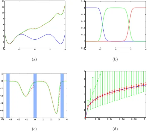
4.1. 1D triple well potential. To begin with we study diffusion in the triple well potential which is presented in Figure 4.2a. This potential has three minima at x0/1=∓3.4 andx2= 0. We chooseA= [x0−δ, x0+δ] withδ= 0.2 as the target set and the running costf =σ=const, such that the control goal is to steer the particle into C0 in minimum time. In Figure 4.2a the potential V and effective potential U are shown for= 0.5 andσ= 0.08 (solid lines), cf. equation (2.4). One can observe that the optimal control lifts the second and third well up such that the system is driven intoC0quickly.
First we validate our method with a convergence test using linear finite elements as basis functionsχi. To do so, we compute a reference solution ˆφof (3.4) using linear
finite elements on a uniform grid with spacinghr= 10−4. The resulting interpolation
φI = Piχiφ(i) is very close to the true solutionˆ φ of (3.1). We also compute a
reference solution for the value function WI = PiχiWˆ(i) with ˆW = −log ˆφ and
for the optimal controluI =−2∇WI. Then we compute coarser solutionsφI,husing
various grid spacings 1≥h≥10−3 and compute theL2 errorkφ
I,h−φIkµ, and L2
errors for WI and uI similarly. The result is shown in Figure 4.1. The L2 error of 3The Pτ do not form a semigroup since M 6= 1, thusK cannot be interpreted as i.e. the
generator of ˜Xt−. However, the entries ofKare the transition rates between the core sets as defined in transition path theory [45].
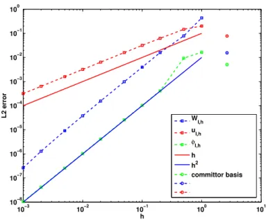
10−3 10−2 10−1 100 101 10−8 10−7 10−6 10−5 10−4 10−3 10−2 10−1 100 h L2 error W I,h u I,h φI,h h h2 committor basis Fig. 4.1: L2 error ofφ
I,h,WI,handuI,husing linear finite elements (dashed lines) and using the
committor basis (circles).
φI,h is quadratic in h, as expected from the theory. Additionally, the L2 error of
WI,his also quadratic inhwhich, given that the transformation betweenφandW is
nonlinear, is surprising. The error ofuI,his only linear inh; as expected one order of
convergence is lost due to the fact thatuI is the gradient of WI.
Next, we use a committor basis. In accordance with the strategy to minimize minimize0in Theorem 3.3, we placed core setsCi= [xi−δ, xi+δ] in each of the three
wells of the potential shown in Figure 4.2a, resulting in the set of three basis functions shown in Figure 4.2b. TheL2 errors achieved by solving (3.4) in this basis are shown as circles in Figure 4.1. We observe that the 3 committor functions achieve the same performance as linear finite elements with grid spacing h ≈0.2, which corresponds to ≈40 basis functions. Theorem 3.3 givesε0 ≤0.08, while the actual error is one order of magnitude smaller. The dashed line in Figure 4.2a gives the approximation to U calculated in the committor basis, which is in good agreement to the reference solution. In Figure 4.2c the optimal control u(solid line) and its approximation uI
(dashed line) are shown. The core sets are shown in blue. The jumps inuI at the left
boundaries of the core sets are due to the fact that the committor functions are only piecewise differentiable.
The computations so far require explicit knowledge of the basis functions χi to
compute the matricesK andF. For high-dimensional systems the committor basis is usually not explicitly known. To mimic this situation, we construct a core MSM to sample the matrices K and F. 100 trajectories of length T = 20.000 were used to build the MSM. In Figure 4.2d, the optimal cost starting from the rightmost well W(x1) and its estimate using the core MSM are shown for= 0.5 and different values of σ. Each of the 100 trajectories has seen about four transitions. For comparison, a direct sampling estimate of W(x1) using the same data is shown (green). The
direct sampling estimate suffers from a large bias and variance. In contrast, the MSM estimator for W(x1) performs well for all considered values of σ. The constant C which ensures ˆφ > 0 when σ ≤ C is approximately 0.2 in this case. This seems restrictive but still allows to capture all interesting information aboutφandW(x1).
−4 −2 0 2 4 −2 0 2 4 6 8 10 12 14 (a) −4 −2 0 2 4 −0.2 0 0.2 0.4 0.6 0.8 1 1.2 (b) −4 −3 −2 −1 0 1 2 3 4 −5 −4 −3 −2 −1 0 1 (c) 0 0.02 0.04 0.06 0.08 0.1 0 1 2 3 4 5 6 (d)
Fig. 4.2: Three well potential example for= 0.5 andσ= 0.08. (a) PotentialV(x) (blue), effective potentialU=V+ 2W(green) and approximation ofUwith committors (dashed red). (b) The three committors. (c) The optimal controlu(x) (solid line) and its approximation (dashed line). Core sets are shown in blue. (d) Optimal costW(x1) for= 0.5 as a function ofσ. Blue: Exact solution. Red: Core MSM estimate. Green: Direct sampling estimate.
4.2. Alanine dipeptide. As a second, non-trivial example we study conforma-tional transitions in Alanine dipeptide (ADP), a well-studied test system in molecular dynamics. We performed an all-atom simulation of ADP in explicit water (TIP3P) with the Amber FF99SB force field [23] using the GROMACS 4.5.5 simulation pack-age [44]. The simulations were performed in the NVT ensemble, where the temper-ature was restrained to 300 K using the V-Rescale thermostat [7]. 20 trajectories of 200ns with 100ps equilibration runs were simulated. Covalent bonds to hydrogen atoms were constrained using the LINCS algorithm11 [21] (lincs iter = 1, lincs or-der = 4), allowing for an integration timestep of 2 fs. The leap-frog integrator was used. Lennard-Jones interactions were cut off at 1 nm. Electrostatic interactions were treated by the Particle-Mesh Ewald (PME) algorithm12 [11] with a real space cut-off
of 1 nm, a grid spacing of 0.15 nm, and an interpolation order of 4. Periodic boundary conditions were applied in the x, y, and z-direction.
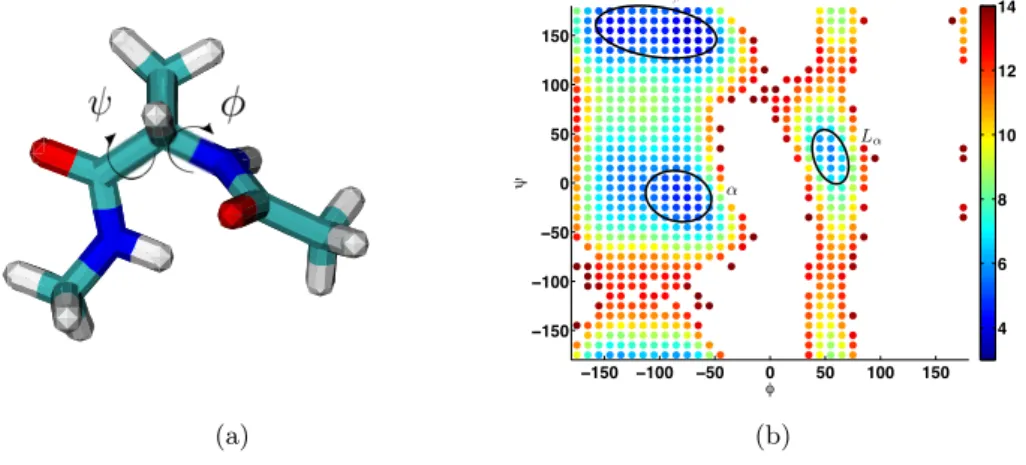
In Figure 4.3a, a cartoon of the molecule is shown. The full system including the water molecules has about 4000 degrees of freedom. However, it is well known that the conformational dynamics, which are the slowest dynamical processes in the system, can be monitored via the backbone dihedral angles φ and ψ. The dynamics along the other degrees of freedom happens on much faster timescales. For this reason, the value function will essentially be a function ofφandψ; see [19] for precise statements. We will use this to build a Markov State Model which partitions theφ−ψ-plane.
(a) −150 −100 −50 0 50 100 150 −150 −100 −50 0 50 100 150 4 6 8 10 12 14 ↵ L↵ (b)
Fig. 4.3: (a) Alanine dipeptide. (b) Free energygi=−logπi.
Validation of the MSM approximation. We construct a full partition MSM using a uniform clustering into 36×36 boxesAiof size 10◦×10◦in theφ−ψ-plane, and
we use characteristic basis functions χi(x) =1Ai for the discretization
4. Figure 4.3b shows the free energygi =−logπi=−logP[Xt∈Ai] together with the three largest
molecular conformations α, β and Lα. The missing boxes have not seen any data.
The slowest dynamical process is the switching between the left-handedLαstructure
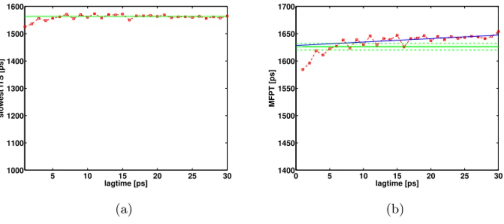
and the right-handedαandβ sheet structures. As is customary in MSM theory [35], we estimate the slowest implied timescale(ITS) as follows: For different lagtimesτ, we construct the MSM transfer operatorPτ
ij =π −1 i hχi, Tτχjiµ and compute t1(τ) =− τ logλ1(τ)
where λ1(τ) is the 2nd largest eigenvalue of Pτ. The result is shown in Figure 4.4a. We observe a plateau for 6ps ≤ τ ≤ 30ps which indicates that the time-discrete snapshots ˆXτ
n := ˆXnτ are well described by a Markov chain with transition matrix
Pτ for τ ≥ 6ps. The plateau is used to compute t1 = 1560ps±6ps. For smaller
4LetC
i⊂Ai be a core set in cellAi. The characteristic basis functions can be obtained from
the committors by expandingCi to fill out all ofAi. This basis is used to construct full partition
MSMs and produces particularly simple sampling formulas. The characteristic functions are not in
V, but the sampling results are similar to what one would obtain using committors with coresCi
which fill out most ofAi.
values of τ, ˆXτ
n is not Markovian due to recrossing effects. For this reason we also
cannot sampleK directly and have to work with the finite-time transfer operatorPτ
instead. Before proceeding to the optimal control problem, we study the effect of this time discretization on the mean first passage time (MFPT) t(x) = Ex[τα∪β] where
τα∪β is the first hitting time ofα∪β. Since theα,β andLα conformations are very
metastable,t(x) is almost constant onLαandtLα=E[t(x)|x∈Lα] can be computed
from t1 viatLα =t1/πα∪β whereπα∪β = 0.96 is the invariant measure of theαand
β conformation combined [36]. This givestLα = 1626ps±6ps.
On the other hand, let Nτ
α∪β = inf{n > 0 : ˆXnτ ∈ α∪β}. If the chain ( ˆXnτ)n
is Markovian, then the time-discrete MFPT ˆtτ(x) =E
x[τ Nατ∪β] satisfies the matrix
equation
(Pτ−I)ˆtτ =−τoutside α∪β, tˆ= 0 inα∪β. (4.1) Additionally, sinceτα∪β∈(τ(Nατ∪β−1), τ Nατ∪β], we should expect that
ˆ tτLα :=E ˆ tτ(x)|x∈Lα =tLα+cτ, c≤1. (4.2) In Figure 4.4b, ˆtτ
Lα obtained by solving (4.1) is shown as a function of τ together
with tLα. A linear interpolation using the values for 6ps ≤ τ ≤ 30ps where the
Markov assumption holds gives ˆtτ = ˆt0+ 0.8τ with ˆt0= 1628ps, which is consistent with (4.2). This shows that the time discretization introduces only small, controllable errors forτ ≥6ps. In the following, we will work withτ = 10ps. Notice that the time discretization amounts to settingK=τ−1(Pτ−I) in (3.4).
5 10 15 20 25 30 1000 1100 1200 1300 1400 1500 1600 lagtime [ps] slowest ITS [ps] (a) 0 5 10 15 20 25 30 1400 1450 1500 1550 1600 1650 1700 lagtime [ps] MFPT [ps] (b)
Fig. 4.4: (a) Slowest implied timescalet1(τ) (red) and average using the values for 6ps≤τ≤30ps (green). (b) Time-discrete MFPT ˆtτ
Lαas a function ofτ(red), linear interpolation of ˆt τ
Lα(blue) and
the reference valuetLα (green). The confidence interval oftLα is shown as dashed lines.
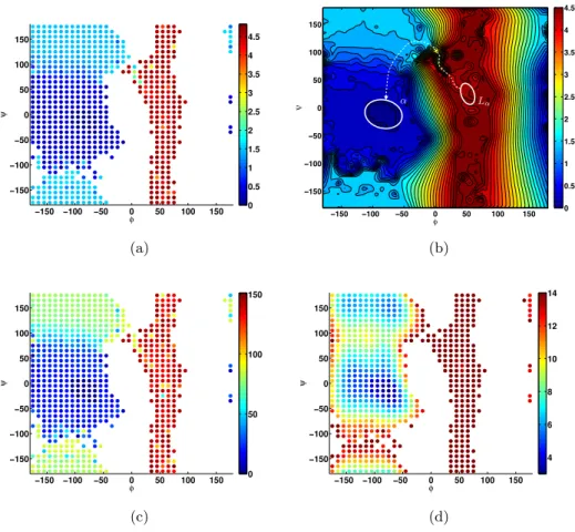
Controlled transition to the α-helical structure. Next we consider an op-timal control problem for steering the molecule into the α-structure. We choose as the target region A = α and define running costs in the (φ, ψ) variables as f(φ, ψ) = f0 +f1kψ−ψαk2 where k · k is a metric on the torus, and we choose
f0= 0.01 andf1= 0.001 representing a mild penalty for being away from the target region in theψ-direction. We discretize this control problem using the same partition
and time discretization as for the MSM construction in section 4.2 and samplePτand
F from the MSM data. The resulting value function ˆW = log ˆφis shown in Figure 4.5a. Since the basis functions χi are not differentiable and some data is missing in
ˆ
W, we have to construct an interpolationWI(φ, ψ) from the point data ˆW to obtain
as estimate for the optimal control forceu(φ, ψ) =−σ∇WI(φ, ψ). An interpolation
based on a Delauney triangulation which isC1everywhere except at the data points is shown in Figure 4.5b.
To demonstrate that adding the control force u(φ, ψ) has the effect of speeding up the transition fromLαtoα, we would have to implement it in the MD simulation
software. We leave that for future work. We can make a prediction of the anticipated effect within the MSM framework: In accordance with (2.11), we compute the tran-sition matrixPτ
v∗of the optimally controlled process byPvτ∗(i, j) =Pτ(i, j)v ∗(j)
v∗(i) with
v∗= ˆφfori6=j. The discretized MFPT vector ˆt∗ of the optimally controlled process can be computed from the Matrix equation
(Pτ
v∗−I) ˆt∗=−τ outside α, ˆt∗= 0 inα.
The result is shown in Figure 4.5c and gives a speed up compared to ˆt0 of one order of magnitude. A larger speed up could easily be achieved by increasingf. In Figure 4.5d we show the free energy of the controlled process in log scale, which according to Lemma 2.3 is given bygv∗
=−logπv∗
= logZv−2 ˆW −logπ. Observe that the
Lα and β conformations are now much less populated compared to the equilibrium
distribution in Figure 4.3b: As in the 1D example, the control mainly has the effect of lifting the wells which are not in the target region up such that they become less metastable.
5. Conclusions. We have developed a Galerkin projection method that leads to an approximation of certain optimal control problems for reversible diffusions by Markov decision problems. The approach is based on the dual formulation of the optimal control problem in terms of a linear boundary value problem that can be discretized in a straightforward way. In this article we propose a discretization that preserves reversibility and the generator form of the linear equations, i.e., the dis-cretization of the infinitesimal generator of the original diffusion process can be inter-preted as the infinitesimal generator of a reversible Markov jump process (MJP). The discretized linear boundary value problem admits again a dual formulation in terms of a Markov decision problem. A sparse approximation that uses the basis of committor functions of metastable sets of the dynamics was discussed in detail: The discretiza-tion using committor funcdiscretiza-tions does not require that the metastable sets partidiscretiza-tion the state space, hence the method can be applied to high-dimensional problems as they appear, e.g., in molecular dynamics. The committor functions in this case need not be known explicitly, as it is possible to sample the generator matrices and the discrete cost functions by a Monte-Carlo method, similarly to what is done in the Markov state modelling approach to protein folding. We could prove anL2 error estimate for the Galerkin scheme, moreover the discretization was shown to preserve basic struc-tural elements of the continuous problem, such as duality, reversibility or properties of the invariant measure. Our numerical results showed very good performance of the incomplete partition discretization on a simple toy example and a high-dimensional molecular dynamics problem, even with only a few basis functions, which is in line with the theoretical error bounds presented in this paper.
While we addressed the discretization error in this paper in great detail, we did not address the sampling error. In particular, for large systems our construction requires
−150 −100 −50 0 50 100 150 −150 −100 −50 0 50 100 150 φ ψ 0 0.5 1 1.5 2 2.5 3 3.5 4 4.5 (a) −150 −100 −50 0 50 100 150 −150 −100 −50 0 50 100 150 0 0.5 1 1.5 2 2.5 3 3.5 4 4.5 ↵ L↵ (b) −150 −100 −50 0 50 100 150 −150 −100 −50 0 50 100 150 φ ψ 0 50 100 150 (c) −150 −100 −50 0 50 100 150 −150 −100 −50 0 50 100 150 φ ψ 4 6 8 10 12 14 (d)
Fig. 4.5: (a) Optimal control ˆW for steering into the α-structure. (b) Interpolation WI(φ, ψ)
obtained from ˆW via a Delauney triangulation, and a steepest descent path fromLα to α. (c)
MFPT to theαconformation for the optimally controlled process. (d) Free energygv∗=−logπv∗
of the optimally controlled process.
the coefficients of the MJP and therefore the transition rates between all metastable states as an input. This is not fully satisfactory. We believe that the optimal control framework presented here should be linked with Monte-Carlo methods for rare events, e.g., [20, 13], that exploit the same duality between optimal control and sampling to devise efficient importance sampling strategies as we did so as to reduce the sampling error. We leave the analysis of the sampling error to future work.
Acknowledgements. The authors thank Marco Sarich and Christof Sch¨utte for helpful discussions and Antonia Mey and Francesca Vitalini for providing the Alanine dipeptide data. The research was funded by the DFG Research Centre Matheon.
Appendix A. Proof of Theorem 3.1.
Here we give the proof of Theorem 3.1 from Section 3.1. For ease of notation, let k · k=k · kµ.
Proof. Letφ be the solution to (3.2), and write φ=Qφ+φ⊥ =φ||+φ⊥ with φ⊥∈D⊥. The first step is to show thatkφ−φ||k= infψ∈Dkφ−ψk, i.e. the infimum
in the definition of ε0 is attained at φ||. But this is clear since for any ψ ∈ D, by orthogonality we have
kφ−ψ||2=kφ
||−ψ+φ⊥k2=kφ||−ψk2+kφ⊥k2 which attains its minimum of ε2
0 =kφ⊥k2 for ψ =φ||. By (3.2), φ|| solves the equation
B(φ, ψ) =B(φ||, ψ) +B(φ⊥, ψ) = 0 ∀ψ∈D,
and if we writeφ|| =Pni=1φˆ∗iχi+ 1χn+1 with n unknown coefficients ˆφ∗i (note
that a general element ofDis of this form), this takes the matrix form
ˆ
Bφˆ∗−c=F,
where in components we have ˆBij =B(χi, χj),ci =−B(φ⊥, χi) =−hφ⊥, Bχiiµ
and Fi = −hχi, Bχn+1iµ. On the other hand, the Galerkin solution ˆφ = Piφˆiχi
satisfies ˆBφˆ=F by 3.3, hence we obtain
ˆ
B( ˆφ∗−φ) =ˆ c. (A.1)
Now we can write
ε2=kφ||+φ⊥−φˆk2=kφ||−φˆk2+kφ⊥k2 = * X i ( ˆφ∗i −φˆi)χi, X j ( ˆφ∗j −φˆj)χj + µ +ε20 = ( ˆφ∗−φ)ˆ TMˆ( ˆφ∗−φ) +ˆ ε2 0
where ˆMij =hχi, χjiµ. The scalar product h·,·iµ onD0 ⊂V induces a natural scalar product onRn by the isomorphism ˆφ7→P
iφiχˆi: * X i ˆ φiχi, X j ˆ φ0jχj + µ = ˆφTMˆφˆ0 =:hφ,ˆ φˆ0iM
The errorε2 is exactly ε2
0 plus the distance between Galerkin solution and best
approximation measured in this scalar product. There is also a natural bilinear form inherited fromB onRn: B X i ˆ φiχi, X j ˆ φ0jχj = ˆφTBˆφˆ0=hφ,ˆ Mˆ−1Bˆφˆ0iM
The Matrix ˆM−1Bˆ is symmetric sinceB(·,·) is symmetric. Moreover, sinceB(·,·) is elliptic,
hφ,ˆ Mˆ−1BˆφˆiM =A X i ˆ φiχi, X j ˆ φjχj ≥α2 * X i ˆ φiχi, X j ˆ φjχj + µ =α2hφ,ˆ φˆiM (A.2) In particular, ˆM−1Bˆ is positive, hence it has a positive and symmetric square root ˆS2= ˆM−1B. Now, for any ˆˆ φ∈Rn it holds by virtue of (A.2),
hφ,ˆ φˆiM ≤ 1 α2 hφ,ˆ Mˆ−1BˆφˆiM = 1 α2 hSˆφ,ˆ SˆφˆiM ≤ 1 α2 2 hSˆφ,ˆ Mˆ−1BˆSˆφˆiM = 1 α2 2 hMˆ−1Bˆφ,ˆ Mˆ−1BˆφˆiM. (A.3)
Now we apply the inequality (A.3) to ˆφ∗−φˆand use (A.1):
ε2≤ε20+
1 α2
2
hMˆ−1c,Mˆ−1ciM. (A.4)
Now for some final simplifications, note that the orthogonal projectionQontoD0 can be written as Qψ= n X i,j=1 ˆ Mij−1hχj, ψiµχi.
Using this we can write
hMˆ−1c,Mˆ−1ciM = X ij ciMˆij−1cj = X ij hχi, Bφ⊥iµMij−1hχj, Bφ⊥iµ = * X ij Mij−1hχj, Bφ⊥iµχi, Bφ⊥ + µ =hQBφ⊥, Bφ⊥iµ =hQBφ⊥, QBφ⊥iµ
To arrive at the final result, notice that
hQBφ⊥, QBφ⊥iµ≤ sup φ0 ⊥∈D⊥ hQBφ0 ⊥, QBφ0⊥iµ hφ0 ⊥, φ0⊥iµ ! · hφ⊥, φ⊥iµ = sup φ0 ⊥∈D⊥ hQBQ⊥φ0⊥, QBQ⊥φ0⊥iµ hφ0 ⊥, φ0⊥iµ ! · hφ⊥, φ⊥iµ ≤ sup φ0∈V hQBQ⊥φ0, QBQ⊥φ0i µ hφ0, φ0i µ ! · hφ⊥, φ⊥iµ =kQBQ⊥k2hφ⊥, φ⊥iµ
Plugging these inequalities into (A.4) and dividing byε2
0 completes the proof.
Appendix B. Best-approximation error bound.
In this appendix, we prove lemma 3.3:
ε0=kQ⊥φkµ≤ kP⊥φkµ+µ(T)1/2κkfk∞+ 2kP⊥φk∞.
Recall that κ = supx∈TEx[τS\T] and P is the orthogonal projection onto the
subspaceVc={v∈L2(S, µ), v=conston everyCi} ⊂L2(S, µ). Note thatP⊥φ= 0
onC. The errorskP⊥φkandkP⊥φk∞measure how constant the solutionφis on the core sets. We writek · k=k · kµ throughout the proof for convenience.
Proof. The proof closely follows the proof of theorem (12) in [34]. The first step of the proof is to realize that the committor subspaceD where Qprojects onto can be written as D = {v ∈ L2(S, µ), v = const on every C
i, Lv = 0 on C}. To
see this, note that the values v takes on the Ci can be used as boundary values for
the Dirichlet problem Lv = 0 on T. A linear combination of committor functions is obviously a solution to this problem. But the solution to the Dirichlet problem must be unique, otherwise one can construct a contradiction to the uniqueness of the invariant distribution, see [34].
By definition we have kQ⊥φk ≤ kφ−Iφk for every interpolation Iφ∈ D of φ. With the definition ofP from above, we will take q=Iφsuch that
Lq= 0 onT, q=P φonS \T. (B.1)
NowD⊂V, thereforeq∈Vc andP q=q. Therefore (B.1) is equivalent to
P LP q= 0 onT, q=P φonS \T. (B.2) Now definee:=P φ−q. Then we have
P LP e=P LP(P φ−q) =P LP φ−P LP q=P Lφ−P LP⊥φ−P LP q and by (B.2) and sinceLφ=f φonS \A⊃T, we have
P LP e=P f φ−P LP⊥φonT, e= 0 onS \T. (B.3) Therefore, e ∈ EΘ = {v ∈ L2(S, µ), v = 0 on S \T} and with Θ being the orthogonal projection ontoEΘ,ehas to fulfil
ΘP LPΘe= ΘP f φ−ΘP LP⊥φ. Since ΘP=PΘ = Θ, this can be written as
Re:= ΘLΘe= Θf φ−ΘLP⊥φ.
The operatorR= ΘLΘ is invertible onEΘ: If this wasn’t the case, there would be a nontrivial solutionv to
Lv = 0 onT, v= 0 onS \T.
But the solution to this boundary value problem is again unique, and hence there is only the trivial solution. This gives
e=R−1Θf φ−R−1ΘLP⊥φ, (B.4)
andkR−1k= 1
|λ0| where λ0 is the principal eigenvalue of R. Due to an estimate by Varadhan we have
1
|λ0| ≤xsup∈T
Ex[τS\T] =:κ,
see e.g. [5]. To complete the derivation we need to focus on the second term in (B.4). SinceR−1 is an operator onE
Θ, we can write it asR−1ΘLP⊥φ=: Θg, where the function Θg solves
ΘLΘg=RΘg= ΘLP⊥φ⇔ΘL[Θg−P⊥φ] = 0
by the definition of R and Θg. Thereforew := Θg−P⊥φsolves the boundary value problem
Lw= 0 onT, w=−P⊥φonS \T (B.5)
which implies that kwk∞ ≤ kP⊥φk∞, this follows from Dynkin’s formula or Lemma 3 in [34]. Finally,
kΘgk ≤µ(T)1/2kΘgk
∞≤µ(T)1/2(kP⊥φk∞+kwk∞)≤2µ(T)1/2kP⊥φk∞ holds by the triangle inequality and the above considerations. Now focus on the first term in (B.4). Note that by the maximum principle,φachieves its maximum of 1 on the boundary ofS \A⊃T, therefore maxx∈T|φ(x)| ≤1. Then we have
kΘf φk ≤µ(T)1/2kfk∞max
x∈T |φ(x)| ≤µ(T)
1/2kfk ∞. Now putting everything together, we arrive at
kek ≤ kR−1kkΘf φk+kR−1ΘLP⊥φk ≤κkΘf φk+kΘgk
≤µ(T)1/2κkfk∞+ 2kP⊥φk∞
. Finally, note that by the triangle inequality
kQ⊥φk ≤ kφ−qk ≤ kφ−P φk+kP φ−qk=kP⊥φk+kek which completes the proof.
REFERENCES
[1] T. Belytschko, Y. Krongauz, D. Organ, M. Fleming, and P. Krysl, Meshless methods: An overview and recent developments, Comput. Methods Appl. M.139(1996), 3 – 47. [2] A. Berman and R.J. Plemmons,Nonnegative matrices in the mathematical sciences, Academic
Press, 1979.
[3] O. Bokanowski, J. Garcke, M. Griebel, and I. Klompmaker, An adaptive sparse grid semi-lagrangian scheme for first order Hamilton–Jacobi–Bellman equations, J. Sci. Comput.55
(2013), 575–605.
[4] M. Boulbrachene and M. Haiour, The finite element approximation of Hamilton–Jacobi– Bellman equations, Comput. Math. Appl.41(2001), 993 – 1007.
[5] A. Bovier,Methods of contemporary statistical mechanics, Metastability, Springer, 2009. [6] D. Braess,Finite elements: Theory, fast solvers, and applications in solid mechanics,
Cam-bridge University Press, 2007.
[7] G. Bussi, D. Donadio, and M. Parrinello,Canonical sampling through velocity rescaling, J. Chem. Phys.126(2007), 014101.
[8] E. Carlini, M. Falcone, and R. Ferretti,An efficient algorithm for Hamilton–Jacobi equations in high dimension, Comput. Visual. Sci.7(2004), 15–29.
[9] T. Cecil, J. Qian, and S. Osher, Numerical methods for high dimensional Hamilton–Jacobi equations using radial basis functions, J. Comput. Phys.196(2004), 327 – 347.
[10] P. Dai Pra, L. Meneghini, and W. Runggaldier, Connections between stochastic control and dynamic games, Math. Control Signals Systems9(1996), 303–326.
[11] T. Darden, D. York, and L. Pedersen,Particle mesh Ewald: AnN·log(N)method for Ewald sums in large systems, J. Chem. Phys.98(1993), 10089–10092.
[12] N. Djurdjevac, M. Sarich, and Ch. Sch¨utte,Estimating the eigenvalue error of Markov state models, Multiscale Model. Simul.10 (1)(2012), 61–81.
[13] P. Dupuis, K. Spiliopoulos, and H. Wang,Importance sampling for multiscale diffusions, Mul-tiscale Model. Simul.10(2012), 1–27.
[14] A.K. Faradjian and R. Elber,Computing time scales from reaction coordinates by milestoning, J. Chem. Phys.120(2004), 10880–10889.
[15] W.H. Fleming,Exit probabilities and optimal stochastic control, Appl. Math. Optim.4(1977), 329–346.
[16] W.H. Fleming and H.M. Soner,Controlled Markov processes and viscosity solutions, Springer, 2006.
[17] I.I. Gikhman and A.V. Skorokhod,The theory of stochastic processes II, Springer-Verlag, New York, 1975.
[18] C. Hartmann, R. Banisch, M. Sarich, T. Badowski, and Ch. Sch¨utte,Characterization of rare events in molecular dynamics, Entropy16(2014), 350–376.
[19] C. Hartmann, J.C. Latorre, G.A. Pavliotis, and W. Zhang,Optimal control of multiscale sys-tems using reduced-order models, J. Comput. Dynamics1(2014), 279–306.
[20] C. Hartmann and C. Sch¨utte,Efficient rare event simulation by optimal nonequilibrium forcing, J. Stat. Mech. Theor. Exp.11(2012), 4.
[21] B. Hess, H. Bekker, H.J.C. Berendsen, and J. Fraaije, Lincs: a linear constraint solver for molecular simulations, J. Comp. Chem.18(1997), 1463–1472.
[22] Ronald H.W. Hoppe, Multi-grid methods for Hamilton–Jacobi–Bellman equations, Numer. Math.49(1986), 239–254.
[23] V. Hornak, R. Abel, . Okur, B. Strockbine, A. Roitberg, and C. Simmerling, Comparison of multiple amber force fields and development of improved protein backbone parameters, Proteins65(2006), 712–725.
[24] C.-S. Huang, S. Wang, C.S. Chen, and Z.-C. Li,A radial basis collocation method for Hamilton– Jacobi–Bellman equations, Automatica42(2006), 2201 – 2207.
[25] H.A. Kramers,Brownian motion in a field of force and the diffusion model of chemical reac-tions, Physica7(1940), 284 – 304.
[26] Harold J. Kushner,A survey of some applications of probability and stochastic control theory to finite difference methods for degenerate elliptic and parabolic equations, SIAM Review
18(1976), 545–577.
[27] Harold J. Kushner,Numerical methods for stochastic control problems in finance, Mathematics of Derivative Securities, Cambridge University Press, 1997, pp. 504–527.
[28] H.J. Kushner and P.G. Dupuis,Numerical methods for stochastic control problems in contin-uous time, Springer Verlag, 1992.
[29] J.C. Mattingly, A.M. Stuart, and D.J. Higham,Ergodicity for SDEs and approximations: lo-cally Lipschitz vector fields and degenerate noise, Stochastic Process. Appl. 101(2002),
185–232.
[30] J. Menaldi,Some estimates for finite difference approximations, SIAM J. Control Optim.27
(1989), 579–607.
[31] B.K. Øksendal,Stochastic differential equations: An introduction with applications, Springer, 2003.
[32] M. Peletier, G. Savar´e, and M. Veneroni, Chemical reactions as Γ-limit of diffusion, SIAM Review54(2012), 327–352.
[33] H. Rabitz, R. de Vivie-Riedle, M. Motzkus, and K. Kompa,Whither the future of controlling quantum phenomena?, Science288(2000), 824–828.
[34] M. Sarich,Projected transfer operators, Ph.D. thesis, FU Berlin, 2011.
[35] M. Sarich, F. Noe, and Ch. Sch¨utte,On the approximation quality of Markov state models, Multiscale Model. Simul.8(2010), 1154–1177.
[36] Ch. Sch¨utte, F. Noe, J. Lu, M. Sarich, and E. Vanden-Eijnden,Markov state models based on milestoning, J. Chem. Phys.134(2011), 204105.
[37] Ch. Sch¨utte, S. Winkelmann, and C. Hartmann,Optimal control of molecular dynamics using Markov state models, Math. Program. (Series B)134(2012), 259–282.
[38] S. Sheu,Stochastic control and exit probabilities of jump processes, J. Control Optim.23(1985), 306–328.
[39] Q.S. Song,Convergence of Markov chain approximation on generalized HJB equation and its applications, Automatica44(2008), 761 – 766.
[40] Q.S. Song, G. Yin, and Z. Zhang,Numerical methods for controlled regime-switching diffusions and regime-switching jump diffusions, Automatica42(2006), 1147 – 1157.
[41] H. Stapelfeldt,Laser aligned molecules: Applications in physics and chemistry, Physica Scripta
2004(2004), 132–136.
[42] A. Steinbrecher,Optimal control of robot guided laser material treatment, Progress in Industrial Mathematics at ECMI 2008 (A.D. Fitt, J. Norbury, H. Ockendon, and E. Wilson, eds.), Springer Berlin Heidelberg, 2010, pp. 505–511.
[43] M. Sun, Domain decomposition algorithms for solving Hamilton-Jacobi-Bellman equations, Numer. Func. Anal. Optim.14(1993), 145–166.
[44] D. Van Der Spoel, E. Lindahl, B. Hess, G. Groenhof, A.E. Mark, and H.J. C. Berendsen,
Gromacs: Fast, flexible, and free, J. Comp. Chem.26(2005), 1701–1718. [45] E. Vanden-Eijnden,Transition path theory, Lect. Notes Phys.703(2006), 439–478.
[46] S. Wang, L.S. Jennings, and K.L. Teo,Numerical solution of Hamilton–Jacobi–Bellman equa-tions by an upwind finite volume method, J. Global Optim.27(2003), 177–192.
[47] H. Wendland, Meshless galerkin methods using radial basis functions, Math. Comput. 68
(1999), 1521–1531.
[48] M. Zhong and E. Todorov,Moving least-squares approximations for linearly-solvable stochastic optimal control problems, J. Control Theory Appl.9(2011), 451–463.