Mobile Botnet Detection: A Deep Learning Approach
Using Convolutional Neural Networks
Suleiman Y. Yerima
1and Mohammed K. Alzaylaee
2 1Cyber Technology InstituteFaculty of Computing, Engineering and Media De Montfort University, Leicester, United Kingdom
2Al-Qunfudah College of Computing Umm Al-Qura University, Saudi Arabia
Abstract— Android, being the most widespread mobile
oper-ating systems is increasingly becoming a target for malware. Ma-licious apps designed to turn mobile devices into bots that may form part of a larger botnet have become quite common, thus posing a serious threat. This calls for more effective methods to detect botnets on the Android platform. Hence, in this paper, we present a deep learning approach for Android botnet detection based on Convolutional Neural Networks (CNN). Our proposed botnet detection system is implemented as a CNN-based model that is trained on 342 static app features to distinguish between
botnet apps and normal apps. The trained botnet detection model was evaluated on a set of 6,802 real applications containing 1,929 botnets from the publicly available ISCX botnet dataset. The results show that our CNN-based approach had the highest over-all prediction accuracy compared to other popular machine learning classifiers. Furthermore, the performance results ob-served from our model were better than those reported in previ-ous studies on machine learning based Android botnet detection.
Keywords—Botnet detection; Deep learning; Convolutional Neural Networks; Machine learning; Android Botnets
I. INTRODUCTION
Android is now the most widespread mobile operating system worldwide. Over the years the volume of malware targeting Android has continued to grow [1]. This is because it is easier and more profitable for malware authors to target an operating system that is open-source, more prevalent, and does not re-strict the installation of apps from any possible source. As a matter of fact, numerous families of malware apps that are capable of infecting Android devices and turning them into malicious bots have been discovered in the wild. These An-droid bots may become part of a larger botnet that can be used to perform various types of attacks such as Distributed Denial of Service (DDoS) attacks, generation and distribution of Spam, Phishing attacks, click fraud, stealing login credentials or credit card details, etc.
A botnet consists of a number of Internet-connected devices under the control of a malicious user or group of users known as botmaster(s). It also consists of a Command and Control (C&C) infrastructure that enables the bots to receive com-mands, get updates and send status information to the mali-cious actors. Since smartphones and other mobile devices are
typically used to connect to online services and are rarely switched off, they provide a rich source of candidates for op-erating botnets. Thus, the term ‘mobile botnet’ refers to a group of compromised smartphones and other mobile devices that are remotely controlled by botmasters using C&C chan-nels [2], [3].
Nowadays, malicious botnet apps have become a serious threat. Additionally, their increasing use of sophisticated eva-sive techniques calls for more effective detection approaches. Hence, in this paper we present a deep learning approach that leverages Convolutional Neural Networks (CNN) for Android botnet detection. The CNN model employs 342 static features to classify new or previously unseen apps as either ‘botnet’ or ‘normal’. The features are extracted through automated re-verse engineering of the apps, and are used to create feature vectors that feed directly into the CNN model without further pre-processing or feature selection.
We present the design of our CNN-based model for Android botnet detection and evaluate the model on a dataset of real Android apps consisting of 1,929 botnets samples and 4,873 clean samples. Also, we compare the performance of our CNN model to other popular machine learning classifiers including Naïve Bayes, Bayes Net, Decision Tree, Support Vector Ma-chine (SVM), Random Forest, Random Tree, Simple Logistic and Artificial Neural Network (ANN) on the same dataset. The results show that the CNN-based model achieved a botnet detection performance of 98.9% with an F1-score of 0.981, thus outperforming all the other machine learning classifiers. Furthermore, our CNN model shows better performance re-sults compared to other existing studies focusing on Android botnet detection. Some of these studies utilized the same ISCX botnet apps employed in this paper.
The rest of the paper is organized as follows: Section II dis-cusses related works in Android botnet detection; Section III presents the overall system and gives some background on CNN, including a discussion of 1D CNN which is adopted in this study; Section IV presents methodology and the experi-ments performed; Results of experiexperi-ments are given in Section V and finally Section VI presents the conclusions of the study and possible future work.
II. RELATED WORK
In the study conducted by Kadir et al. [4], the objective was to address the gap in understanding mobile botnets and their communication characteristics. Thus, they provided an in-depth analysis of the Command and Control (C&C) and built-in URLs of Android botnets. By combbuilt-inbuilt-ing both static and dynamic analyses with visualization, relationships between the analysed botnet families were uncovered, offering insight into each malicious infrastructure. It is in this study that a dataset of 1929 samples of 14 Android botnet families were compiled and released to the research community. This dataset is known as the ISCX Android botnet dataset and is available from [5]. This paper and several previous works on Android botnets have utilized the full dataset or a subset of it to evaluate pro-posed Android botnet detection techniques.
Anwar et al. [6] proposed a static approach towards mobile botnet detection where they utilized MD5 hashes, permissions, broadcast receivers, and background services as features. These features were extracted from Android apps to build a machine learning classifier for detecting mobile botnet attacks. They conducted their experiments on 1400 apps from the UNB ISCX botnet dataset together with 1400 benign apps. Their best result was 95.1% classification accuracy with a recall value of 0.827 and a precision value of 0.97.
Paper [7] used machine learning to detect Android botnets based on permissions and their protection levels. The authors initially used 138 features and then added novel features known as protection levels to increase the number of features to 145. Their approach was evaluated on four machine learn-ing algorithms: Random Forest, MLP, Decision Trees and Naïve Bayes. They performed their study on 3270 app in-stances (1635 benign and 1635 botnets). The botnet apps used were also obtained from the ISCX botnet dataset. The best results came from Random Forest with 97.3% accuracy, 0.987 recall, and 0.958 precision.
In [8] a method was proposed to detect Android botnets based on Convolutional Neural Networks using permissions as fea-tures. Applications are represented as images that are con-structed based on the co-occurrence of permissions used with-in the applications. The proposed CNN is a bwith-inary classifier that is trained using the images. The authors evaluated their proposed method on 5450 Android applications consisting of 1800 botnet applications from the ISCX dataset. Their results show an accuracy of 97.2% with a recall of 0.96, precision of 0.955 and f-measure of 0.957, which is a promising result con-sidering that only permissions were used in the study.
Paper [9] proposed an Android Botnet Identification System (ABIS) for checking Android applications in order to detect botnets. ABIS utilized both static and dynamic features from API calls, permissions and network traffic. The system is evaluated by using several machine learning algorithms with Random Forest obtaining a precision of 0.972 and a recall of 0.969. In [10], a method is proposed for Android botnet
detec-tion based on feature selecdetec-tion and classificadetec-tion algorithms. The paper used ‘permissions requested’ as features and ‘In-formation gain’ to select the most significant permissions. Afterwards, Naïve Bayes, Random Forest and Decision Trees were used to classify the Android apps. Results show Random Forest achieving the highest detection accuracy of 94.6% with the lowest false positive rate of 0.099.
Karim et al [11] proposed DeDroid, a static analysis approach to investigate botnet-specific properties that can be used to detect mobile botnets. They first identified ‘critical features’ by observing the coding behaviour of a few known malware binaries having C&C features. They then compared these ‘crit-ical features’ with features of malicious applications from the Drebin dataset [12]. Through this comparison, 35% of the ma-licious apps in the dataset qualified as botnets. However, clos-er examination revealed that 90% wclos-ere confirmed as botnets. Bernardeschia et al. [13] proposed a method to identify bot-nets in Android environment through model checking. Model checking is an automated technique for verifying finite state systems. This is accomplished by checking whether a structure representing a system satisfies a temporal logic formula de-scribing their expected behaviour. In [14], Jadhav et al. pro-pose a cloud-based Android botnet detection system which exploits dynamic analysis by using a virtual environment with cluster analysis. The toolchain for the dynamic analysis pro-cess within the botnet detection system is composed of strace, netflow, logcat, sysdump, and tcpdump. However, the authors did not provide any experimental results to evaluate the effec-tiveness of their proposed solution. Moreover, botnets may easily employ different techniques to evade the virtual envi-ronment, and code coverage could limit the system’s effec-tiveness [15], [24].
Paper [16] proposed an approach to detect mobile botnets us-ing network features such as TCP/UDP packet size, frame duration, and source/destination IP address. The authors used a set of ML box algorithms and five machine learning classifi-ers to classify network traffic. The five supervised machine learning approaches include Naïve Bayes, Decision Tree, K-nearest neighbour, Neural Network, and Support Vector Ma-chine. In [17], a method to detect Android botnets based on source code mining and source code metric was proposed. There are also a number of works that have proposed signature based methods for Android botnet detection. These include [18-20]. However, these solutions are likely to suffer from the drawbacks of signature based systems which includes the ina-bility to effectively detect previously unseen botnets.
Unlike most existing studies, our paper proposes a deep learn-ing based Android botnet detection system, uslearn-ing Convolu-tional Neural Networks. Also, unlike previous studies that utilize only the app permissions, our system is based on 342 features that represent Permissions, API calls, Commands, Extra Files, and Intents. Furthermore, different from the study in [9] which utilized only permissions, we do not convert
fea-ture vectors into images prior to model training. Instead our feature vectors are used directly to train 1D CNN models. This makes our approach computationally less demanding.
III. BACKGROUND A. The CNN-based classification system
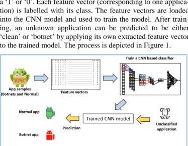
The classification system is built by extracting static features from the corpus of botnet and clean samples. To achieve this, we used our bespoke tool built in Python for automated re-verse engineering of APKs. With the help of the tool, we ex-tracted 342 features consisting of five different types (see Ta-ble 2) from all the training apps. The five feature types in-clude: API calls extracted from the executable; Permissions and Intents from the manifest file; Commands and Extra Files from the APK. These features are represented as vectors of binary numbers with each feature in the vector represented by a ‘1’ or ‘0’. Each feature vector (corresponding to one applica-tion) is labelled with its class. The feature vectors are loaded into the CNN model and used to train the model. After train-ing, an unknown application can be predicted to be either ‘clean’ or ‘botnet’ by applying its own extracted feature vector to the trained model. The process is depicted in Figure 1.
Figure 1: Training and prediction with the CNN-based botnet detection system.
B. Convolutional Neural Networks (CNN)
A CNN is a deep learning technique that belongs to the family of Artificial Neural Networks. It works well for identifying simple patterns in the data which will then be used to form more complex patterns in higher layers. Two types of layers are typically used for building CNNs; convolutional layers and pooling layers. The role of the convolutional layer is to detect local conjunctions of features from the previous layer, while the role of the pooling layer is to merge semantically similar features into one [21].
Generally, the convolutional layer extracts the optimal fea-tures while the pooling layer reduces the dimensions of those features that it receives from the convolutional layer (or an-other preceding pooling layer). At the tail end of the model, fully connected (dense) layer(s) are typically used for classifi-cation. Depending on the characteristics of the dataset, the performance of the CNN may be influenced by the number of layers, number of filters (kernels) or the size of the filters. Generally, more and more abstract features are extracted in the
deeper layers of the CNN, hence, the number of layers re-quired depends on the complexity and non-linearity of the data being analysed. Furthermore, the number of filters in each stage determines the number of features extracted. Computa-tional complexity increases with more layers and higher num-bers of filters. Also, with more complex architectures, there is the possibility of training an overfitted model which results in poor prediction accuracy on the testing set(s). To reduce over-fitting, techniques such as ‘dropout’ [22] and ‘batch regulari-zation’ are implemented during training of our models. C. One Dimensional Convolutional Neural Networks Although CNN is more commonly applied in a multi-dimensional fashion and has thus found success in image and video analysis-based problems, they can also be applied to one-dimensional data. Datasets that possess a one-dimensional structure can be processed using a one-dimensional convolu-tional neural network (1D CNN). The key difference between a 1D and a 2D or 3D CNN is the dimensionality of the input data and how the filter (feature detector) slides across the data. For 1D CNN, the filters only slide across the input data in one direction. A 1D CNN is quite effective when you expect to derive interesting features from shorter (fixed-length) seg-ments of the overall feature set, and where the location of the feature within the segment is not of high relevance.
The use of 1D CNN can be commonly found in NLP applica-tions. Similarly, 1D CNN is applicable to datasets containing vectorised data being used to characterize the items to be pre-dicted (e.g. an Android application). The 1D CNN could be used to extract potentially more discriminative feature repre-sentations that describe any existing patterns or relationships within segments of the vectors characterizing each entity in the dataset. These new features are then fed into a classifier (e.g. a fully connected neural network layer) which will in turn use the derived features in making a final classification deci-sion. Hence, in this scenario, the convolutional layers can be considered as a feature extractor that eliminates the need for feature ranking and selection. The CNN model developed in this paper is applied to vectorised data characterizing the An-droid applications, in order to derive a trained model that can detect new Android botnet apps with very high accuracy. D. Key elements of our proposed CNN architecture
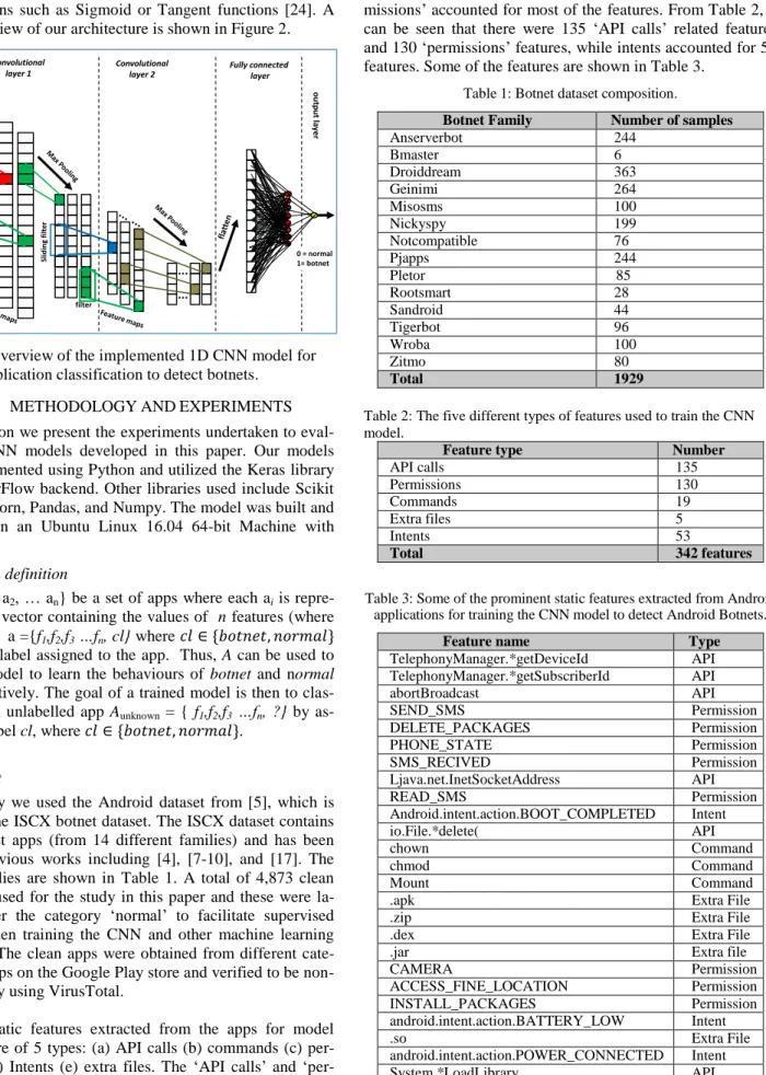
Our proposed CNN architecture is a 1D CNN consisting of two convolutional layers and two max pooling layers. These are followed by a fully connected layer of N units, which is in turn connected to a final classification layer containing one neuron with a sigmoid activation function.
The sigmoid activation function is given by: 𝑆 = 1
1+ 𝑒−𝑥
The final classification layer generates an outcome corre-sponding to the two classes i.e. ‘botnet’ or ‘normal’. The con-volutional layers utilize the ReLU (Rectified Linear Units) activation function given by: 𝑓(𝑥) = max(0, 𝑥). ReLU helps to mitigate vanishing and exploding gradient issues [23]. It has been found to be more efficient in terms of time and cost for training huge data in comparison to classical non-linear activa-App samples
(Botnets and Normal)
f1 f2 f3 f4 f5 f6 ………f342 Class 0 1 0 1 1 0 ……… 1 N 1 1 0 0 1 0 ……… 1 N 1 0 0 1 0 1 ……… 0 B 0 1 0 0 1 0 ……… 1 N 0 1 0 1 1 1 ……… 0 B 1 1 0 0 1 0 ……… 0 N 0 1 0 1 0 1 ……… 1 N 1 0 0 0 0 0 ……… 1 B 0 0 0 1 0 0 ……… 0 N 1 1 0 0 0 0 ……… 1 N 0 0 0 1 1 1 ……… 0 B 0 1 0 0 1 0 ……… 1 B 0 1 0 1 1 1 ……… 1 N . . . . . . . . . . . . . . . . Trained CNN model
Prediction Unclassified application Feature vectors
Train a CNN based classifier
Botnet app Normal app
tion functions such as Sigmoid or Tangent functions [24]. A simplified view of our architecture is shown in Figure 2.
Figure 2: Overview of the implemented 1D CNN model for Android application classification to detect botnets.
IV. METHODOLOGY AND EXPERIMENTS
In this section we present the experiments undertaken to eval-uate the CNN models developed in this paper. Our models were implemented using Python and utilized the Keras library with TensorFlow backend. Other libraries used include Scikit Learn, Seaborn, Pandas, and Numpy. The model was built and evaluated on an Ubuntu Linux 16.04 64-bit Machine with 4GB RAM.
A. Problem definition
Let A ={a1, a2, … an} be a set of apps where each ai is repre-sented by a vector containing the values of n features (where n=342). Let a ={f1,f2,f3 …fn, cl} where 𝑐𝑙 ∈ {𝑏𝑜𝑡𝑛𝑒𝑡, 𝑛𝑜𝑟𝑚𝑎𝑙} is the class label assigned to the app. Thus, A can be used to train the model to learn the behaviours of botnet and normal apps respectively. The goal of a trained model is then to clas-sify a given unlabelled app Aunknown = { f1,f2,f3 …fn, ?} by as-signing a label cl, where 𝑐𝑙 ∈ {𝑏𝑜𝑡𝑛𝑒𝑡, 𝑛𝑜𝑟𝑚𝑎𝑙}.
B. Dataset
In this study we used the Android dataset from [5], which is known as the ISCX botnet dataset. The ISCX dataset contains 1,929 botnet apps (from 14 different families) and has been used in previous works including [4], [7-10], and [17]. The botnet families are shown in Table 1. A total of 4,873 clean apps were used for the study in this paper and these were la-belled under the category ‘normal’ to facilitate supervised learning when training the CNN and other machine learning classifiers. The clean apps were obtained from different cate-gories of apps on the Google Play store and verified to be non-malicious by using VirusTotal.
The 342 static features extracted from the apps for model training were of 5 types: (a) API calls (b) commands (c) per-missions (d) Intents (e) extra files. The ‘API calls’ and
‘per-missions’ accounted for most of the features. From Table 2, it can be seen that there were 135 ‘API calls’ related features and 130 ‘permissions’ features, while intents accounted for 53 features. Some of the features are shown in Table 3.
Table 1: Botnet dataset composition.
Botnet Family Number of samples
Anserverbot 244 Bmaster 6 Droiddream 363 Geinimi 264 Misosms 100 Nickyspy 199 Notcompatible 76 Pjapps 244 Pletor 85 Rootsmart 28 Sandroid 44 Tigerbot 96 Wroba 100 Zitmo 80 Total 1929
Table 2: The five different types of features used to train the CNN model.
Feature type Number
API calls 135 Permissions 130 Commands 19 Extra files 5 Intents 53 Total 342 features
Table 3: Some of the prominent static features extracted from Android applications for training the CNN model to detect Android Botnets.
Feature name Type
TelephonyManager.*getDeviceId API TelephonyManager.*getSubscriberId API abortBroadcast API SEND_SMS Permission DELETE_PACKAGES Permission PHONE_STATE Permission SMS_RECIVED Permission Ljava.net.InetSocketAddress API READ_SMS Permission Android.intent.action.BOOT_COMPLETED Intent io.File.*delete( API chown Command chmod Command Mount Command
.apk Extra File
.zip Extra File
.dex Extra File
.jar Extra file
CAMERA Permission
ACCESS_FINE_LOCATION Permission
INSTALL_PACKAGES Permission
android.intent.action.BATTERY_LOW Intent
.so Extra File
android.intent.action.POWER_CONNECTED Intent
System.*LoadLibrary API
Input layer Convolutional
layer 1 Fully connectedlayer
o u tp u t la yer Convolutional layer 2 Slidi ng fil ter Slidi ng fil ter filter Slidi ng fil ter filter 0 = normal 1= botnet L = 342
C. Experiments to evaluate the proposed CNN based model In order to investigate the performance of our proposed model, we performed different sets of experiments. Table 4 shows the configuration of the CNN model. The 1D CNN model consists of two pairs of convolutional and maxpooling layers as shown in Figure 2. The output of the second max pooling layer is flattened and passed on to a fully connected layer with 8 units. This is in turn connected to a sigmoid activated output layer containing one unit.
The first set of experiments was aimed at evaluating the im-pact of number of filters on the model’s performance. The second set of experiments was performed to evaluate the effect of varying the length of the filters. In the third, we investigate the impact of the maxpooling size on performance.
Table 4: Summary of model configurations.
Model design summary -1D CNN Input layer: Dimension = 342 (feature vector size) 1D Convolutional layer: 4, 8, 16, 32, 64 filters, size = 4, 8, 16, 32, 64 (with number of filters =32)
MaxPooling layer: Size =2, 4, 8, 16 (with number of filters =32) 1D Convolutional layer: 4, 8, 16, 32, 64 filters,
size = 4, 8, 16, 32, 64 (with number of filters =32)
MaxPooling layer: Size =2, 4, 8, 16 (with number of filters =32) Fully Connected (Dense) layer: 8 units, activation=ReLU Output layer: Fully Connected layer; 1 unit, activa-tion=sigmoid
In order to measure model performance, we used the follow-ing metrics: Accuracy, precision, recall and F1-score. The metrics are defined as follows (taking botnet class as positive):
Accuracy: Defined as the ratio between correctly pre-dicted outcomes and the sum of all predictions. It is given by: TP+TN
TP+TN+FP+FN
Precision: All true positives divided by all positive predictions. i.e. Was the model right when it predict-ed positive? Given by: TP
TP+FP
Recall: True positives divided by all actual positives. That is, how many positives did the model identify out of all possible positives? Given by: TP
TP+FN
F1-score: This is the weighted average of precision and recall, given by: 2 x Recall x Precision
Recall+Precision
Where TP is true positives; FP is false positives; FN is false negatives, while TN is true negatives (all w.r.t. the botnet class). All the results of the experiments are from 10-fold cross validation where the dataset is divided into 10 equal parts with 10% of the dataset held out for testing, while the models are trained from the remaining 90%. This is repeated until all of the 10 parts have been used for testing. The average
of all 10 results is then taken to produce the final result. Also, during the training of the CNN models (for each fold), 10% of the training set was used for validation.
V. RESULTS AND DISCUSSIONS
A. Varying the numbers of filters.
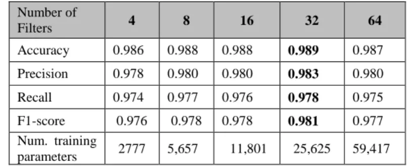
In this section, we examine the results from experimenting with different numbers of filters. In our model, we kept the number of filters in both convolutional layers the same. Table 5 shows the results from running the 1D CNN model with different numbers of filters. From the table, it is evident that the number of filters had an effect on the performance of the model. When increased from 4 to 8, there is an improvement in performance. The performance does not improve until we reach 32 filters. It then drops again when we increase this to 64. Based on these results we select 32 filters as the optimal configuration parameter for the model’s number of filters. Notice the increase in the number of training parameters as the number of filters is increased, and for 32 filters, the training of 25,625 parameters is required. With 32 filters we obtain a classification accuracy of 98.9% compared to 98.6% that is obtained with 4 filters. Nevertheless, the results obtain with 4 filters were still acceptable.
1) Training epochs, loss and accuracy graphs.
Figures 3 and 4 shows the typical outputs obtained with the validation and training sets during the training epochs. From Fig. 3, it can be seen that the validation loss is generally fluc-tuating from one training epoch to another after an initial drop. During each epoch, a model is trained and the validation loss and accuracy are recorded. Our goal is to obtain the model with the least validation loss because we assume this will be the ‘best’ model that fits the training data. Thus, at every epoch, the validation loss is compared to previous ones and if the current one is lower, the corresponding model is saved as the best model. We implemented a ‘stopping criterion’ which will stop the training once no improvement in performance is observed within 100 epochs. For example in Figure 3, the best model was obtained with the least validation loss of 0.00531 at epoch 45. For the next 100 epochs validation loss did not im-prove, hence the training was stopped. Figure 4 shows the corresponding accuracy behaviour observed from epoch to epoch.
Table 5: Number of filters vs. model performance. Length of filters used= 4 for first layer and =4 for second layer; dense layer = 8 units; validation split=10%.
Number of Filters 4 8 16 32 64 Accuracy 0.986 0.988 0.988 0.989 0.987 Precision 0.978 0.980 0.980 0.983 0.980 Recall 0.974 0.977 0.976 0.978 0.975 F1-score 0.976 0.978 0.978 0.981 0.977 Num. training parameters 2777 5,657 11,801 25,625 59,417
Figure 3: Training and validation losses at different epochs up to 145. A stopping criterion of 100 is used to obtain the model with the least validation loss.
Figure 4: Training and validation accuracies at different epochs up to 145. These plots correspond to the training and validation losses depicted in Figure 3.
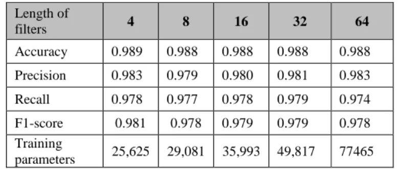
B. Varying the length of the filters.
In this section we examine the effect of the length of filters on the performance of the model while the number of filters is fixed at 32 in each convolutional layer. The length is varied from 4, 8, 16, 32, to 64 respectively (as shown in Table 6). The number of units in the dense layer was fixed at 8. The results indicate that the length of the filters does not appear to have much of an impact on the overall classification accuracy and F1-score performance, when increased. However, the least filter length of 4 achieves the highest accuracy and F1-score. Note that as we increase the length of the filters, the number of parameters to be trained increases (from 25,652 for length=4 to 77,465 for length=64).
The lack of improvement with the length of filters may be attributed to larger number of parameters leading to overfitting the model to the training data thereby reducing its generaliza-tion capability. This in turn leads to degraded performance when tested on new data. Basically, what these results show is that when the training parameters increase beyond a certain limit, the model becomes too complex for the data and this leads to overfitting. This becomes evident in lack of improve-ment or degradation in performance when tested on previously unseen data.
Table 6: Length of filters vs. model performance. Number of filters used= 32 in both first and second convolutional layers; dense layer = 8 units; validation split=10%.
Length of filters 4 8 16 32 64 Accuracy 0.989 0.988 0.988 0.988 0.988 Precision 0.983 0.979 0.980 0.981 0.983 Recall 0.978 0.977 0.978 0.979 0.974 F1-score 0.981 0.978 0.979 0.979 0.978 Training parameters 25,625 29,081 35,993 49,817 77465
C. Varying the Maxpooling parameter
The results of the third set of experiments are discussed here. The goal is to investigate the effect of changing the maxpool-ing parameter. This corresponds to a subsamplmaxpool-ing ratio of 2, 4, 6, and 8 respectively as shown in Table 7. A value of 2 means the next layer will be half the dimension of the previous one, etc. Note that the maxpooling layer can be considered a fea-ture reduction layer that also helps to alleviate overfitting since it progressively reduces the number of parameters that need to be trained. The other parameters were fixed as fol-lows: Number of filters in both convolutional layers = 32; Length of convolutional filters = 4; number of units in dense layer=8.
It can be seen from Table 7 that as we increase the maxpool-ing parameter, the total number of trainmaxpool-ing parameters is re-duced. At the same time, we witness a progressive decline in overall performance. Therefore, for our CNN model designed to classify applications into ‘botnet’ and ‘normal’, the optimal subsampling ratio for both layers is 2.
Table 7: Maxpooling parameter vs. model performance. Length of filters used=4 for both convolutional layers; number of filters =32 for both layers; dense layer = 8 units; validation split=10%. Maxpooling parame-ter/Subsampling ratio 2 4 6 8 Accuracy 0.989 0.987 0.983 0.978 Precision 0.983 0.982 0.974 0.971 Recall 0.978 0.973 0.967 0.948 F1-score 0.981 0.978 0.970 0.959 Training Parameters 25,625 9497 6,425 5,401
D. CNN performance vs. other machine learning classifiers: 10 fold cross validation results.
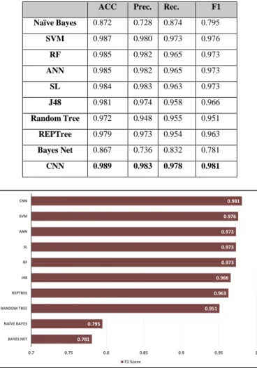
In Table 8, the performance of the CNN model developed in this paper is compared to other machine learning classifiers: Naïve Bayes, SVM, Random Forest, Artificial Neural Net-work, J48, Random Tree, REPtree, and Bayes Net. Figure 5 shows the F1-scores of the classifiers, where CNN has the
highest F1-score (0.981), followed by SVM (0.976), SL (0.973), ANN (0.973) and Random Forest (0.973). Bayes Net had the least F1-score of 0.781. Table 8 shows that the recall of CNN is 0.978 which indicates that it has the best botnet detection performance than the other classifiers. Note that the ANN was a back propagation neural network built with a sin-gle hidden layer consisting 32 units (neurons). The sigmoid activation function was used within the neurons. This ANN represented the application of a neural network without deep learning. The ANN showed no significant improvement in the results when the number of units in the hidden layer was in-creased beyond 32.
Table 8: Comparison of our CNN results with results from other ML classifiers.
ACC Prec. Rec. F1
Naïve Bayes 0.872 0.728 0.874 0.795 SVM 0.987 0.980 0.973 0.976 RF 0.985 0.982 0.965 0.973 ANN 0.985 0.982 0.965 0.973 SL 0.984 0.983 0.963 0.973 J48 0.981 0.974 0.958 0.966 Random Tree 0.972 0.948 0.955 0.951 REPTree 0.979 0.973 0.954 0.963 Bayes Net 0.867 0.736 0.832 0.781 CNN 0.989 0.983 0.978 0.981
Figure 5: F1-score of CNN vs other ML classifiers. E. Comparison with other works on Android botnet detection. In Table 9, we present a comparison of our results with those reported in other papers that focus on Android botnet detection. Note that all the papers mentioned in the table have used the ISCX botnet dataset for their work. In our study we utilized the entire 1929 samples within the dataset. In the second column of the table, the numbers of botnet samples and benign samples used in the papers are shown, while the other columns contain the performance results. Not all of the performance metrics we
have used are reported in every paper. Nevertheless, it is clear that our CNN model obtained better overall accuracy, F1 and recall than the other works.
Table 9: performance comparisons with other works. Note that all of the papers used botnets samples from the ISCX dataset.
Paper reference Botnets /Benign ACC (%) Rec. Prec. F1 Hojjatinia et al. [8] 1800/3650 97.2 0.96 0.955 0.957 Tansettanakorn et al. [9] 1926/150 - 0.969 0.972 - Anwar et. al [6] 1400/1400 95.1 0.827 0.97 - Abdullah et al. [10] 1505/850 - 0.946 0.931 - Alqatawna & Faris [7] 1635/1635 97.3 0.957 0.987 -
This paper 1929/4873 98.9 0.978 0.983 0.981
VI. CONCLUSIONS AND FUTURE WORK
In this paper, we proposed a deep learning model based on 1D CNN for the detection of Android botnets. We evaluated the model through extensive experiments with 1,929 botnet apps and 4,387 clean apps. The model outperforms several popular machine learning classifiers evaluated on the same dataset. The results (Accuracy: 98.9%; Precision: 0.983; Recall: 0.978; F1-score: 0.981) indicate that our proposed CNN based model can be used to detect new, previously unseen Android botnets more accurately than the other models. For future work, we will aim to improve the model training process by automating the search and selection of the key influencing parameters (i.e. number of filters, filter length, and number of fully connected (dense) layers) that jointly result in the optimal performing CNN model.
REFERENCES
[1] S. Y. Yerima and S. Khan “Longitudinal Perfomance Anlaysis of Machine Learning based Android Malware Detectors” 2019 International Conference on Cyber Security and Protection of Digital Services (Cyber Security), IEEE
[2] H. Pieterse and M. S. Olivier, "Android botnets on the rise: Trends and characteristics," 2012 Information Security for South Africa, Johannesburg, Gauteng, 2012, pp. 1-5.
[3] Letteri, I., Del Rosso, M., Caianiello, P., Cassioli, D., 2018. Performance of botnet detection by neural networks in software-defined networks, in: CEUR WORKSHOP PROCEEDINGS, CEUR-WS.
[4] Kadir, A.F.A., Stakhanova, N., Ghorbani, A.A., 2015. Android botnets: What urls are telling us, in: International Conference on Network and System Security, Springer. pp. 78–91.
[5] ISCX Android botnet dataset. Available from https://www.unb.ca/cic/datasets/android-botnet.html. [Accessed 03/03/2020]
[6] S. Anwar, J. M. Zain, Z. Inayat, R. U. Haq, A. Karim, and A. N. Jabir, "A static approach towards mobile botnet detection," in 2016 3rd International Conference on Electronic Design (ICED), 2016: IEEE, pp. 563-567.
[7] J. f. Alqatawna and H. Faris, "Toward a Detection Framework for Android Botnet," in 2017 International Conference on New Trends in Computing Sciences (ICTCS), 2017: IEEE, pp. 197-202.
[8] S Hojjatinia, S Hamzenejadi, H Mohseni, “Android Botnet Detection using Convolutional Neural Networks” 28th Iranian Conferenc on
Electircal Engineering (ICEE2020).
[9] C. Tansettanakorn, S. Thongprasit, S. Thamkongka, and V. Visoottiviseth, "ABIS: a prototype of android botnet identification 0.781 0.795 0.951 0.963 0.966 0.973 0.973 0.973 0.976 0.981 0.7 0.75 0.8 0.85 0.9 0.95 1 BAYES NET NAÏVE BAYES RANDOM TREE REPTREE J48 RF SL ANN SVM CNN F1 Score F1 Score
system," in 2016 Fifth ICT International Student Project Conference (ICT-ISPC), 2016: IEEE, pp. 1-5.
[10] Z. Abdullah, M. M. Saudi, and N. B. Anuar, "ABC: android botnet classification using feature selection and classification algorithms," Advanced Science Letters, vol. 23, no. 5, pp. 4717-4720, 2017. [11] Karim, Ahmad & Salleh, Rosli & Shah, Syed. (2015). DeDroid: A
Mobile Botnet Detection Approach Based on Static Analysis. 10.1109/UIC-ATC-ScalCom-CBDCom-IoP.2015.240.
[12] The Drebin Dataset. Available at: https://www.sec.cs.tu-bs.de/~danarp/drebin/index.html [accessed 05/03/2020]
[13] Cinzia Bernardeschia, Francesco Mercaldo, Vittoria Nardonec, Antonella Santoned, Exploiting Model Checking for Mobile Botnet Detection. 23rd International Conference on Knowledge-Based and Intelligent Information & Engineering Systems. Procedia Computer Science 159 (2019) 963–972.
[14] Jadhav, S., Dutia, S., Calangutkar, K., Oh, T., Kim, Y.H., Kim, J.N., 2015. Cloud-based android botnet malware detection system, in: Advanced Communication Technology (ICACT), 2015 17th International Conference on, IEEE. pp. 347–352.
[15] S. Y. Yerima, M. K. Alzaylaee, and S. Sezer. “Machine learning-based dynamic analysis of Android apps with improved code coverage” EURASIP Journal on Information Security, 4 (2019). https://doi.org/10.1186/s13635-019-0087-1
[16] Meng, X. and Spanoudakis, G. (2016). MBotCS: A mobile botnet detection system based on machine learning. Lecture Notes in Computer Science, 9572, pp. 274-291. doi: 10.1007/978-3-319-31811-0_17 [17] B. Alothman and P. Rattadilok ‘Android botnet detection: An integrated
source code mining aproach’ 12th International Conference for Internet Technology and Secured Transactions (ICITST),11-14 Dec.,Cambridge, UK, 2017, IEEE, pp 111-115.
[18] A. J. Alzahrani and A. A. Ghorbani, "Real-time signature-based detection approach for sms botnet," in 2015 13th Annual Conference on Privacy, Security and Trust (PST), 2015: IEEE, pp. 157-164.
[19] D. A. Girei, M. A. Shah, and M. B. Shahid, "An enhanced botnet detection technique for mobile devices using log analysis," in 2016 22nd International Conference on Automation and Computing (ICAC), 2016: IEEE, pp. 450-455.
[20] M. Yusof, M. M. Saudi, and F. Ridzuan, "A New Android Botnet Classification for GPS Exploitation Based on Permission and API Calls," in International Conference on Advanced Engineering Theory and Applications, 2017: Springer, pp. 27-37.
[21] Y. LeCun, Y.Bengio, and G. Hinton, Deep learning, Nature 521 (2015), no. 7553, 436-444
[22] N. Srivastava, G. Hinton, A. Krizhevsky, I. Stuskever, and R. Salakhutdinov. “Dropout: A simple way to prevent neural networks from overfitting” The Journal of Machine Learning Research, 15(1):1929-1958, 2014.
[23] X. Glorot, A. Bordes, and Y. Bengio, ‘‘Deep sparse rectifier neural networks,’’ in Proc. 14th Int. Conf. Artif. Intell. Statist., 2011, pp. 315– 323.
[24] M. K. Alzaylaee, S. Y. Yerima, Sakir Sezer “DL-Droid: Deep learning based android malware detection using real devices” Computers & Security, Volume 89, 2020, 101663, ISSN 0167-4048, https://doi.org/10.1016/j.cose.2019.101663.