Multi-stage mixed rule learning approach for advancing performance of rule-based classification

This is an Open Access document downloaded from ORCA, Cardiff University's institutional repository: http://orca.cf.ac.uk/122359/

This is the author’s version of a work that was submitted to / accepted for publication. Citation for final published version:

Liu, Han and Chen, Shyi-Ming 2019. Multi-stage mixed rule learning approach for advancing performance of rule-based classification. Information Sciences 495 , pp. 65-77.

10.1016/j.ins.2019.05.008 file

Publishers page: http://dx.doi.org/10.1016/j.ins.2019.05.008 <http://dx.doi.org/10.1016/j.ins.2019.05.008>

Please note:

Changes made as a result of publishing processes such as copy-editing, formatting and page numbers may not be reflected in this version. For the definitive version of this publication, please refer to the published source. You are advised to consult the publisher’s version if you wish to cite

this paper.

This version is being made available in accordance with publisher policies. See

http://orca.cf.ac.uk/policies.html for usage policies. Copyright and moral rights for publications made available in ORCA are retained by the copyright holders.

1

Multi-stage mixed rule learning approach for advancing

performance of rule-based classification

Han Liu

, Shyi-Ming Chen

a_{School of Computer Science and Informatics, Cardiff University}

Cardiff, United Kingdom

b_{Department of Computer Science and Information Engineering, National}

Taiwan University of Science and Technology, Taipei, Taiwan *Corresponding Author.

E-mail addresses: [email protected] (H. Liu),

[email protected] (S.-M. Chen)

____________________________________________________________________

Abstract

Rule learning is a special type of machine learning approaches, and its key advantage is the generation of interpretable models, which provides a transparent process of showing how an input is mapped to an output. Traditional rule learning algorithms are typically based on Boolean logic for inducing rule antecedents, which are very effective for training models on data sets that involve discrete attributes only. When continuous attributes are present in a data set, traditional rule learning approaches need to employ crisp intervals. However, in reality, problems usually show shades of grey, which motivated the development of fuzzy rule learning approaches by employing fuzzy intervals for handling continuous attributes. While a data set contains a large portion of discrete attributes or even no continuous attributes, fuzzy approaches cannot be used to learn rules effectively, leading to a drop in the performance. In this paper, a multi-stage approach of mixed rule learning is proposed, which involves strategic combination of both traditional and fuzzy approaches to handle effectively various types of attributes. We compare our proposed approach with existing algorithms of rule learning. Our experimental results show that our proposed approach leads to significant advances in the performance compared with the existing algorithms.

Keywords: Fuzzy classification; Fuzzy rules; Machine learning; Rule learning.

_____________________________________________________________________ 1. Introduction

Rule learning is one of the popular approaches of machine learning, especially given its advantage on interpretation of how a rule based model is used to map an input into an output. In the algorithmic setting, rule learning can be achieved through two main strategies, namely, divide and conquer (DAC) and separate and conquer (SAC). The DAC strategy aims at generating a set of rules automatically represented in the

2

form of a decision tree [25], i.e., each individual rule can be extracted from a branch of the tree (traversing from the root to a leaf node). Therefore, the DAC strategy is also known as the Top-Down Induction of Decision Trees (TDIDT) [29]. In contrast, the SAC strategy aims at generating a set of rules in the ‘if-then’ form directly from training data in a sequential manner [28], i.e., one rule is generated first and the instances covered by this rule are deleted from the training set before initiating the generation of the next rule on the basis of the remaining instances. Therefore, the SAC strategy is also known as the covering approach [30]. In order to distinguish these two strategies, we use the two terms ‘decision tree learning’ and ‘rule learning’ for referring to the DAC strategy and the SAC strategy, respectively, in the rest of this paper.

In practice, both the decision tree learning and rule learning approaches can be used for classification and regression tasks in the setting of supervised learning, depending on the actual type of data outputs. In particular, when the output is discrete (categorical), the supervised learning task needs to be defined as training of classification models (classifiers). Therefore, the trained decision trees or rules can be referred to as classification trees or classification rules in this context. When the output is continuous (numerical), the supervised learning task needs to be defined as training of regression models. Therefore, the trained decision trees or rules can be referred to as regression trees or regression rules in this context.

In this paper, we focus on classification tasks and investigate effective ways of advancing the performance of rule-based classification. Traditional approaches are typically based on Boolean logic, which indicates that the generated rules involve one or more hard conditions [30], i.e., a rule cannot be used to classify an instance unless some attribute values of the instance are satisfactory (meeting all the conditions). In this setting, the outcome of rule-based classification would be deterministic so the trained rules are usually called deterministic rules [29].

In real word applications, traditional approaches that are used to train deterministic rules can generally result in a high risk of overfitting, due to two main reasons. Firstly, real data usually remain a high level of uncertainty [31]. For example, the data quality is unknown indicating the possible case of noise [24]. Also, real data are likely to be incomplete and it is very uncertain how well the data can be representative of a full population (data distribution) in a specific domain [23]. From the above points of view, deterministic rules trained on real data would be less generalizable, leading to the case that the hard conditions involved in the rules can leave new instances uncovered by any of the rules or make new instances incorrectly covered by one or some of the rules. In other words, due to the low generalizability of the deterministic rules, new instances are likely to be incorrectly classified or unclassified, while the binary truth value (indicating that the joint conditions involved in a rule are fully met or not) is shifted

3

sharply from 0 to 1 or in the opposite way. On the other hand, the majority of real world problems cannot be simply formulated as black and white, i.e., these problems show some shades of grey [22, 45]. For example, a condition may be partially met to a certain degree although it is not fully met. On the basis of the above argumentation, fuzzy logic has been employed more popularly for reducing the risk of overfitting and advancing the performance of rule-based classification.

Although fuzzy rule learning approaches can be used to deal more effectively with continuous attributes in comparison with traditional rule learning approaches, while a data set contains only discrete attributes or a small portion of continuous attributes, traditional approaches would be more suitable, since fuzzy approaches cannot handle discrete attributes leading to a drop in the classification performance. In this context, it would be very necessary to propose a mixed rule learning approach that is capable of handling more effectively various types of attributes. On the other hand, existing approaches of rule learning typically involve only a single stage of learning. In order to increase the depth of learning, it has become more necessary to let a learning approach involve multiple stages. In this paper, we thus propose a mixed rule learning approach, which involves a multi-stage fuzzy rule learning part for handling continuous attributes in more depth and a traditional rule learning part for handling both discrete attributes and continuous attributes in diverse ways. In this way, we can achieve to take advantages of fuzzy approaches for handling continuous attributes without loss of the effectiveness of dealing with discrete attributes.

The rest of this paper is organized as follows. Section 2 provides a review of rule learning and some existing algorithms are analyzed in details for identifying their key limitations. In Section 3, we present some preliminaries on fuzzy logic and rule-based classification and illustrate our proposed multi-stage approach of mixed rule learning. In Section 4, we provide details on the setting of our experiments and discuss the experimental results. In Section 5, we draw the conclusions by stressing the contributions of our work and suggesting some further directions.

2. Related Work

As mentioned in Section 1, the rule-based models trained through the DAC and SAC strategies are automatically represented in two different forms. In particular, the former strategy leads to the automatic representation of decision trees, whereas the latter directly results in the representation of ‘if-then’ rules. The main reason is due to the essential difference between learning of decision trees and learning of ‘if-then’ rules in terms of algorithmic design [25]. In other words, decision tree learning is achieved essentially through recursive selection of attributes for the nodes of the decision tree

4

being trained, whereas rule learning is achieved through iterative selection of attribute-value pairs to form the antecedents of the rule being learned [28].

In the context of decision tree learning, the most classic algorithms include ID3 [38], C4.5 [40] and CART [5]. In particular, the ID3 algorithm is designed to employ entropy or information gain as the heuristics for attribute selection, i.e., for each node of the decision tree being trained, the attribute that obtains the minimum entropy or the maximum information gain is selected to show how a training set is split into subsets. The ID3 algorithm has demonstrated the capability of training decision trees that show very high accuracy of classification especially on the chess end game data set [37]. However, the ID3 algorithm can only handle discrete attributes, i.e., when continuous attributes are present in a data set, it is necessary to employ a method of discretization to change the numeric values of each attribute into multiple intervals [8]. In order to achieve direct handling of continuous attributes as part of the decision tree generation process, the C4.5 algorithm was proposed in [40] as a successor of the ID3 algorithm. In addition, the C4.5 algorithm was also enhanced to deal directly with missing values, which usually occur from real data.

On the other hand, the CART algorithm was developed in [5] for generating binary decision trees, which is essentially different from the ID3 and C4.5 algorithms in terms of dealing with multi-valued discrete attributes. In particular, when a discrete attribute

Ai involves more than two categorical values, if ID3 or C4.5 is adopted for training a

decision tree, the selection of the attribute Ai for a non-leaf node would result in m

branches corresponding to the m values of the selected attribute Ai, towards growing

the tree. In contrast, if the CART algorithm is adopted, the non-leaf node resulting from the selection of the attribute Ai would only lead to two branches – one showing the

positive case (e.g., ‘age= young’) and the other showing the negative case (e.g., ‘age≠ young’). For the above example, if the attribute ‘age’ contains three values, namely, ‘young’, ‘old’ and ‘middle-aged’, then the selected value ‘young’ would be judged as the most effective one to discriminate between different classes. More details on the difference between ID3/C4.5 and CART have been explained in [25].

Since decision tree learning algorithms generally have the risk of producing models that overfit training data, more researchers have been motivated to develop pruning algorithms to simplify decision trees for improving the generalizability. For example, the reduced error pruning (REP) algorithm [10] has been successfully applied to the C4.5 algorithm for simplifying decision trees [39]. Also, the cost complexity pruning (CCP) algorithm [6] has been effectively used for simplifying decision trees that are trained using the CART algorithm [11]. Some other popular pruning algorithms include the pessimistic error pruning (PEP) algorithm [35] and the minimum error pruning (MEP) algorithm [36]. On the other hand, ensemble learning approaches have

5

been used to boost the effectiveness of decision tree learning. For example, the Bagging [5], Random Subspace [15] and Boosting [12] approaches have been used jointly for creating decision tree ensembles. In addition, several other ways have been taken for advancing the performance of decision tree learning algorithms, namely, incorporating cost functions into the heuristics for attribute selection [20] and employing fuzzy logic [44] for fuzzification of continuous attributes to train fuzzy decision trees [2, 18, 19]. As pointed out in [13], decision tree learning algorithms usually result in the production of complex trees, even if pruning algorithms are used for simplification. On the other hand, it has been pointed out by Cendrowska in [7] that decision tree learning algorithms can lead to the replicated subtree problem, which not only increases the risk of overfitting but also results in high computational complexity. In order to address the above issue, it has been the motivation for some researchers to develop algorithms for learning rules by following the SAC strategy. In particular, the Prism algorithm was developed in [7] as a representative example of rule learning algorithms. Another popular algorithm of rule learning is called Ripper [9].

The nature of the Prism algorithm is to select in turn each of the predefined K classes as the target class and then learn a set of rules from the training set for the target class, i.e., there are totally K sets of rules learned in parallel from the same training set and each rule is learned by discriminating the target class from the other classes. This target class based strategy of learning usually results in a large number of rules that could form a complex rule-based classifier [28]. In order to achieve the complexity reduction, some pruning algorithms have been adopted to simplify rules that are generated using the Prism algorithm, e.g., Jmid-pruning [32]. Also, the PrismCTC algorithm has recently been developed in [28] as a variant of the Prism algorithm through modifying the target class selection strategy, for both improving the classification performance and reducing the complexity of the trained rule-based classifiers. In addition, the Information Entropy based rule generation (IEBRG) [26] and Gini-Index Based Rule Generation (GIBRG) [25] algorithms have been developed by shifting the learning strategy to a non-target class based one, for overcoming the limitations of the Prism algorithm, i.e., the learning of each rule is achieved through discrimination between different classes without the need of selecting a target class.

The nature of the Ripper algorithm is to select iteratively an attribute-value pair as a rule antecedent, based on the FOIL information gain [9]. Since the algorithm involves a pruning action taken as soon as a rule is completely generated and a global optimization stage is involved after the whole rule set has been generated, the algorithm is more robust to noisy data and thus less likely to result in overfitting, in comparison to the Prism algorithm. However, the Ripper algorithm is still based on Boolean logic leading to the production of deterministic rules. When a data set contains a large number

6

of continuous attributes with high variability on the attribute domains, it would still be difficult to avoid overfitting, due to the case that the binary truth value that shows whether an instance is covered by a rule can be shifted sharply from 0 to 1 (or in the opposite way), even if the values of some attributes are just changed slightly. In order to make the Ripper algorithm more robust, the Fuzzy Unordered Rule Induction Algorithm (FURIA) has been developed in [16] for fuzzifying the antecedents of each rule generated using the Ripper algorithm, which has led to an improvement of the performance of rule-based classification.

FURIA is a fuzzy rule learning algorithm that does not need to consider all continuous attributes for generating rule antecedents, which is different from those earlier fuzzy rule learning algorithms that typically employ all continuous attributes for generating rule antecedents, e.g., the mixed fuzzy rule formation algorithm [4]. However, in reality, it is very likely that a data set contains not only continuous attributes but also discrete attributes. In this case, fuzzy rule learning approaches that only consider continuous attributes for generating rule antecedents would not be capable to perform well on learning rules from the above-mentioned type of data sets. Moreover, existing approaches of fuzzy rule learning typically involve only a single learning stage based on the crisp labels originally assigned to training instances. As mentioned in Section 1, real data may show some shades of grey, which indicates the necessity to include the intensity score (membership degree) for each class as a new continuous attribute (numeric label) of an instance for fuzzy rule learning. In Section 3, we will introduce how to achieve numeric labelling of instances for in-depth learning of fuzzy rules alongside diversified learning of traditional rules, through adopting our proposed multi-stage approach of mixed rule learning.

3. Multi-stage approach of mixed rule learning

In this section, some preliminaries are provided to introduce the theories of fuzzy logic and fuzzy rule-based systems. Furthermore, our proposed multi-stage approach of mixedrule learning is illustrated in details and some theoretical justifications are also given to show how the proposed approach can be more effective to lead to advances in the performance of rule-based classification.

3.1 Preliminaries

Fuzzy logic is based on the fuzzy set theory [44], which employs a fuzzy membership degree ∈ [0, 1]instead of a binary membership degree ∈ {0, 1} for making a judgement. In the context of machine learning, fuzzy classification is achieved by measuring the degree to which an instance xi belongs to a class ct, i.e., the membership

degree _�� � , where the class ct is considered as a fuzzy set S and the instance xj is

7

of an element e to a fuzzy set S, a membership function ս needs to be defined for the fuzzy set S as shown in Fig. 1 as an example of a popularly used trapezoidal membership function, where the horizontal axis indicates the numeric value v of a continuous attribute x (i.e., an element of the fuzzy set S) and the vertical axis indicates the membership degree of the value of attribute x to the fuzzy set S (i.e., ). In machine learning, the purpose of defining a membership function is to fuzzify a continuous attribute, i.e., it is to map the numeric value of a continuous attribute of an instance to the membership degree of this numeric value to a fuzzy set defined for the continuous attribute.

Fig. 1. Trapezoidal membership function [22]

The definition of a membership function can be achieved in practice by using expert knowledge or through inductive reasoning on real data. As shown in Fig. 1, the essence of defining a membership function is to determine the four parameters a, b, c and d for the trapezoidal shape, where b and c are defined, respectively, as the lower bound and the upper bound of the core region [b, c] for an element to obtain a full membership to the fuzzy set, and a and d are defined, respectively, as the lower bound and the upper bound of the support region (a, b) (c, d) for an element to gain a non-zero membership degree to the fuzzy set. When the upper bound and the lower bound of the core region are equal, i.e., b = c, then the defined membership function would become triangular and the core region would be represented by a single point at which the membership degree of an element for the fuzzy set is equal to 1. There is another extreme case that the shape of the membership function becomes rectangle and thus there is no support region available for an element of the fuzzy set to obtain a membership degree between 0 and 1, i.e., ∈ { , }, while a = b and c = d.

Fuzzy classification is typically undertaken by constructing a fuzzy-rule based system, which can be represented in the following form:

8

Rule 2: if A1 is T12 and A2 is T22 and … and Ad is Td2 then class = c2,

⁞

Rule m: if A1 is T1m and A2 is T2m and … and Ad is Tdm then class = cm.

In the setting of fuzzy rule learning, each antecedent (e.g., A1 is T11) of a fuzzy rule is

generated essentially through defining a fuzzy set Tik for an attribute Ai. The number of

antecedents for each rule is the same as the dimensionality of the training data if the fuzzy rule learning algorithm, e.g. the mixed fuzzy rule formation algorithm [4], needs to select all continuous attributes. In contrast, there are also some algorithms that do not need to consider all continuous attributes for generating fuzzy rules, e.g., FURIA [16]. In this case, the number of antecedents for each rule is usually less than (but possibly equal to) the dimensionality of the training data that contain only continuous attributes. The above set of fuzzy rules represents the case that each rule has a unique consequent (class), but it is possible in real world applications that some rules have the same consequent (class), i.e., the number of classes may be less than m.

In the fuzzy rule-based classification stage, there are generally three main operations, namely, fuzzification, inference and defuzzification. The fuzzification operation is to transform the numeric value of each attribute Ai of the instance xj into

the membership degree to a fuzzy set Tik defined for attribute Ai involved in rule Rr. The

inference operation is to compute the firing strength of each rule Rr using a T-norm, i.e.,

to compute the membership degree of the instance xj to the class ct shown in the

consequent of rule Rr. Based on the firing strength of each rule Rr, we can compute the

overall membership degree of the instance xj to each class c using a T-cornorm, i.e.,

this is to combine the firing strengths of the rules for each class ct to obtain the overall

membership degree of the instance xj to ct.

A T-norm is essentially to conjunct the membership degrees obtained from all the antecedents of rule Rr, which show the degrees to which the values of the attributes of

the instance xj satisfy the antecedents of rule Rr. Some commonly used T-norms include

the Min T-norm (Eq. (1)) [44], the Product T-norm (Eq. (2)) [14], Lukasiewicz’s T-norm (Eq. (3)) [34] and Yager’s T-norm (Eq. (4)) [43] are shown as follows:

⊤ ( ), ( ) , … , ( ) = min_{≤ ≤} { _�( )}, (1)

⊤ ( ), ( ) , … , ( ) = ∏= _�( ), (2)

⊤ ( ), ( ) , … , ( ) = �{ , ∑= _�( ) − } , (3)

9

In Eqs. (1)–(4), Si denotes the fuzzy set defined for the attribute Ai and vij is the value

of attribute Ai of the instance xj.

A T-cornorm is essentially to combine the membership degrees ��(� ), ��(� ) , … , �� (� ) obtained from multiple rules R1, R2, …, Rm for the same

class ct so that we can compute the overall membership degree of the instance xj to the

class ct. Some commonly used T-cornorms included the Max T-cornorm (Eq. (5)) [44],

the Product T-cornorm (Eq. (6)) [14], Lukasiewicz’s T-cornorm (Eq. (7)) [34] and Yager’s T-cornorm (Eq. (8)) [43] are shown as follows:

⟘ ��(� ), ��(� ) , … , �� (� ) = max_{≤ ≤} { ���(� )} , (5) ⟘ _��(� ), _��(� ) , … , _�� (� ) = ∑ _���_{(� )} = − ∏ = ���(� ), (6) ⟘ _��(� ), _��(� ) , … , _�� (� ) = � { , ∑ _���_{(� )} = } , (7) ⟘ ��(� ), ��(� ) , … , �� (� ) = � { , ∑ ���(� ) � = �}. (8) Each T-norm has a corresponding T-cornorm (e.g., the Min T-norm is dual to the Max T-cornorm under the order revising operation) and they make up a dual pair that is referred to as fuzzy norm. Therefore, the above four pairs of T-norms and T-cornorms shown in Eqs. (1)–(8) can be referred to as the Min/Max norm, the Product norm, Lukasiewicz’s norm and Yager’s norm. From Eqs. (4) and (8), we can see that Yager’s norm involves a power parameter ѡ. When the value of the parameter ѡ is set to 1, Yager’s norm would be identical to Lukasiewicz’s norm, which indicates that Lukasiewicz’s norm is a special case of Yager’s norm. According to the empirical investigation made in [14], a popular value set for the power parameter ѡ is 2, and we can thus refer it to as Yager’s [2.0] norm, which is the one used in this paper for experimentation (to be reported in Section 4).

After the overall membership degree of the instance xj to each class ct is obtained,

the final classification is made through the defuzzification operation by assigning the instance xj the class cmax that obtains the maximum membership degree.

3.2 The proposed multi-stage approach of mixed rule learning

The proposed multi-stage approach of mixed rule learning involves two main parts. The first part is to create a decision tree ensemble that consists of two decision trees as the base classifiers, where the first base classifier is trained on the original feature set using the C4.5 algorithm without pruning and the second base classifier is trained by

10

discretizing all continuous attributes in the original feature set by using Fayyad and Irani’s MDL method [11] and then using the preprocessed feature set to build a decision tree using C4.5 with reduced error pruning [10]. The second part is to create mn (1≤ n

≤ N) fuzzy ensembles at each of the predefined N stages of fuzzy rule learning, while

m shrink heuristics are used for conflict avoidance. In particular, each single fuzzy

rule-based classifier is trained using the mixed fuzzy rule formation algorithm [4] with a selected fuzzy norm (e.g., the Min/Max norm) as well as a selected shrink heuristic (e.g., border-based shrink), and then algebraic fusion of the fuzzy rule-based classifiers trained using the same shrink heuristic is taken using a fusion rule. In this section, we describe the whole procedure of the proposed multi-stage approach of mixed rule learning in a step-by-step manner.

The whole procedure is also illustrated in Fig. 2, which shows that a decision tree ensemble is simply created only at the first stage of training but multiple fuzzy ensembles are created at each training stage. In particular, each fuzzy ensemble consists of f fuzzy rule-based classifiers, which are trained using the f selected fuzzy norms, respectively. However, the f fuzzy rule-based classifiers in the same ensemble need to be trained using the same shrink heuristic. According to the empirical investigation in [14], both shrink heuristics and fuzzy norms can have impacts on the performance of the mixed fuzzy rule formation algorithm. Therefore, we adopt m shrink heuristics to achieve effective creation of diversity externally among m fuzzy ensembles and also adopt f fuzzy norms to create diversity internally among f fuzzy rule-based classifiers in the same ensemble.

In terms of training a single fuzzy classifier, the mixed fuzzy rule formation algorithm is designed essentially to learn fuzzy rules sequentially in an instance-by-instance manner, i.e., each instance-by-instance is checked, and then a new rule is generated or some existing rules are adjusted. In the whole procedure, there may be three possible cases, namely, ‘covered’, ‘commit’ and ‘shrink’. In particular, if an instance xj is not covered

by any existing rules, then the ‘commit’ case is reached and a new rule Rt is generated

to cover this instance xj by setting fuzzy sets involved in the rule antecedents. In order

to let the instance xj obtain the membership degree of 1 to the generated rule Rt, each

fuzzy set Si shown in an antecedent of this rule Rt is defined by initializing the lower

and upper bounds (bi and ci) of the core region of Si according to the value vij of the

attribute Ai of this instance xj and initializing the lower and upper bounds (ai and di) of

the support region to cover the entire domain of the attribute Ai. For example, if the

value vij of the attribute Ai is 2.2 and the domain of this attribute is [1.1, 5.6], then the

initialized values of a, b, c and d would be 1.1, 2.2, 2.2 and 5.6, respectively. Once a new rule Rt is generated, a so-called anchor ⃗ is set as a parameter, which remembers

11

epoch of fuzzy rule learning for further adjusting the set of generated fuzzy rules (to be discussed later in this section).

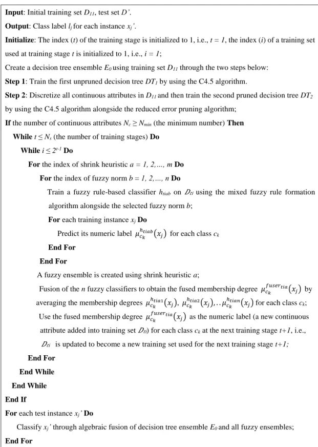
Input: Initial training set D11, test set D’.

Output: Class label lj for each instance xj’.

Initialize: The index (t) of the training stage is initialized to 1, i.e., t = 1, the index (i) of a training set used at training stage t is initialized to 1, i.e., i = 1;

Create a decision tree ensemble E0 using training set D11 through the two steps below:

Step 1: Train the first unpruned decision tree DT1 by using the C4.5 algorithm.

Step 2: Discretize all continuous attributes in D11 and then train the second pruned decision tree DT2

by using the C4.5 algorithm alongside the reduced error pruning algorithm; If the number of continuous attributes Nc˅ Nmin (the minimum number) Then

While t ˄ Ns (the number of training stages) Do

While i ˄ 2t-1 _Do

For the index of shrink heuristic a = 1, 2,…, m Do For the index of fuzzy norm b = 1, 2,…, n Do

Train a fuzzy rule-based classifier htiab on �i using the mixed fuzzy rule formation algorithm alongside the selected fuzzy norm b;

For each training instance xj Do

Predict its numeric label _�

�

ℎ�� _{(� ) for each class ck}

End For End For

A fuzzy ensemble is created using shrink heuristic a;

Fusion of the n fuzzy classifiers to obtain the fused membership degree _�� �� (� ) by averaging the membership degrees _�ℎ_��� (� ), _�ℎ_��� (� ), . . _�ℎ_��� (� ) for each class ck;

Use the fused membership degree _�� �� (� ) as the numeric label (a new continuous attribute added into training set �i) for each class ck at the next training stage t+1, i.e.,

�i is updated to become a new training set used for the next training stage t+1;

End For End While End While End If

For each test instance xj’ Do

Classify xj’ through algebraic fusion of decision tree ensemble E0 and all fuzzy ensembles;

End For

12

If an instance xj is already covered by an existing rule Rk, i.e., the instance xj has a

membership degree _�(� ) ∈ , ] to the rule Rk, then the ‘covered’ case is reached.

In this case, the core regions of some fuzzy sets shown in some antecedents of the rule

Rk need to be adjusted by letting the values of the corresponding attributes fall into the

core regions of these fuzzy sets, such that the instance xj will obtain a full membership

(i.e., _�(� ) = ) to the rule Rk. In other words, for each attribute Ai, if its value vij

does not yet fall into the core region [bik, cik] of the corresponding fuzzy set Si, then the

lower or upper bound (bik or cik) of the core region needs to be modified to ensure ≤

≤ , such that the membership degree of the value vij of the attribute Ai is equal to

1, i.e., _�( ) = . Overall, once the ‘covered’ case is reached, the rule Rk that covers

the instance xj must beadjusted to enable that the instance xj falls into the core region

([b1k, c1k] [b2k, c2k] … [bnk, cnk]) of the rule Rk.

For both the ‘covered’ and ‘commit’ cases, it is necessary to take the shrink action to avoid conflict of classification. In particular, when an instance � ∈ is covered by a rule Rt of class ≠ , then the rule Rt must be adjusted to let the instance xj obtain

no membership (i.e., _�(� ) = ) to the rule. The conflict of classification may involve two possible cases: (1) the instance xj obtains a partial membership (the

membership degree _�( ) ∈ , ) to the rule Rt; (2) the instance xj obtains a full

membership (the membership degree _�( ) = ) to the rule Rt. In the first case, the

conflict of classification can be avoided without loss of rule coverage (instances of class

cl covered by rule Rt), by adjusting the support regions of the fuzzy sets shown in some

antecedents of the rule Rt. In the second case, the conflict of classification cannot be

avoided without loss of rule coverage, which means that some instances of cl covered

by rule Rt will be lost due to the adjustments of the core regions of the fuzzy sets shown

in some antecedents of the rule Rt. Three shrink heuristics, namely, area-based shrink,

anchor-based shrink and rule-based shrink, have been proposed and investigated empirically in [14] with more details on how to achieve conflict avoidance effectively. Once all the training instances have been checked, the first epoch of fuzzy rule learning is completed and we obtain an initial set of fuzzy rules. At this point, it is necessary to adjust all the rules by turning the core region ([b1k, c1k] [b2k, c2k] …

[bnk, cnk]) of each rule Rk back to the original status ([v1j, v1j] [v2j, v2j] … [vnj, vnj])

13

maintaining the support region ([(a1k, b1k) (c1k, d1k)] [(a2k, b2k) (c2k, d2k)] … [(ank, bnk) (cnk, dnk)]) of each rule. In other words, for each fuzzy set Si shown in an antecedent

of rule rk, the core region [bik, cik] of Si needs to be reset to [vij, vij], while the support

region (aik, bik) (cik, dik) of Si remains unchanged. In this way, the core regions of the

fuzzy rules are adjusted based on the training instances covered by these rules and this process is repeated for several further epochs until no new rule is generated and/or no conflict of classification occurs. As indicated in [4], the above process of resetting and adjusting the generated rules usually needs a small number (less than 10) of epochs. In the worst case, the number of epochs would not exceed a maximum that is equivalent to the total number of training instances. In practice, the maximum number of epochs for training a set of fuzzy rules can also be predefined.

In terms of algebraic fusion of fuzzy classifiers, when different fuzzy norms are used as parameters of the mixed fuzzy rule formation algorithm, multiple fuzzy classifiers with diversity can be trained to make up a fuzzy ensemble. In this context, we can fuse multiple fuzzy classifiers by combining the membership degrees estimated by these classifiers for each class. In other words, each instance xj would be assigned

different membership degrees for each class by using different fuzzy classifiers. In order to reduce the potential estimation error of the membership degree for each class, it has been a popular practice to combine the membership degrees estimated by different classifiers through using a fusion rule [17], such as mean (Eq. (9)), max (Eq. (10)), median (Eq. (11)) and product (Eq. (12)), shown as follows:

�� (� ) = ∑ℎ= �ℎ�(� ), (9)

�� (� ) = max_≤ℎ≤ { �ℎ�(� )}, (10)

�� (� ) = med_≤ℎ≤ { �ℎ�(� )}, (11)

�� (� ) = ∏ℎ= �ℎ�(� ). (12) In Eqs. (9)–(12), ck denotes a class with the index of k and xj represents an unseen

instance that is being classified. The denotation _�ℎ_�(� ) represents the membership degree of instance xj estimated by classifier h for class ck and _�� (� ) thus denotes

the overall membership degree of instance xj obtained for each class ck through

combining the membership degrees _��(� ), _��(� ), … , _��(� ) estimated by the m classifiers. In this paper, we take the mean rule (shown in Eq. (9)) for algebraic fusion of multiple fuzzy classifiers, since it is the one most popularly used in practice [17].

14

After fusion of multiple fuzzy classifiers, the combined membership degree �� (� ) of each instance xj for each class ck is used as a numeric label (a new continuous attribute) of the instance xj for the next stage of fuzzy rule learning.

Generally speaking, at each stage (except for the first stage) of fuzzy rule learning, multiple fuzzy classifiers are trained separately on the instances that are assigned the numeric labels as new continuous attributes, which are essentially the membership degrees _� (� ), _� (� ), … , _� (� ) for the n predefined classes) obtained through taking the outputs of the algebraic fusion of the fuzzy classifiers trained at the previous stage. For example, at the first stage of fuzzy rule learning, there are four classifiers trained on the instances that are assigned the original class labels (ground truth). After fusion of the four classifiers, for each instance xj, combined membership

degrees _� (� ), _� (� ), … , _� (� ) are obtained for the n predefined classes and will be used as n numeric labels for training four new classifiers at the next stage. The same operation also applies to each test instance for getting n numeric labels used at the next stage of testing. This process is repeated until the required number of training stages is reached.

The n numeric labels of each instance xj in a newly created training set for the n

predefined classes can be obtained through two ways. In particular, the first way is achieved by using a previously obtained training set for training m fuzzy classifiers and then using each of the m trained fuzzy classifiers to predict the membership degrees �ℎ(� ), �ℎ(� ), … , �ℎ (� ) of each instance xj for the n classes c1, c2, …, cn. In this

way, for each instance xj, m membership degrees can be obtained for each class ck, so a

combined membership degree for each class ck can be obtained through fusing the m

fuzzy classifiers. Finally, the combined membership degrees

� (� ), � (� ), … , � (� ) forthe n classes c1, c2, …, cn are used as the n

numeric labels of instance xj in the newly created trained set used for the next stage of

fuzzy rule learning and ensemble creation.

The second way of obtaining the n numeric labels of each instance xj in a newly

created training set is to conduct 10-fold cross validation on the training set. In this way, each of the training instances will be treated as an unseen one in a specific one of the 10 folds and will thus obtain n membership degrees for the n classes as predicted by using one of the m fuzzy classifiers trained in the specific fold. Similar to the first way described above, the m trained fuzzy classifiers will be fused to obtain combined

15

membership degrees _� (� ), _� (� ), … , _� (� ) for the n classes c1, c2,…, cn, which will be finally used as the n numeric labels of instance xj in the new created

training set used for the next stage of fuzzy rule learning and ensemble creation. In general, the first way of numeric labelling would be more recommended than the second way, since 10-fold cross validation may result in the case that training instances may not be well representative of test instances in some of the 10 folds. In this case, it is very likely to result in incorrect estimation of the fuzzy membership degrees for the classes, which could introduce noise in the values of the newly added continuous attributes (resulting from numeric labelling of instances). In other words, it is crucial to make sure the numeric labelling of instances is highly confident to avoid noise in values of the newly added continuous attributes. In this case, the newly added continuous attributes can be used as additionally helpful features for learning fuzzy rules of better quality.

The idea of the above multi-stage fuzzy rule learning approach is naturally inspired from the theory of deep neural networks in a layer-by-layer processing manner. For our proposed approach, the depth depends on the number (N) of training stages, whereas the width depends on the number of trained fuzzy classifiers that make up a fuzzy ensemble and the number of fuzzy ensembles. From an ensemble learning perspective, it is crucial that each single classifier trained as a member of an ensemble must not be too weak in terms of its classification performance and different classifiers that make up the ensemble need to be diverse and complementary to each other, such that the fusion of these classifiers in the ensemble can lead to an effective improvement of the overall performance of classification [17]. Similarly, multiple fuzzy ensembles created using different shrink heuristics also need to be diverse and complementary to each other. From this point of view, the increase of depth would aim for improving the overall classification performance, whereas the increase of the width aims to increase the diversity between the trained classifiers to maximize the chance for the classifiers in an ensemble to be more complementary to each other. The main focus of this paper is thus on the increase of both the depth and the width in advancing the performance of rule-based classification.

Finally, all the fuzzy rule ensembles created at the N stages of training are fused in an algebraic rule with a decision tree ensemble created at the first stage of training, in order to avoid the case that fuzzy approaches cannot learn effectively from a data set that contains a very small portion of or even no continuous attributes, leading to low performance of rule-based classification. Also, when a data set contains a large portion of continuous attributes, various ways of handling continuous attributes through both fuzzy and traditional rule learning approaches would be likely to lead to the effective

16

creation of diversity among different classifiers or ensembles, which again indicates the necessity to adopt fusion of the fuzzy ensembles and the decision tree ensemble, towards advances in the performance of rule-based classification.

4.Experimental results

Some experiments are conducted in this section, by using 20 data sets retrieved from the UCI machine learning repository [21]. Some of the data sets contain both discrete and continuous attributes, whereas the other data sets contain only one type of attributes, i.e., either discrete attributes or continuous attributes. The details of the selected data sets are provided in Table 1 in terms of their characteristics.

Table 1

Data sets used for experiments.

Dataset name Number of discrete/continuous attributes Number of instances Number of classes Anneal Balance-scale Breast-cancer Breast-w Credit-a Credit-g Cylinder-bands Dermatology Diabetes Hepatitis Ionosphere Iris Kr-vs-kp Labor Lymph Sponge Tae Vote Wine Zoo 32/6 0/4 9/0 0/9 9/6 13/7 21/18 33/1 0/8 13/6 0/34 0/4 36/0 8/8 15/3 45/0 2/3 16/0 0/13 16/1 898 625 286 699 690 1000 540 366 768 155 351 150 3196 57 148 76 151 435 178 101 6 3 2 2 2 2 2 6 2 2 2 3 2 2 4 3 3 2 3 7

In the setting of the proposed multi-stage approach of mixed rule learning, the creation of the decision tree ensemble is achieved to train two decision trees as base classifiers at the first stage of training only, where the first base classifier is trained simply on the original feature set using the C4.5 algorithm without the simplification

17

of the trained decision tree through pruning and the second base classifier is trained through first discretizing all the continuous attributes in the feature set and then building the decision tree on the preprocessed feature set with simplification of the trained decision tree using the reduced error pruning algorithm [10].

The creation of fuzzy rule ensembles at each stage of training is achieved to adopt two shrink heuristics (anchor-based shrink and border-based shrink) for creating two fuzzy ensembles on each of the feature sets given at a specific stage of training. For example, at the first stage of training, there is only an original feature set so two ensembles are created on the feature set in total using the anchor-based shrink and the border-based shrink, respectively. At the second stage of training, there are two newly created training sets, since the two fuzzy ensembles created at the first stage of training can assign each instance two different membership degrees for each class, i.e., two different sets of continuous attributes (reflecting the membership degrees for the classes) are separatelyadded to the original feature set to get two new training sets (containing all attributes in the original feature set + newly added continuous attributes). In this context, there are totally four fuzzy ensembles created at the second stage of training on the two new training sets given at this stage, i.e. on each of the two new training sets, there are two fuzzy rule ensembles created using the anchor-based shrink and the border-based shrink, respectively. In our experiments, the number of training stages (N) is set to 2, due to the general small size of each data set. In terms of creation of each of the fuzzy rule ensembles, four fuzzy rule-based classifiers are trained using the four fuzzy norms, namely, the Min/Max Norm, the Product Norm, Lukasiewicz’s Norm and Yager’s Norm, while the same shrink heuristic is used for avoiding conflict of classification, i.e., the shrink heuristic used for creation of a fuzzy ensemble is either anchor-based shrink or border-based shrink.

In terms of internal fusion of the base classifiers in an ensemble and external fusion of multiple ensembles, the mean rule is used in general. However, when a data set contains a small portion of continuous attributes, it is more likely to result in the case that the performance of the decision tree ensemble could be considerably better than the performance obtained through fusion of all the fuzzy ensembles. In the above case, in order to avoid the drop in the performance of the final fusion of the decision tree ensemble and the ensemble that consists of all the fuzzy ensembles, the max rule is used instead of the mean rule for the final fusion. In addition, when a data set contains only one or even no continuous attribute, the second part of the proposed approach for creation of multiple fuzzy ensembles at multiple stages of training is thus dropped, i.e., only the first part for creation of an decision tree ensemble is involved, in order to avoid the case that fuzzy approaches cannotachieve to learn effectively from such a data set leading to low performance of classification.

18

For the 20 data sets shown in Table 1, there are six data sets that contain only one or even no continuous attribute, namely, ‘Breast-cancer’, ‘Dermatology’, ‘Kr-vs-kp’, ‘Sponge’, ‘Vote’ and ‘Zoo’. Therefore, on the six data sets, only a decision tree ensemble is created for classifying test instances. Also, there are three data sets that contain a very small number (less than 4) or a very small portion (less 30%) of continuous attributes, namely, ‘Anneal’, ‘Lymph’ and ‘Tae’. Therefore, on the three data sets, the max rule is used instead of the mean rule for the final fusion of a decision tree ensemble and the ensemble that consists of all the fuzzy ensembles.

Table 2 Classification accuracy. Dataset C4.5 [40] Prism [7] PrismCTC1 [28] PrismCTC2 [28] PrismCTC3 [28] PrismCTC4 [28] The Proposed method Anneal 0.98 0.98 0.99 0.99 0.99 0.98 0.97 Balance-scale 0.78 0.83 0.85 0.85 0.84 0.85 0.80 Breast-cancer 0.67 0.67 0.66 0.65 0.64 0.67 0.69 Breast-w 0.94 0.93 0.95 0.95 0.95 0.95 0.96 Credit-a 0.83 0.80 0.77 0.77 0.78 0.81 0.84 Credit-g 0.68 0.74 0.70 0.68 0.68 0.70 0.70 Cylinder-bands 0.58 0.69 0.70 0.70 0.69 0.72 0.69 Dermatology 0.94 0.84 0.90 0.91 0.88 0.85 0.94 Diabetes 0.72 0.70 0.70 0.69 0.70 0.73 0.76 Hepatitis 0.76 0.76 0.82 0.81 0.78 0.83 0.81 Ionosphere 0.89 0.90 0.92 0.92 0.92 0.92 0.93 Iris 0.94 0.88 0.94 0.94 0.93 0.92 0.96 Kr-vs-kp 0.99 0.98 0.98 0.99 0.99 0.98 0.99 Labor 0.80 0.88 0.81 0.85 0.87 0.84 0.84 Lymph 0.76 0.78 0.79 0.77 0.78 0.76 0.76 Sponge 0.93 0.91 0.90 0.93 0.93 0.92 0.93 Tae 0.53 0.49 0.59 0.57 0.58 0.45 0.61 Vote 0.95 0.93 0.94 0.94 0.94 0.90 0.96 Wine 0.91 0.84 0.93 0.93 0.90 0.94 0.96 Zoo 0.92 0.61 0.80 0.86 0.63 0.86 0.92

The experiments on all the 20 data sets are conducted through hold-out testing, i.e., each data set is randomly partitioned into a training set (70%) and a test set (30%). The random partitioning of each data set is repeated 100 times and the average accuracy obtained over the 100 runs on each data set is used for comparison of the performance

19

of different approaches. Table 2 is presented to show a comparison of the proposed approach with the other algorithms of rule learning in terms of the classification accuracy, where the four columns “PrismSTC1”, “PrismSTC2”, “PrismSTC3” and “PrismSTC4” indicate the performance of the PrismCTC algorithm, while the four different heuristics, namely, ‘confidence’ [28], ‘J-measure’ [28], ‘lift’ [28] and ‘leverage’ [28], are used for rule quality measure, respectively.

Table 3

Number of correctly/incorrectly classified instances.

Dataset C4.5 [40] Prism [7] PrismCTC 1 [28] PrismCTC 2 [28] PrismCTC 3 [28] PrismCTC 4 [28] The proposed method Anneal 880/18 880/18 889/9 889/9 889/9 880/18 871/27 Balance-scale 488/137 519/106 531/94 531/94 525/100 531/94 500/125 Breast-cancer 192/94 192/94 189/97 186/100 183/103 192/94 197/89 Breast-w 657/42 650/49 664/35 664/35 664/35 664/35 671/28 Credit-a 573/117 552/138 531/159 531/159 538/152 559/131 580/110 Credit-g 680/320 740/260 700/300 680/320 680/320 700/300 700/300 Cylinder-bands 313/227 373/167 378/162 378/162 373/167 389/151 373/167 Dermatology 344/22 307/59 329/37 333/33 322/44 311/55 344/22 Diabetes 553/215 538/230 538/230 530/238 538/230 561/207 584/184 Hepatitis 118/37 118/37 127/28 126/29 121/34 129/26 126/29 Ionosphere 312/39 316/35 323/28 323/28 323/28 323/28 326/25 Iris 141/9 132/18 141/9 141/9 140/10 138/12 144/6 Kr-vs-kp 3164/32 3132/64 3132/64 3164/32 3164/32 3132/64 3164/32 Labor 46/11 50/7 46/11 48/9 50/7 48/9 48/9 Lymph 112/36 115/33 117/31 114/34 115/33 112/36 112/36 Sponge 71/5 69/7 68/8 71/5 71/5 70/6 71/5 Tae 80/71 74/77 89/62 86/65 88/63 68/83 92/59 Vote 413/22 405/30 409/26 409/26 409/26 392/43 418/17 Wine 162/16 150/28 166/12 166/12 160/18 167/11 171/7 Zoo 93/8 62/39 81/20 87/14 64/37 87/14 93/8

Table 3 is presented to show a comparison of the proposed approach with the other algorithms of rule learning in terms of the number of correctly/incorrectly classified instances for each data set. The number � _� of incorrectly classified instances is approximately estimated for each data set according to Eq. (13), shown as follows:

� � = − �. � ∙ � , (13) where Nmisc represents the number of misclassified instances, avg.Acc represents

the average accuracy and Ninst represents the total number of instances in a data set. As

mentioned earlier in this section, on each data set, the data partitioning to obtain a training set and a test is repeated 100 times, so the classification accuracy is averaged over the 100 runs on each data set. In this context, the test sets obtained in the 100 runs could have some overlaps, i.e., some instances may be selected more than once for testing, while the same instances may be classified correctly in some runs but may also

20

be classified incorrectly in other runs. Therefore, it is not achievable to obtain the precise number of misclassified instances for each data set and thus the number of misclassified instances for each data set is estimated according to Eq. (13). Similarly, the number of correctly classified instances is also approximately estimated for each data set by taking the total number of instances minus the number of incorrectly classified instances.

According to the results shown in Table 2 and Table 3, we can see that the proposed approach outperforms all the other approaches or performs the same as the best one of the other approaches in 13 out of the 20 cases. In comparison with the C4.5 algorithm, the proposed approach leads to better performance in 14 out of the 20 cases. In 5 out of the other 6 cases, the proposed approach performs the same as the C4.5 algorithm, i.e., there is only one case in which the proposed approach performs worse than the C4.5 algorithm. In comparison with the Prism algorithm, the proposed approach leads to better performance in 14 out of the 20 cases. In 1 out of the other 6 cases, the proposed approach performs the same as the Prism algorithm, i.e., there are 5 cases where the proposed approach performs worse than the Prism algorithm. In comparison with PrismCTC1, the proposed approach leads to better performance in 14 out of the 20 cases. In 1 out of the other 6 cases, the proposed approach performs the same as PrismCTC1, i.e., there are 5 cases where the proposed approach performs worse than PrismCTC1. In comparison with PrismCTC2, the proposed approach leads to better performance in 12 out of the 20 cases. In 3 out of the other 8 cases, the proposed approach performs the same as PrismCTC2, i.e., there are 5 cases that the proposed approach performs worse than PrismCTC2. In comparison with PrismCTC3, the proposed approach leads to better performance in 13 out of the 20 cases. In 3 out of the other 7 cases, the proposed approach performs the same as PrismCTC3, i.e., there are 4 cases where the proposed approach performs worse than PrismCTC3. In comparison with PrismCTC4, the proposed approach leads to better performance in 13 out of the 20 cases. In 3 out of the other 7 cases, the proposed approach performs the same as PrismCTC4, i.e., there are 4 cases where the proposed approach performs worse than PrismCTC4.

In order to test whether the performance difference between the proposed approach and each of the others is statistically significant (in terms of the classification accuracy and the number of correctly/incorrectly classified instances), we conduct the Wilcoxon rank tests to obtain the p-value resulting from each pairwise comparison shown in the fifth and sixth columns of Table 4. From this table, we can see that statistically significant advances in the classification performance have been achieved through adopting the proposed multi-stage approach of mixed rule learning, in comparison with the other rule learning algorithms, given that the obtained p-value is less than 0.05 for

21

each pairwise comparison, i.e., as shown in the fifth and sixth columns of this table, the performance difference between the proposed approach and each of the other approaches is statistically significant in terms of both the classification accuracy and the number of correctly/incorrectly classified instances.

Table 4

Statistical analysis using Wilcoxon rank tests.

Compared methods Number of positive cases Number of negative cases Number of ties p-value (accuracy) p-value (Number of misclassified instances) Comments C4.5 vs the proposed method 14 1 5 0% 0.20% Significantly better than C4.5 Prism vs the proposed method 14 5 1 0.90% 1.30% Significantly better than Prism PrismCTC1 vs the proposed method 14 5 1 1.60% 2.90% Significantly better than PrismCTC1 PrismCTC2 vs the proposed method 12 5 3 1.70% 3.20% Significantly better than PrismCTC2 PrismCTC3 vs the proposed method 13 4 3 1.50% 1.20% Significantly better than PrismCTC3 PrismCTC4 vs the proposed method 13 4 3 2.10% 2.90% Significantly better than PrismCTC4

The results shown in Tables 2-4 generally indicate that the design of the proposed multi-stage approach of mixed rule learning can lead to advances in the classification performance through involving various ways of handling continuous attributes and avoiding the missing of important information from discrete attributes. In particular, continuous attributes are handled through both discretization to obtain crisp intervals and fuzzification to obtain fuzzy intervals, which lead to effective creation of diversity between decision tree ensembles and fuzzy rule ensembles. Also, when a data set contains discrete attributes in addition to continuous attributes, the inclusion of decision tree ensemble creation as part of the proposed approach can help complement the weakness that fuzzy approaches are unable to handle discrete attributes leading to low performance on the data set. Moreover, the creation of multiple fuzzy ensembles through using different shrink heuristics would help better create further diversity,

22

while the diversity among fuzzy rule-based classifiers inside each ensemble is already created through using different fuzzy norms for classifiers training.

According to the results shown in Table 2, while a data set contains only continuous attributes, the proposed approach generally leads to an improvement of the classification performance. In particular, on the ‘Breast-w’, ‘Diabetes’, ‘Iris’ and ‘Wine’ data sets, the proposed approach outperforms all the other approaches. On the ‘Balance-scale’, although the proposed approach is not the best performing one, it still outperforms the C4.5 algorithm, which again shows the effectiveness of the proposed approach in improving the performance in comparison with the case that the continuous attributes are handled through a single way involved in the C4.5 algorithm.

On the other hand, while a data set contains only one or even no continuous attributes, the adoption of the proposed approach without the part of fuzzy ensembles creation leads to an improvement of the performance on the ‘Breast-cancer’ and ‘Vote’ data sets, which shows that the creation of a decision tree ensemble that consists of both unpruned and pruned decision trees leads to diversity creation that helps improve the classification performance. On the ‘Dermatology’,‘Kr-vs-kp’, ‘Sponge’ and ‘Zoo’ data sets, the proposed approach performs the same as the C4.5 algorithm, while C4.5 already shows sufficiently good performance in comparison with the other approaches, i.e., C4.5 either outperforms all the variants of Prism or performs the same as the best one of the variants of Prism. This phenomenon would indicate that the adoption of the proposed approach can effectively keep the performance at the peak without negative impact that leads to a drop in the performance.

Moreover, while a data set contains both discrete and continuous attributes, the adoption of the proposed approach leads to an improvement of the performance in some cases but also leads to a drop in the performance in some other cases, in comparison with the C4.5 algorithm. In particular, on the ‘Credit-a’, ‘Credit-g’, ‘Cylinder-bands’,

‘Hepatitis’, ‘Labor’ and ‘Tae’ data sets, the adoption of the proposed approach leads to an improvement of the performance in comparison with the simple use of the C4.5 algorithm, which supports the argumentation that the inclusion of the part of decision tree ensemble creation into the proposed approach can help better deal with discrete attributes and the involvement of various ways of dealing with continuous attributes leads to better diversity among different ensembles and the classifiers inside each ensemble. However, in some of the cases, the proposed approach performs worse than one or some of the variants of Prism, which could be partially due to the case that the nature of separate and conquer rule learning approaches makes it more suitable to learn rules from the data sets.

In addition, on the ‘Anneal’ and ‘Lymph’ data sets, the adoption of the proposed approach could not lead to an improvement of the performance in comparison with the

23

simple use of the C4.5 algorithm. This is mainly because the case that the two data sets contain a very small portion of continuous attributes and the inclusion of the fuzzy rule ensembles creation part could not lead to any positive impacts from dealing with continuous attributes, but leads to some negative impacts from being unable to deal with discrete attributes. However, negative impacts are fairly small as shown in Table 2, i.e., the performance either remains the same or drops a little bit through the adoption of the proposed approach.

5. Conclusions

In this paper, the main contribution is that we have proposed a multi-stage approach of mixed rule learning for advancing the performance of rule-based classification. We have compared the proposed multi-stage approach of mixed rule learning with several other existing approaches of rule learning, and the experimental results show that our proposed approach outperforms these existing approaches in most cases in terms of classification accuracy. Furthermore, the results obtained through Wilcoxon rank tests suggest that the degree to which the proposed approach outperforms these existing approaches is statistically significant in terms of both classification accuracy and the number of misclassified instances.

In the future, we will investigate in more depth the mathematical combination of Boolean logic and fuzzy logic towards developing a more generic rule learning approach in the setting of ensemble learning, and will analyze the effectiveness of the diversity creation through fusion of multiple rule-based classifiers towards further advances in the classification performance. We will also explore the combined adoption of multiple ways of membership functions definition [33, 41, 42] towards increasing the diversity of fuzzy classifiers trained at each stage of fuzzy rule learning. Furthermore, we will develop new ways of diversity creation of rule-based classifiers that are trained based on Boolean logic in the case of the absence of continuous attributes. Moreover, we will look to apply the proposed rule learning approach in the context of multi-criteria decision making [46, 49, 50]. In addition, it is worth to conduct in-depth investigation of granular computing techniques [1, 3, 27, 30, 48] to achieve deep learning of fuzzy rules in a multi-granularity manner [24], according to the inspiration of deep neural networks [47].

Acknowledgements

This work is supported by the School of Computer Science and Informatics at the Cardiff University in the UK. This work is also supported by the Ministry of Science and Technology, Republic of China, under Grant MOST 107-2221-E-011-122-MY2.

24

References

[1] S.S. Ahmad, W. Pedrycz, The development of granular rule-based systems: a study in structural model compression, Granular Computing 2 (1) (2017) 1-12.

[2] A. Altay, D. Cinar, Fuzzy decision trees. in: C. Kahraman, O. Kabak (Eds.), Fuzzy Statistical Decision-Making: Theory and Applications, vol. 343, pp. 221-261, 2016. [3] M. Antonelli, P. Ducange, B. Lazzerini, F. Marcelloni, Multi-objective evolutionary design of granular rule-based classifiers, Granular Computing 1 (1) (2016) 37-58.

[4] M.R. Berthold, Mixed Fuzzy Rule Formation, International Journal of Approximate Reasoning 32 (2003) 67-84.

[5] L. Breiman, Bagging predictors. Machine Learning, 24 (2) (1996) 123-140.

[6] L. Breiman, J.H. Friedman, C.J. Stone, R.A. Olshen, Classification and Regression Trees, Chapman and Hall/CRC, Monterey, CA, 1984.

[7] J. Cendrowska, Prism: An algorithm for inducing modular rules, International Journal of Man-Machine Studies 27 (4) (1987) 349-370.

[8] M.R. Chmielewski, J.W. Grzymala-Busse, Global discretization of continuous attributes as preprocessing for machine learning, International Journal of Approximate Reasoning 15 (4) (1996) 319-331.

[9] W.W. Cohen, Fast Effective Rule Induction, in: Proceedings of 12th International Conference on Machine Learning, Tahoe City, CA, USA, pp. 115-123, 1995. [10] T. Elomaa, M. Kaariainen, An analysis of reduced error pruning, Journal of

Artificial Intelligence Research 15 (1) (2001) 163-187.

[11] U.M. Fayyad, K.B. Irani, Multi-interval discretization of continuous-valued attributes for classification learning. in: Proceedings of the 13th International Joint Conference on Artificial Intelligence, Chambery, France, pp. 1022-1027, 1993. [12] Y. Freund, & R.E. Schapire, Experiments with a New Boosting Algorithm. in:

Proceedings of the 13th International Conference on Machine Learning, Bari, Italy, pp. 148-156, 1996.

[13] J. Furnkranz, Separate-and-conquer rule learning, Artificial Intelligence Review 13 (1) (1999) 3-54.

[14] T.R. Gabriel, M.R. Berthold, Influence of fuzzy norms and other heuristics on Mixed fuzzy rule formation, International Journal of Approximate Reasoning 35 (2) (2004) 195-202.

[15] T.K. Ho, The Random Subspace Method for Constructing Decision Forests, IEEE Transactions on Pattern Analysis and Machine Intelligence 20 (8) (1998) 832-844. [16] J. Hühn, E. Hüllermeier, FURIA: an algorithm for unordered fuzzy rule, Data

25

[17] L.I. Kuncheva, A Theoretical Study on Six Classifier Fusion Strategies, IEEE Transactions on Pattern Analysis and Machine Intelligence 24 (2) (2002) 281-285. [18] Y. Lertworaprachaya, Y. Yang, R. John, Interval-valued fuzzy decision trees, in: Proceedings of 2010 IEEE International Conference on Fuzzy Systems, Barcelona, Spain, 2010.

[19] Y. Lertworaprachaya, Y. Yang, R. John, Interval-valued fuzzy decision trees with optimal neighbourhood perimeter. Applied Soft Computing 24 (2014) 851-866. [20] X. Li, H. Zhao, W. Zhu, A cost sensitive decision tree algorithm with two adaptive

mechanisms, Knowledge-Based Systems 88 (2015) 24-33.

[21] M. Lichman, UCI Machine Learning Repository, http://archive.ics.uci.edu/ml, 2013.

[22] H. Liu, M. Cocea, Fuzzy rule based systems for interpretable sentiment analysis, in: Proceedings of 2017 9th International Conference on Advanced Computational Intelligence, Doha, Qatar, pp. 129-136, 2017.

[23] H. Liu, M. Cocea, Semi-random partitioning of data into training and test sets in granular computing context, Granular Computing 2 (4) (2017) 357-386.

[24] H. Liu, M. Cocea, Granular Computing Based Machine Learning: A Big Data Processing Approach, Springer, Berlin, 2018.

[25] H. Liu, M. Cocea, Induction of classification rules by Gini-Index based rule generation, Information Sciences 436-437 (2018) 227-246.

[26] H. Liu, A. Gegov, Induction of modular classification rules by information entropy based rule generation, in: V. Sgurev, R. R. Yager, J. Kacprzyk, V. Jotsov, Innovative Issues in Intelligent Systems, vol. 623, Springer, Swizerland, pp. 217-230, 2016.

[27] H. Liu, L. Zhang, Fuzzy rule-based systems for recognition intensive classification in granular computing context, Granular Computing 3 (4) (2018) 355-365.

[28] H. Liu, S.M. Chen, M. Cocea, Heuristic target class selection for advancing performance of coverage-based rule learning, Information Sciences 479 (2019) 164-179.

[29] H. Liu, A. Gegov, M. Cocea, Rule Based Systems for Big Data: A Machine Learning Approach, Springer, Switzerland, 2016.

[30] H. Liu, A. Gegov, M. Cocea, Rule based systems: A granular computing perspective, Granular Computing 1 (4) (2016) 259-274.

[31] H. Liu, A. Gegov, M. Cocea, Unified Framework for Control of Machine Learning Tasks towards Effective and Efficient Processing of Big Data, in: W. Pedrycz, S.M. Chen, Data Science and Big Data: An Environment of Computational Intelligence, vol. 24, Springer, Switzerland, pp. 123-140, 2017.