Doctorate Degree in Brain, Mind and Computer Science Curriculum in Computer Science
KERNEL METHODS FOR LARGE-SCALE GRAPH-BASED HETEROGENEOUS BIOLOGICAL
DATA INTEGRATION
Candidate Supervisor
Dinh Tran Van Prof. Alessandro Sperduti
Co-supervisor Prof. Franca Stablum
University of Padova, Italy
First, I would like to express my sincere gratitude to my advisor Prof. Alessandro Sperduti for his invaluable insights, guidance and encourage-ment. I have been extremely lucky to have his continuous support despite his busy schedule.
Second, I would like to thank my co-advisor Prof. Franca Stablum for her support, especially in scientific writing.
I also would like to thank Prof. Fabrizio Costa for his guidance that has been given to me since I visited the university of Freiburg.
I would like to thank all the members of BioInfogen project (Prof. Gior-gio Valle, Prof. Fabio aiolli, Nicolo Navarin, Guido, etc) for the valuable discussions during our meetings.
I would like to thank the rest of my thesis committee for their insightful and valuable comments and suggestions.
I would like to thank all my friends, colleagues and officemates (Reza Khosh Kangini, Merylin Monaro, Mirko Polato, Li QianQian, Riccardo Spo-laor, Kiyana Bahadori, Muhammad Hassan Raza Khan, Rabbani MD Ma-soom, Yan Hu, Giuseppe Cascavilla) here at the University of Padova for the stimulating discussions, and for all the fun we have had in the last three years.
Last but not least, a special thank goes to my family, that always sup-ported me in these years.
Dinh Tran Van Padova, April 3, 2018
The last decade has experienced a rapid growth in volume and diversity of biological data, thanks to the development of high-throughput technologies related to web services and embeded systems. It is common that infor-mation related to a given biological phenomenon is encoded in multiple data sources. On the one hand, this provides a great opportunity for biologists and data scientists to have more unified views about phenomenon of interest. On the other hand, this presents challenges for scientists to find optimal ways in order to wisely extract knowledge from such huge amount of data which normally cannot be done without the help of automated learning systems. Therefore, there is a high need of developing smart learning systems, whose input as set of multiple sources, to support experts to form and assess hypotheses in biology and medicine. In these systems, the problem of combining multiple data sources or data integration needs to be efficiently solved to achieve high performances.
Biological data can naturally be represented as graphs. By taking graphs for data representation, we can take advantages from the access to a solid and principled mathematical framework for graphs, and the problem of data integration becomes graph-based integration. In recent years, the machine learning community has witnessed the tremendous growth in the development of kernel-based learning algorithms. Kernel methods whose kernel functions allow to separate between the representation of the data and the general learning algorithm. Interestingly, kernel representation can be applied to any type of data, including trees, graphs, vectors, etc. For this reason, kernel methods are a reasonable and logical choice for graph-based inference systems. However, there is a number of challenges for graph-based systems using kernel methods need to be effectively solved,
The contributions of the thesis aim at investigating to propose solutions that overcome the challenges faced when constructing graph-based data integration learning systems.
The first contribution is the definition of a decompositional graph node kernel, named Conjunctive Disjunctive Node Kernel (CDNK), which intends to measure the similarities between nodes of graphs. Differently of existing graph node kernels that only exploit the topologies of graphs, the proposed kernel also utilizes the available information on the graph nodes. In CDNK, first, the graph is transformed into a set of linked connected components in which we distinguish between “conjunctive” links whose endpoints are in the same connected components and “disjunctive” links that connect nodes located in different connected components. Then the similarity between any couple of nodes is measured by employing a particular graph kernel on two neighborhood subgraphs rooted as each node. Next, it integrates the side information by applying convolution of the discrete information with the real valued vectors associated to graph nodes. Empirical evaluation shows that the kernel presents better performance compared to state-of-the-art graph node kernels.
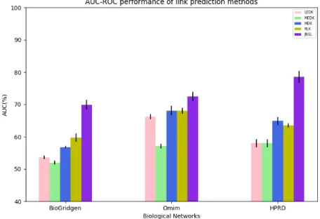
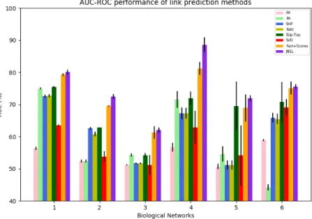
The second contribution aims at dealing with the graph sparsity problem. When working with sparse graphs, i.e graphs with a high number of missing links, the available information is not efficient to learn effectively. An idea to overcome this problem is to use link enrichment to enrich information for graphs. However, the performance of a link enrichment strongly depends on the adopted link prediction method. Therefore, we propose an effective link prediction method (JNSL). In this method, first, each link is represented as a joint neighborhood subgraphs. Then link prediction is considered as a binary classification. We empirically show that the proposed link prediction outperforms various other methods. Besides, we also present a method to boost the performance of diffusion-based kernels, which are most popularly used, by coupling kernel methods with link enrichment. Experimental results prove that the performances of diffusion-based graph node kernels are considerably improved by using link enrichment.
The last contribution proposes a general kernel-based framework for graph integration that we name Graph-one. Graph-one is designed to
over-it is a scalable and efficient framework. Besides, over-it is able to deal wover-ith unbanlanced settings where the number of positive and negative instances are much different. Numerous variations of Graph-one are evaluated in dis-ease gene prioritization context. The results from experiments illustrate the power of the proposed framework. Precisely, Graph-one shows better per-formance than various methods. Moreover, Graph-one with data integration gets higher results than it with any single data source. It presents the ef-fectiveness of Graph-one in exploiting the complementary property of graph integration.
1 Introduction 1
1.1 Why graph-based biological data integration? . . . 2
1.2 Kernel methods for graph-based data integration and challenges 3 1.2.1 Definition of node similarity measure . . . 3
1.2.2 Graph sparsity . . . 4
1.2.3 Scalability and efficiency . . . 4
1.2.4 Data integration methods . . . 4
1.3 Contributions . . . 4 1.4 Thesis roadmap . . . 6 1.5 List of publications . . . 6 2 Background 9 2.1 Machine learning . . . 9 2.2 Kernel methods . . . 11 2.3 Kernel functions . . . 12 2.4 Kernel machines . . . 15
2.4.1 Kernel Perceptron algorithm . . . 15
2.4.2 Support Vector Machine . . . 16
2.5 Kernels on graphs . . . 18
2.5.1 Graph kernels . . . 21
2.5.1.1 Product graph kernel . . . 21
2.5.1.2 Shortest path kernels . . . 21
2.5.1.3 Weisfeiler-Lehman kernels. . . 22
2.5.1.4 The neighborhood subgraph pairwise dis-tance kernel . . . 23
2.5.2 Graph node kernels. . . 23
2.5.2.4 Regularized Laplacian kernel . . . 25
2.6 Disease gene prioritization . . . 26
2.7 Biological datasets . . . 28
2.8 Link prediction . . . 29
2.9 Biological data integration . . . 31
2.10 Multiple kernel learning . . . 32
3 Conjunctive Disjunctive Graph Node Kernel 35 3.1 Motivation . . . 35
3.2 A new graph node kernel . . . 36
3.2.1 Network decomposition . . . 37
3.2.2 The conjunctive disjunctive node kernel . . . 38
3.2.3 Additional node information . . . 40
3.2.4 Hyper-parameter space . . . 41
3.3 Graph node labeling . . . 42
3.4 Empirical evaluation . . . 43
3.4.1 Experimental settings and evaluation methods . . . . 43
3.4.2 Model selection . . . 45
3.5 Results and discussion . . . 45
3.5.1 Degree distribution dependency analysis . . . 46
3.5.2 Sensitivity analysis for hyper-parameters. . . 47
3.6 Summary . . . 49
4 Solutions for Graph Sparsity 53 4.1 Motivation . . . 53
4.2 Joint neighborhood subgraphs link prediction method . . . . 54
4.2.1 Link encoding as subgraphs union . . . 54
4.2.2 Joint neighborhood subgraphs link prediction . . . 55
4.2.3 Empirical evaluation . . . 56
4.2.4 Results and discussion . . . 59
4.2.5 Summary . . . 59
4.3 Link enrichment for diffusion-based graph node kernels . . . . 59
4.3.1 Method . . . 60
4.3.2 Empirical evaluation . . . 61
4.3.3 Results and discussion . . . 62
Approaches 67
5.1 Graph-one: a general kernel-based framework for graph-based
data integration. . . 68
5.1.1 Graph-one flow . . . 68
5.1.2 Scalable unbalanced multiple kernel learning: UEasyMKL . . . 69
5.2 Graph-one for disease gene prioritization . . . 73
5.2.1 Graph-one variations for disease gene prioritization . . 73
5.2.2 Experiments and results . . . 75
5.2.3 Discussion . . . 79
5.3 Summary . . . 86
6 Conclusion and Future Work 89 6.1 Graph node measure definition . . . 89
6.2 Graph sparsity . . . 90
6.3 Graph-one: an efficient, scablable framework for graph-based integration. . . 91
6.4 Future work . . . 92
6.4.1 Graph side information . . . 92
6.4.2 Graph combination . . . 92
6.4.3 Applications . . . 92
Appendices 107 A Conjunctive Disjunctive Graph Node Kernel 109 B Solutions for Graph Sparsity 113 B.1 Joint neighborhood subgraphs link prediction . . . 113
B.2 Link enrichment for diffusion-based graph node kernels . . . . 115
C Graph-based Data Integration
Chapter 1
Introduction
The release of advanced technologies is one of the main reasons for the revolution in various scientific research fields. In Biological and Medical domain, modern technologies are making it not only easier but also more economical than ever to undertake experiments and creating applications. As a consequence, a vast amount of biological data in terms of volume and type is generated through scientific experiments, published literatures, high-throughput experiment technologies, and computational analysis. This huge quantity of data are saved as biological datasets and made discoverable through web browsers, application programming interfaces, scalable search technology and extensive cross-referencing between databases. Biological databases normally contain information about gene function, structure, lo-calization, clinical effects of mutations and similarities of biological sequences and structures.
The abundance of biological data, on the one hand, creates a golden chance for biologists to extract useful information. However, it, on the other hand, poses the challenge for scientists to wisely and effectively ex-tract knowledge from such amount of data that normally cannot be done without the help of automated learning systems. Hence, the task of devel-oping high performance learning systems, which help sciencists to form and assess hypotheses, plays an important role in the development of biology and medicine.
Figure 1.1: Yeast protein interaction network [2].
1.1
Why graph-based biological data integration?
Biological knowledge is distributed among general and specialized sources, such as gene expression, protein interaction, gene ontology, etc. It is common that information of a biological phenomenon is encoded over various hetero-geneous sources. Each source captures different aspects of the phenomenon. The distribution of information over sources provides us an unprecedented opportunity to understand the phenomenon from multiple angles.
Therefore, the idea of data integration which allows multiple sources of information to be treated in a unified way can in priciple lead to an im-provement of biological learning systems, i.e. systems that process with biological data. Despite the fact that data integration is a promising solu-tion, it poses a challenge for machine learning experts and data scientists to find out optimal solutions for combining multiple sources in a big space of solutions.
Relations between entities encoded in biological sources can be natu-rally represented in form of graphs (networks) whose vertices describe for biological entities and links characterize the relations between entities. An
example is the protein-protein interaction network (Figure 1.1) where each vertex represents a protein and a link connecting two vertices if they inter-act. Graph theory provides a mathematical abstraction for the description of such relationships. Thus, using graphs to represent for biological data al-lows us toi) access to a principled and solid mathematical framework built for graphs that most scientists are familiar with, ii) develop concepts and tools which are independent of the concrete applications. By using a graph presentation, the problem of biological data integration now can be con-verted into graph-based data integration. The final representation of data obtained by integration is used as input for the construction of inference systems (graph-based learning systems).
1.2
Kernel methods for graph-based data
integra-tion and challenges
Kernel methods whose best known member is support vector machine (SVM) [28], has emerged as one of the most famous and powerful frameworks in ma-chine learning. Kernel methods with the use of kernels allow to decouple the representation of the data (via kernel function) from the specific learning algorithm. Kernel representation is flexible and efficient and it provides a principled framework that allows universal type of data to be represented, including images, graphs, vectors, strings, etc. As a consequence, kernel methods are the state-of-the-art learning technique for graph-based infer-ence systems. However, there are a number of challenges that need to be efficiently solved, if we desire to have high performance graph-based data integration learning systems. Following are the main challenges: definition of node similarity measure, graph sparsity, data integration method.
1.2.1 Definition of node similarity measure
In machine learning, one of the main factors which impacts on the perfor-mance of learning systems is the definition of example similarity measure. In our context, large-scale graph-based inference systems, examples are nodes of graphs. Hence, it is necessary to have a good definition of node similar-ity measure. Node similarsimilar-ity is normally measured by graph node kernels. However, there is not a clear way to define a graph node kernel which can be efficiently applied to a wide range of graphs.
1.2.2 Graph sparsity
The input of a graph-based data integration system is a set of graphs which often contain sparse graphs whose number of links is much less than the number of possible links. This is typically due to the lack of information. For instance, in the disease gene network, links connecting genes are formed when genes are involved in the same diseases. However, new genes associated to a certain disease could be discovered over time. This means that new links could be added into the networks over time. At a given time, a number of discovered links can be very limited, so discovered links cause the sparsity problem. When working with sparse graphs, systems encounter difficulties in performing an effective training since not enough information is available to correctly learn the target function. As a consequence, an effective solution helping to overcome the sparsity problem is crucial and needs to be proposed.
1.2.3 Scalability and efficiency
Given an adopted learning algorithm, the complexity of a large-scale graph-based data integration learning system incurs with the growth of the input graph set. In other words, the complexity of a graph-based learning system strongly depends on the size and the number of graphs used as its input. Therefore, scalability is an important property that a graph-based learning system is supposed to possess. It allows systems to run in reasonable time and with a reasonable memory consumption.
1.2.4 Data integration methods
Information encoded in multiple sources (graphs) provide complementary views of the phenomenon of interest. Combining information from collective sources helps to form a complete picture of the phenomenon or problem at hand. Nonetheless, the search for efficient and scalable integration methods that allow to improve the performance of the learning system with respect to the same system where a single source of information is used, is normally expensive.
1.3
Contributions
The contributions of the thesis focus on solutions to overcome the challenges faced when working with large-scale graph-based biological data integration.
The first contribution considers the problem of defining an effective node similarity measure by introducing a novel graph node kernel, named conjunctive disjunctive node kernel (CDNK). Most existing graph node kernels are based on a notion of information diffusion which can be applied to dense networks with high values of average node degree. However, a drawback of these approaches is their relatively low discriminative capacity. This is in part due to the fact that information is processed in an additive and independent fashion which prevents them from accurately modeling the configuration of each node context. To address this issue, we propose to employ a decompositional graph kernel technique in which the similarity function between graphs can be formed by decomposing each graph into subgraphs and by devising a valid local kernel between the subgraphs. In CDNK, to exploit its higher discriminative capacity, first the network is decomposed into a collection of connected sparse graphs and then a suitable kernel is developed.
The second contribution aims to propose solutions for graph sparsity problem. Graph data integration methods take graphs as the input. However, if graphs are sparse, the information is not efficient to learn. It leads to low performance of graph data integration methods. A solution is to enrich information on graphs by employing link enrichment. Neverthe-less, the performance of a link enrichment method strongly relies on the adopted link prediction. Therefore, we introduce a link prediction method, which is adopted later on for link enrichment with the aim of solving the problem of graph sparsity. We get the motivation from the current link prediction methods that do not effectively exploit the contextual information available in the neighborhood of each edge. In our method, we propose to cast the problem as a binary classification task over the union of the pairs of subgraphs located at the endpoints of each edge. We model the classification task using a support vector machine endowed with an efficient graph kernel and achieve state-of-the-art results on several benchmark datasets. Moreover, we also proposes a method that boosts the performance of diffusion-based kernels when working with sparse graphs by tackling them with link enrichment methods. In particular, given a sparse graph, our proposed method consists of two phases. In the first phase, a link prediction method is employed to rank unobserved links based on their probabilities to be related to missing links. The top links in the ranking are then added into the graph. In the second phase, diffusion-based graph node kernels are applied to the graph obtained from the first phase to compute
the kernel matrix.
The last contribution presents a general framework, named Graph-one, for graph integration. Graph-one is an efficient and scalable kernel-based framework which is able to deal with the unbalanced settings. Therefore, can overcome the challenges for large-scale graph-based integration. We evaluate Graph-one by introducing its different variations (Scuba, PLC, DIGI) in the context of disease gene prioritization. Experimental results illustrate that
i) Graph-one outperforms various methods, and ii) Graph-one with data integration shows better performance than it with any single data source.
1.4
Thesis roadmap
The thesis is organized as follows:
Chapter 2 presents preliminary concepts, notations and comprehensive review of the state-of-the-art in the field.
Chapter 3 proposes an effective convolutional graph node kernel, Conjunctive Disjunctive Graph Node Kernel (CDNK).
Chapter 4 introduces solutions to solve the graph sparsity problem: a novel link prediction method (JNSL) and a method to boost the perfor-mance of diffusion-based kernels when working with sparse graphs.
Chapter 5 describes a general kernel-based framework, Graph-one for large-scale graph-based data integration.
Chapter 6 summarizes the contributions of the thesis and discusses the directions for future work.
1.5
List of publications
1. Dinh Tran Van, Alessandro Sperduti and Fabrizio Costa, Conjunctive Disjunctive Node Kernel, the 25th European Symposium on Artificial Neural Networks, Computational Intelligence and Machine Learning, Bruges (Belgium), 26-28 April, 2017, ISBN 978-287587039-1.
2. Dinh Tran Van, Alessandro Sperduti and Fabrizio Costa, Link En-richment for Diffusion-based Graph Node Kernels, the 26th
Interna-tional Conference on Artificial Neural Networks, Alghero, Italy, 11-15, Steptember, 2017.
3. Dinh Tran Van, Alessandro Sperduti and Fabrizio Costa, Joint Neigh-borhood Subgraphs Link Prediction, the 24th International Confer-ence on Neural Information Processing, Guangzhou, China, November 1418, 2017.
4. Guido Zampieri, Dinh Van Tran, Michele Donini, Nicol Navarin, Fabio Aiolli, Alessandro Sperduti and Giorgio Valle, Scuba: scalable kernel-based gene prioritization, BMC Bioinformatics, DOI 10.1186/s12859-018-2025-5, 2018.
5. Dinh Tran Van, Alessandro Sperduti and Fabrizio Costa , Conjunctive Disjunctive Node Kernel, Neurocomputing, 2018.
Chapter 2
Background
In this chapter, we describe preliminary knowledge and notaions and com-prehensive review of the state-of-the-art in the field used for the remaining parts of the thesis. We aim to make it easy for readers to follow the expo-sition of its original contributions.
2.1
Machine learning
Recently, machine learning has become a must-know term not only in academia but also in daily life due to the popularity of it’s applications in various fields. Machine learning can be considered as a branch of Artifi-cial Intelligence which aims at providing systems the ability to automatically adapt to their environment and learn from experience without being explic-itly programmed. According to [64], machine learning is formally defined as:
Definition 2.1.1. A computer program is said to learn from experience E
with respect to some task T and some performance measure P if its perfor-mance onT, as measured by P, improves with experience E.
We denoteDas a set of training examples which come from some gener-ally unknown probability distribution. D is resulted from any observation, measurement or recording apparatus for a certain domain A machine lean-ring technique aims at exploiting D to build a general model about the example space. This model is then used to produce sufficiently accurate predictions in unseen examples.
Machine learning algorithms can be classified into three paradigms: su-pervised learning, unsusu-pervised learning and reinforcement learning. Su-pervised learning is the machine learning task of inferring a function from labeled training examples in which each example is a pair consisting of an entity and a desired output value (label). A supervised learning algorithm analyzes the training data and forms an inferred function, which is used for mapping unseen examples. Unsupervised learning is a machine learning task that models a set of inputs where labeled examples are not available. Re-inforcement Learning aims at designing machines and software agents that can automatically determine the ideal behaviour within a specific context, in order to maximize its performance. Simple reward feedback is required for the agent to learn its behaviour; this is known as the reinforcement signal. In this thesis, we focus on supervised learning scenario.
We consider a training setD generated by an unknown probability dis-tributionP,D={(x1, y1),(x2, y2), . . . ,(xn, yn)}wherexi∈Xare instances andyi ∈Yare labels. The relations betweenxi andyi are defined by a true
function (target function)f :X7−→Y. What we desire to do is to learn the functionf. However, the only information we can access is from the training set. Therefore, a supervised learning method aims at estimating a function
h based on D to be as close to f as possible. Depending on the domain of Y, we can further group supervised learning into the following sub-groups:
• ifY⊆R, the problem is called regression;
• if|Y|= 2, we have a binary classification problem;
• if|Y|=n withn >2, we have multi-class classification problem. Besides, a multi-class learning is called multi-label if examples have more than one label associated with. It is worth highlighting that there is normally more than one possible choice forh. We refer each choice ofhas a hypothesis or model and the set of all possible h as hypothesis space, H. The goal of the learning process is to find the final hypothesis that best approximates the unknown target function. In order to measure the difference between a hypothesis and the target function, the risk function is used:
R(h) =
Z
X×Y
L(h(x), y)dP(x, y), (2.1) where L is a loss function that measures the classification error of h. An example of the loss function for classification can be defined as:
The optimal hypothesis is the one which minimizes the risk and it is the solution of the following optimization problem:
h∗ = arg min
h∈H
R(h). (2.2)
Unfortunately, it is impossible to directly solve the optimization problem described in eq. 2.1 since the probability distribution P in the true loss function presented in eq. 2.2 is an unknown function and we only have access to a finite training set D. In this case, an alternative approach is to use the empirical loss instead of the true loss function. The empirical loss function is defined over the training set as follows:
Remp(h) = 1 n n X i=1 |h(xi)−yi|, (2.3)
where n is the number of traning examples. However, in order to use
Remp(h), we need to guarantee that the value of Remp(h) converges to the value of R(h).
In the typical statistical learning framework, every data instance is em-bedded in a suitable space. However, most real world data has no natural representation as vectorial forms. Kernel methods have been successful in various learning tasks on data represented by vectors, but structured forms, including graphs. In this thesis, we are interested in investigating graph-based integration methods. Therefore, in the next section we describe Ker-nel methods.
2.2
Kernel methods
In classical machine learning techniques, each data instance is mapped to a point in the feature space,x∈X−→φ(x)∈F. Then a model is constructed from the training set and is used to predict for unseen data. Although these approaches have sucessfully applied in some cases, they share two common limitations: i) If the dimension of the feature space is high, it leads to high complexity algorithms. ii) It is difficult or even impossible in some cases to find the mapping.
Kernel methods have been proposed and shown the state-of-the-art re-sults in many cases of various fields. SVM [28] is a typical example of Kernel methods. Unlike the presentation of data in traditional machine learning, in kernel methods, data instances are not individually represented in the feature space, instead they are represented by similarity measures between
pairs of instance images, which are computed by using dot product. The dot product of instance image pairs can be computed through input instances only by kernel functions. Kernel functions enable kernel methods to operate in a high-dimensional, implicit feature space without ever computing the coordinates of the data in that space, but rather by simply computing the inner products between the images of all pairs of data instances in the fea-ture space. This operation is often computationally cheaper than the explicit computation of the coordinates. Kernel functions have been introduced for sequence data, graphs, text, images, as well as vectors. A kernel methods can be modularized into two components: the design of a specific kernel function and the design of a general learning algorithm (kernel machine).
2.3
Kernel functions
In kernel methods, the definition of kernel functions is independent from the definition of general learning algorithms. Therefore, a given generl learning algorithm can go with any kinds of kernel functions. A number of kernel functions have been proposed for different types of data. In this section, we first formally define what is a kernel function. We then introduce some kernels defined on graphs that later on are used in our experiments.
Definition 2.3.1. Given a set of entities X, a function k:X×X7−→R is
called a kernel onX×X iff kis
• symmetric: it meansk(x1, x2) =k(x2, x1), where x1, x2 ∈X.
• positive semi-definite: that is PN
i=1
PN
j=1cicjk(xi, xj) ≥ 0 for any
N >0, ci, cj ∈R, and xi, xj ∈X.
The similarity measures computed by a kernel over a set of in-put instances can be represented in a matrix, called Gram matrix, K. K
is symmetric and positive semi-definite, i.e. its eigenvalues are non-negative.
K = k(x1, x1) k(x1, x2) k(x1, x3) . . . k(x1, xn) k(x2, x1) k(x2, x2) k(x2, x3) . . . k(x2, xn) .. . ... ... . .. ... k(xn, x1) k(xn, x2) k(xn, x3) . . . k(xn, xn) .
The simplist kernel is Linear kernel which is defined on vectors,X⊆Rn:
Figure 2.1: The kernel trick transforms the data in a feature space where the instances from the two classes may be linearly separable.
where x1, x2 ∈ X. This kernel suggests a systematic way to define kernels. Given a general set of representations of entities X, we first project each element inXinto a vector space, called feature space, x∈X−→φ(x)∈Rm such that m n. This is due to that fact that it is easier to find a linear decision line in higer dimensional space (m). Next, we define a kernel as:
k(x1, x2) =φ(x1)|φ(x2) (2.5) Interestingly, any kernel defined onX, there exists a Hilbert space,F, and a mappingφ:X−→Fsuch that k(x1, x2) =φ(x1)|φ(x2), where x1, x2 ∈X.
There are two problems we might face with if we would like to explic-itly embed objects into a vector space. i) if m is too big, we face with the high computation. ii) if data instances are in the structured forms (strings, graphs, trees, etc), we need to transform them into vectorial forms. One way is to decompose each instance into a set of sub-structures which are consid-ered as elements of vectors. However, in general, there is not a clear way to projecct instacnes in structured forms into feature space without loos-ing much information. These limitations are effectively solved by usloos-ing the so called Kernel trick. The kernel trick (see Figure 2.1 for an illustration) avoids the explicit mapping. Instead, it allows the operations (dot product) between vectors in the feature space to be done by computing in the input space. It is worth to notice that a kernel is considered as a similarity (prox-imity) measure since its value computed for two objects is proportional to their similarity.
Most kernels are defined on vectorial form of data among which Basis Function kernel (RBF) [92] is the most used one. However, real-world data often cannot be represented in the vectorial form without loosing important information. Therefore, a high number of kernels are proposed to deal with structured data, including trees, graphs, etc.
Convolution kernels
On the development of kernels for structured data, R-convolution kernels originally proposed in [43] and a generalization of the framework is proposed in [80] can be considered as one of the most important frameworks. The basic idea of convolution kernels is that the semantics of composite entities can often be captured by a relation R between the entity and its parts. The kernel between entities is then made up from kernels defined on different parts.
Letx be a composite structure whose x1, x2, . . . , xN = ˆx are parts ofx,
such thatx∈X, xi ∈Xi, i= 1, N andX,X1,X2, . . . ,XN are non-empty and
separable metric spaces. We define a relationR(ˆx, x) onX1×X2×. . .×XN×X is true iffx1, x2, . . . , xN are the parts ofx. We denote withR−1 the inverse
relation ofR and it is defined asR−1(x) ={xˆ|R(ˆx, x)}.
If there exists kernelki defined on Xi, the similarity betweenx, y∈Xis defined onS×S, whereS={x|R−1(x)6=∅}, as:
K(x, y) = X ˆ x∈R1(x),yˆ∈R1(y) N Y i=1 ki(xi, yi) (2.6)
K is referred as finite convolution, if R is finite. The zero expansion of K
toX×Xis called R-convolution and it is denoted as K1? K2? . . . KN(x, y).
Theorem 1. IfK1, K2, . . . , KN are kernels onX1,X2, . . . ,XN, respectively,
andR is a finite relation onX1×X2×. . .×XN, then K1? K2? . . . KN(x, y)
is a kernel on X×X. Constructing kernels
Kernels can be constructed from predefined kernels. Let k1, k2 be kernels over X×X, X ⊆ Rn, α1, α2 ∈ R+, f(.) a real valued function on X, φ a mappingX 7−→RN, k3 a kernel over RN ×RN, and Bn×n is a symmetric,
positive demi-definite. The following functions are kernels:
• k(x, y) =α1k1(x, y) +α2k2(x, y)
• k(x, y) =k1(x, y)k2(x, y)
• k(x, y) =f(x)f(y)
• k(x, y) =k3(φ(x), φ(y))
The proof of above kernels and other ways to form kernels from pre-defined kernels are presented in [76].
2.4
Kernel machines
In machine learning, there is a high number of techniques which aim at finding linear relations in datasets which are represented in vectorical forms. However, in many cases, the expected linear relations do not exist. A solu-tion to overcome these situasolu-tions is to first explicitly perform a non-linear transformation of input instances into a higher dimensional space and then search for linear relations in that space. Unlike traditional machine meth-ods, kernel methods with the use of kernel functions are able to operate in a high-dimensional space without ever computing the coordinates of the data in that space, but rather by simply computing the inner products between the images of all pairs of data in the feature space. This operation is often computationally cheaper than the explicit computation of the coordinates.
A number of traditional machine learning methods exploiting dot prod-ucts for computing can be turned into versions that exploit kernels, i.e. replacing the dot products with kernel computations. Therefore, their ex-pressive power are increased. Examples are Kernel Perceptron, Support Vector Machines (SVM), Kernel Gaussian Processes, Kernel Principal Com-ponents Analysis (PCA), etc. In the next sections, we will introduce in detail two famous algorithms: Kernel Perceptron and SVM. For the simplicity, we describe these algorithms in the context of binary classification.
2.4.1 Kernel Perceptron algorithm
Perceptron [13] is an old, online leanring algorithm which is based on error-driven learning. It desires to learn a hyper-plane,w|x+b= 0 orw|x= 0 for simplicity, to separate positive instances from negative ones in the training set. It is then used to predict a label for each unseen instance,x, through the
sgn function. Ifw|x≥0, the output of the Perceptron is ˆy =sgn(w|x) = 1, otherwise ˆy=−1.
Perceptron works by first initilizing values for weight vector, w. It then iteratively improves the performance by updating the weight vector when-ever a misclassification is found in the training set. Consider yi and ˆyi as
the true label and the predicted label for xi, respectively, if yi 6= ˆyi, w is
updated as follows:
whereα∈(0,1] is the learning rate. Suppose thatn misclassified examples are observed, the weight vectorw can be expressed as:
w=
n
X
i=1
αyixi. (2.7)
The update of the weights is done if the current input is not misclassified. This algorithm guarantees that a linear separation is found if it exists. When the linear separation does not exist, a possible solution is to embed input data into a higher dimensional space. By virtue of doing so, there is a higher chance to have linear separation. However, when the algorithm operates in a high dimensional space, it faces with the high complexity. As a conse-quence, Kernel Perceptron method [14], an extension of original Perceptron, is proposed to cope with high dimensional spaces.
Suppose thatφ(x) is the image ofx in feature space. We rewrite eq.2.7
to compute the weight vector in the feature space as:
w= n X i=1 αyiφ(xi). Then we get sgn(w|φ(x)) = n X i=1 αyiφ(xi)|φ(xj).
One limitation of both Perceptron and Kernel Perceptron method is that they are not able to find the optimal linear separation. Normally, among all possible linear separations, there might exist some which show bad predicting ability for unseen data. In the next section, we describe SVM, a kernel method, which aims at finding an optimal hyperplane to separate positive instances from negative ones.
2.4.2 Support Vector Machine
The original Support Vector Machine is a linear classifier and it was invented by Vladimir N. Vapnik [90]. SVM became popular when Vladimir et al introduced in [18] a way to create nonlinear classifiers by employing the notion of kernel trick. In particular, a SVM searches for an optimal hyper-plane in the feature space,H, through operations in input space only.
Given a set of training examples {(x1, y1),(x2, y2), . . . ,(xN, yN)} in
training set are linearly separable. SVM tries to learn a decision function
fw,b(x) =w|x+b, (2.8)
such thatfw,b(xi)yi≥0, b∈R is the bias, andw∈Rn is the norm vector. This function forms two half-spaces of instances: h+ ={x :f(x) ≥1}
and h− ={x :f(x) ≤ −1}. The distance between these two half-spaces is referred as margin and equal to kw2k.
The optimal hyperplane is the solution of the below quadratic optimiza-tion problem (primal form):
maximize w,b 1 kwk subject to yi(w|xi+b)≥1. (2.9) It is equivalent to minimize w,b 1 2kwk 2 subject to yi(w|xi+ 1)≥1. (2.10)
It is easier to use the dual form that can be obtained by the introduction of Lagrangian multipliers. Since the the optimization is convex, the solution of dual form is the same as primal form. The resulting Lagrange multiplier equation we desire to optimize is
L(w, b, α) = 1 2kwk 2− N X i=1 αi[yi(w|xi+b)−1], (2.11)
where αi ≥ 0 are Lagrange multipliers. Solving Lagrangian optimization
eq. 2.11, we obtain values for w, b and α which determin a unique hyper-plane. Thexiscorresponding to αiswhich differ from 0 are called support
vectors.
The formula of the hyperplane decision function eq. 2.8can be rewritten as: f(x) = N X i=1 yiαix|xi+b. (2.12)
In the case that the training set is not linearly separable, we can apply the kernel trick to let SVM to operate in possibly higher dimensional Hilbert space. By doing so, we hope in a higher dimensional space, there exist a hyperplane that separates images of positive instances from the negative
ones. f(x) = N X i=1 yiαiφ(x)|φ(xi) +b. (2.13)
There are usually very fewαiswhich are equal to 0. Therefore, it requires
a low computation to predict for unseen examples.
In practice, there are two problems that we need to take into account. First, in many cases, the separating hyperplane does not exist in the feature space due to the high level of noise in data. Second, the learning function is so complex that it not only fits instances, but it also fits the noise. Therefore, the function is able to classify the training set, but it fails to generalize for unseen data. The latter problem is called overfitting. In order to solve such problems, a solution one may think is to allow examples to violate eq. ??.
A soft margin SVM is introduced in which a trade-off between the mis-takes on the training set and the complexity of the hypothesis is defined. The optimization eq. 2.10 is modified by introducing slack variablesξi:
minimize w,b,ξ 1 2kwk 2+C N X i=1 ξi subject to yi(w|xi+ 1)≥1−ξi, (2.14)
where ξi ≥ 0 and C is a constant which determines the trade-off between
margin maximazation and the training error minimization.
2.5
Kernels on graphs
Canonical machine learning methods take vectorial data, data that are rep-resented by vectors of features, as their input. However, there are many fields where data are not naturally represented by vectors, but by structured forms in which graph is one of the most popular representation. Therefore, the task of developing methods which are able to learn from structured data in general or graphs in particular is very important. In this thesis, we focus on graphs, a special type of structured data representation. An example of data that can be represented by graph is the genetic network, where each node represents a gene and each link is formed between two genes, if they encode common protein(s). Another example is the social network whose nodes are users and links depict friendship between users. Systems that deal with problems where data are naturally represented as graphs are called graph-based systems.
One of the key points that determines the performance of a learning system is the similarity measure definition. In our context is the similarity measure definition between graphs. An idea is to find ways that map graphs into vectorial forms: X7−→Rn, and then employ similarity functions defined on vectors. However, the task of designing these mappings, which are able to encapsulate all information in a vectorial form, is a difficult task since they need to:
• map isomorphic graphs into the same vector;
• non-isomorphic graphs into different vectors;
• be efficient in terms of time computation and memory consumption. Recently, kernel methods with the use of kernel functions have emerged as one of the most powerful frameworks in machine learning. Kernel func-tions are considered as similarity funcfunc-tions which can be defined on any type of data representation. Therefore, the similarity measures defined on graphs mostly are kernels. There are two groups of kernels defined on graphs. The first group consists of kernels that aim at measuring the similalrities between graphs and they are referred as graph kernels. To have an overview of graph kernels, we recommend to readers a survey on graph kernels presented in [93]. The second one includes kernels which intend to measure the similari-ties between nodes inside graphs and are called graph node kernels or node kernels in short. For analysis of different graph node kernels, we suggest to read the work proposed in [34].
In the following, we first give formal definitions and notations related to a graph. We then give an overview of graph kernels followed graph node kernels.
Definition 2.5.1. A graph is a structure G = (V,E,Ln,Le) where V =
{v1, v2, . . . , vn} is the node (vertex) set,E={(vi, vj)} ⊆(V×V) is the link (edge) set andLn,Le are the node and edge function, respectively.
Definition 2.5.2. An undirected graph is a graph in which edges have no orientation. The edge(u, v) is identical to the edge (v, u), i.e. they are not ordered pairs, but sets {u, v} (or 2-multisets) of vertices. The maximum number of edges in an undirected graph without a loop isn×(n−1)/2.
Definition 2.5.3. An adjacency matrix A is a symmetric matrix used to characterize the direct links between vertices vi and vj in the graph. Any
entry Aij is equal to wij when there exists a link connecting vi and vj, and
Definition 2.5.4. The Laplacian matrix L is defined as L=D−A, where
Dis the diagonal matrix with non-null entries equal to the summation over the corresponding row of the adjacency matrix, i.e. Dii=PjAij.
Definition 2.5.5. The transition matrix of a graph G, denoted as P, is a matrix in which each elementPij =Aij/PiAij is the probability of stepping
on nodej from node i.
We define thedistance D(u, v) between two nodesuandv, as the number of edges on shortest path between them. Theneighborhood of a nodeuwith radius r, Nr(u) = {v | D(u, v) ≤ r}, is the set of nodes at distance no
greater than r from u. The corresponding neighborhood subgraph Nu r is
the subgraph induced by the neighborhood (i.e. considering all the edges with endpoints in Nr(u)). The degree of a node u, deg(u) = |N1u|, is the cardinality of its neighborhood. The maximum node degree in the graphG
is denoted bydeg(G).
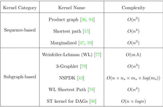
Table 2.1: Summary of some popular graph kernels. h: the hight, ns, ms:
number of nodes, edges in subgraphs, respectively.
Kernel Category Kernel Name Complexity
Sequence-based Product graph [36,94] O(n3) Shortest path [15] O(n4) Marginalized [47,59] O(n3) Subgraph-based Weisfeiler-Lehman (WL) [77] O(m.h) 3-Graphlet [79] O(n3) NSPDK [43] O(n×ns×ms×log(ms)) WL Shortest Path [78] O(n4) ST kernel for DAGs [30] O(n×logn)
2.5.1 Graph kernels
The task of designing effcient and expressive graph kernels play an important role in the development of graph-based predictive systems. One of the first systematic works that strongly impacts on the development of research on graph kernels is convolution or decomposition kernel [43] (see Section 2.3). Existing graph kernels are decompositional kernels and can be classified into two categories: sequence-based graph kernels and subgraph-based graph kernels. The sequence-based graph kernels decompose graphs into “parts” in sequence-based forms, such as paths and walks; meanwhile, the subgraph-based graph kernels dissolve graphs into subgraphs. Table2.1is a summary of some popular graph kernels. Following, we describe some of kernels in each category.
2.5.1.1 Product graph kernel
Product graph kernel was originaly proposed in [36] with the aim to measure the similarity between two labeled graphs by counting their common walks. To compute the similarity between two graphs (factor graphs), first a graph, called direct product graph, is constructed from two factor graphs. Then the similarity is computed based on the obtained graph.
Formally, we consider two factor graphs G1 and G2 and Ln1,Ln2, Le1,
Le2 as the node and edge labeling functions of G1 andG2, respectively. We define the direct product graph of G1,G2 as a graphG× = (V×, E×) where
• V× ={(u, v) :u∈V(G1)∧v∈V(G2)∧ Ln1(u) =Ln2(v)};
• E×={((u, v),(u0, v0))∈V××V× : (u, v)∈E(G1)∧(u0, v0)∈E(G2) ∧ Le1((u, v)) =Le2((u0, v0))}.
Givenλ1, λ2, . . .(λi ∈R, λi ≥0, ∀i∈N), the direct product kernel is defined as follows k(G1, G2) = |V×| X i,j=1 "∞ X n=0 λnAn× # ij , (2.15)
if the limit exists, in whichA×is the adjacency matrix of the direct product
graphG×. The computation of this limit is high,O(n6). There are different
modifications of this kernel that can be more efficient to compute, such as the method proposed in [94] that has complexity of O(n3).
2.5.1.2 Shortest path kernels
The simple idea behind shortest path kernels is that they consider the com-mon shortest paths between two graphs to measure their similarity.
Al-though the computation of shortest paths in a graph can be computed in polinomial time, taking into account shortest paths leads to some prob-lems. First, the shortest paths between two nodes normally are not unique and there has not been a way to deterministically choose one shortest path among others. Second, if we keep all shortest paths into account, it would lead to a NP-hard kernel. Although the shortest paths are not unique, the length of them is unique. As a consequence, a shortest path graph kernel is proposed in [15] with total runtime of O(n4).
Given two graphs G1, G2, we first construct their two corresponding shortest graphsGs1,Gs2, respectively. The shortest graph of a graph,G, is
a labeled graph defined asGs= (Vs, Es) where
• Vs=V(G);
• Es={(u, v) :u, v∈V(G)∧ |p(u, v)| ≥1} wherep(u, v) is the number
of shortest paths connectinguand v;
• Le((u, v)) =D(u, v).
We then define the shortest graph kernel forG1 andG2 as follows:
ks(G1, G2) = X (u1,v1)∈E(Gs1) X (u2,v2)∈E(Gs2) kwalk1 ((u1, v1),(u2, v2)), (2.16) wherek1
walk is a positive semi-definite kernel on 1-length walks.
2.5.1.3 Weisfeiler-Lehman kernels
The Weisfeiler-Lehman kernel framework is proposed in [78]. It is derived from the kernel proposed in [77]. The idea is to first decompose each graph into a sequence of graphs. Then the similarity between two graphsGandG0
is the summation of values computed by a given kernel defined on the two corresponding graph sequences, derived fromGandG0 by applying different labeling functions.
Formally, the Weisfeiler-Lehman graph sequence of a given graph
G= (V, E,L) up to the heighth is defined as:
{G0, G1, . . . , Gh}={(V, E,L0),(V, E,L1), . . . ,(V, E,Lh)},
whereG0=G,L0 =L,Lis (i= 1, h) are different labeling function on G.
Given two graphs G, G0 and a graph kernel k, the Weisfeiler-Lehman kernel,kW L is defined as:
kW L(G, G0) =k(G0, G 0 0) +k(G1, G 0 1) +. . .+k(Gh, G 0 h). (2.17)
2.5.1.4 The neighborhood subgraph pairwise distance kernel The NSPDK is an instance of convolution kernel [43] where given a graph
G∈ G and two rooted graphsAu, Bv, the relation Rr,d(Au, Bv, G) is trueiff
Au ∼=Nru is (up to isomorphism ∼=) a neighborhood subgraph of radiusr of
Gand so isBv ∼=Nrv, with roots at distanceD(u, v) =d(see Figure2.2). We
denote withR−1 the inverse relation that returns all pairs of neighborhoods of radius r at distance din G, Rr,d−1(G) ={Au, Bv|Rr,d(Au, Bv, G) =true}.
The kernelκr,d overG × G, counts the number of such fragments in common
in two input graphs:
κr,d(G, G 0 ) = X Au,Bv ∈ R−r,d1(G) A0u0,B0v0 ∈ R−r,d1(G0) 1Au∼=A0 u0 ·1Bv∼=B0 v0, (2.18)
where1A∼=B is theexact matching function that returns 1 ifAis isomorphic
toB and 0 otherwise. Finally, the NSPDK is defined as
K(G, G0) =X
r
X
d
κr,d(G, G0), (2.19)
where for efficiency reasons, the values of r and d are upper bounded to a given maximalr∗ and d∗, respectively.
u v u
v
d=3
Figure 2.2: Example of a pairwise neighborhood subgraphs rooted atuwith radiusr= 1 and distance d= 3.
2.5.2 Graph node kernels
Different from graph kernels which aim at measuring similarities between graphs, graph node kernels intend to measure similarities between nodes in graphs. The ideas behind graph node kernels are similar to graph ker-nels. Therefore, they can also be devided into sequence-based graph node kernels and subgraph-based graph node kernels. However, graph node ker-nels attempt to exploit the configuration concerning two nodes in the graph in order to define their similarity. Most available graph node kernels are sequence-based graph node kernels and they are based on the diffusion phe-nomenon. In other words, they consider paths connecting two given nodes
in order to form their similarity. Table 2.2 is a summary of some popular node graph kernels. In the following, we introduce some most used graph node kernels.
Table 2.2: Summary of some popular sequence-based graph node kernels. t
is a constant
Kernel Category Kernel Name Complexity
Sequence-based
LEDK [52] O(n2) MEDK [24] O(n2)
MDK [35] O(t×n2.373) RLK [22] O(n2.373)
2.5.2.1 Laplacian exponential diffusion kernel
One of the most well-known kernels for graphs is the Laplacian exponential diffusion kernelLEDK, as it is widely used for exploiting discrete structures in general and graphs in particular. On the basis of the heat diffusion dy-namics, Kondor and Lafferty proposedLEDKin [52]: imagine to initialize each vertex with a given amount of heat and let it flow through the edges until an arbitrary instant of time. The similarity between any vertex couple
vi,vj is the amount of heat starting fromvi and reachingvj within the given
time. Therefore, LEDK can capture the long range relationship between vertices of a graph to define the global similarities. Below is the formula to computeLEDKvalues:
K =e−βL =I−βL+βL 2
2! −. . . , (2.20) whereβis the diffusion parameter and is used to control the rate of diffusion and I is the identity matrix. Choosing a consistent value for β is very important: on the one side, ifβ is too small, the local information cannot be diffused effectively and, on the other side, if it is too large, the local information will be lost. LEDK is positive semi-definite as proved in [52]. The kernel requires to compute a matrix exponential which involvesO(n3)
operations using the Sylvester method, orO(n2) using the method proposed in [106].
2.5.2.2 Exponential diffusion kernel
In LEDK, the similarity values between high degree vertices are generally higher compared to those between low degree ones. Intuitively, the more paths connect two vertices, the more heat can flow between them. This could be problematic since peripheral nodes have unbalanced similarities with respect to central nodes. In order to make the strength of individual vertices comparable, a modified version of LEDKintroduced by Chen et al in [24] is called Markov exponential diffusion kernelMEDK and given by the following formula:
K =e−βM. (2.21)
The difference with respect to the Laplacian diffusion kernel is the replace-ment of Lby the matrix M = (D−A−nI)/nwheren is the total number of vertices in graph. The role of β is the same as for LEDK. MEDK also requires the matrix exponential, so it has the same complexity as LEDK.
2.5.2.3 Markov diffusion kernel
The original Markov diffusion kernel MDKintroduced by Fouss et al. [35] exploits the idea of diffusion distance, which is a measure of how similar the pattern of heat diffusion is among a pair of initialized nodes. In other words, it expresses how much nodes ”influence” each other in a similar fashion. If their diffusion ways are alike, the similarity will be high and, vice-versa, it will be low if they diffuse differently. This kernel is computed starting from the transition matrixPand by defining Z(t) = 1tPt
τ=1Pτ, as follows:
K=Z(t)Z>(t). (2.22) MDK computes t matrix multiplications, each one with a cost of approx-imately O(n2.373) by using the fastest algorithm [31, 81]. Therefore, its complexity is O(t×n2.373).
2.5.2.4 Regularized Laplacian kernel
Another popular graph node kernel function used in graph mining is the regularized Laplacian kernel RLK. This kernel function was introduced by Chebotarev and Shamis in [22] and represents a normalized version of the
random walk with a restart model. It is defined as follows: K = ∞ X n=0 βn(−L)n= (I +βL)−1, (2.23) where the parameter β is again the diffusion parameter. RLK counts the paths connecting two nodes on the graph induced by taking −L as the adjacency matrix, regardless of the path length. Thus, a non-zero value is assigned to any couple of nodes as long as they are connected by any indirect path. RLKremains a relatedness measure even when the diffusion factor is large, by virtue of the negative weights assigned to self-loops. The kernel RLK requires a matrix inversion, the same complexity as matrix multiplicationO(n2.373).
2.6
Disease gene prioritization
The identification of the genes underlying human diseases is a major goal in current molecular genetics research. Dramatic progresses have been made since the 1980s, when only a few DNA loci were known to be related to dis-ease phenotypes. Nowadays opportunities for the diagnosis and the design of new therapies are progressively growing, thanks to several technological advances and the application of statistical or mathematical techniques. For instance, positional cloning has allowed to map a vast portion of known Mendelian diseases to their causative genes [82, 19]. Despite the huge ad-vances, much remains to be discovered. On December 21st 2016, the Online Mendelian Inheritance in Man database (OMIM) registered 4,908 Mendelian phenotypes of known molecular basis and 1,483 Mendelian phenotypes of unknown molecular origin [4]. Moreover, 1,677 more phenotypes were sus-pected to be Mendelian. But it is among oligogenic and poligenic (and multifactorial) pathologies that the most remains to be elucidated: for the majority of them, only a few genetic loci are known [82,19].
Independently of the type of disease, the search of causative genes usually concerns a large number of suspects. It is therefore necessary to recognise the most promising candidates to submit to additional investigations, as experimental procedures are often expensive and time consuming. Gene prioritization is the task of ordering genes from the most promising to the least. In traditional genotype-phenotype mapping approaches - as well as in genome-wide association studies - the first step is the identification of the genomic region(s) wherein the genes of interest lie. Once the candidate re-gion is identified, the genes there residing are prioritized and finally analysed
for the presence of possible causative mutations [82]. More recently, in new generation sequencing studies this process is inverted as the first step is the identification of mutations, followed by prioritization and final validation [73]. Prioritization criteria are usually based on functional relationships, co-expression and other clues linking genes together. In general, all of them follow the “guilt-by-association” principle, i.e. disease genes are sought by looking for similarities to genes already associated to the pathology of in-terest [82].
In the last few years, computational techniques have been developed to aid researchers in this task, applying both statistics and machine learning [66]. Thanks to the advent of high-throughput technologies and new gener-ation sequencing, a huge amount of data is in fact available for this kind of investigations. In particular, computational methods are essential for
multi-omics data integration, that has been recognised as a valuable strategy for understanding genotype-phenotype relationships [72]. In fact, clues are often embedded in different data sources and only their combination leads to the emergence of informative patterns. Furthermore, incompleteness and noise of the single sources can be overcome by inference across multiple levels of knowledge.
Several popular algorithms for pattern analysis are based on kernels, which are mathematical transformations that permit to estimate the sim-ilarity among items (in our case genes) taking into account complex data relations [76]. Importantly, kernels provide a universal encoding for any kind of knowledge representation, e.g. vectors, trees or graphs. When data integration is required, a multiple kernel learning (MKL) strategy allows a data-driven weighting/selection of meaningful information [41]. The goal of MKL is indeed to learn optimal kernel combinations starting from a set of predefined kernels obtained by various data sources. Through MKL the issue of combining different data types is then solved by converting each dataset in a kernel matrix.
Numerous MKL approaches have been proposed for the integration of genomic data [96,16] and some of them have been applied to gene prioriti-zation [32,102,65,103]. De Bieet al formulated the problem as a one-class support vector machine (SVM) optimization task [32], while Mordelet and Vert tackled it through a biased SVM in a positive-unlabelled framework [65,20]. Recently, Zakeriet al proposed an approach for learning non-linear log-euclidean kernel combinations, showing that it can more effectively de-tect complementary biological information compared to linear combinations-based approaches [103]. However, as highlighted in a recent work by Wang
- given by a (at least) quadratic complexity in the number of training ex-amples - and the difficulty to predefine optimal kernel functions to be fed to the MKL machine.
Let us formally define the problem of disease gene prioritization which is later on employed in our empirical experiments to evaluate of different methods. We consider a list of genes G ={g1, g2, ..., gn} that could either
be the full list of human genes or a subset of it. Considering a specific disease, there exists a set Pi ⊆ G of genes known to be associated with
it. Its complementary set Ui =G −Pi contains genes that are not a priori
related to the disease, but we assume that insideUi some positive genes, i.e.
causing the disease, are hidden. Gene priorization is a task that ranks the genes inUi based on their likelihood to be related to Pi.
2.7
Biological datasets
The development of computational biology makes a high number of bio-logical datasets available. Many biobio-logical datasets can naturally be rep-resented as networks which are later on used as the input of graph-based biological systems. In biological networks, vertices are biological entities (genes and proteins, etc) and links describe the relation between entities. The relations can be discovered by either physical experiments and results from inferring methods (systems). We describe how information from some biological datasets are extracted and transformed into undirected networks, represented by adjacency matricies. These networks will be employed in our experiments for evaluating the performance of proposed algorithms.
Human Protein Reference Database(HPRD): database of curated proteomic information pertaining to human proteins. It is derived from [49] with 9,465 vertices and 37,039 edges. We employ the HPRD version used in [21] that forms a graph which contains 7,311 vertices (genes) and 30503 links. In the graph, two vertices are linked if proteins encoded by their corresponding genes interact.
BioGPS [99]: contains expression profiles for 79 human tissues, which are measured by using the Affymetrix U133A array. Gene co-expression, defined by pairwise Pearson correlation coefficients (PCC), is used to build an unweighted graph. A pair of genes are linked by an edge if the PCC value is larger than 0.5.
Pathways: datasets are obtained from the database of KEGG [69], Reactome [91], PharmGKB [98] and PID [74], which contain 280, 1469, 99 and 2,679 pathways, respectively. A pathway co-participation network is constructed by connecting genes that co-participate in any pathway.
String [46]: the String database gathers protein information covering seven levels of evidence: genomic proximity in procaryotes, fused genes, co-occurrence in organisms, co-expression, experimentally validated physical interactions, external databases and text mining. Overall, these aspects focus on functional relationships that can be seen as edges of a weighted graph, where the weight is given by the reliability of that relationship. To perform unbiased evaluation we employed the version 8.2 of String from which we extracted functional links among 17,078 human genes.
Phenotype similarity: we use the OMIM [61] dataset and the phe-notype similarity notion introduced by Van Driel et al. [88] based on the relevance and the frequency of the Medical Subject Headings (MeSH) vo-cabulary terms in OMIM documents. We built the graph linking those genes whose associated phenotypes have a maximal phenotypic similarity greater than a fixed cut-off value. Following [88], we set the similarity cut-off to 0.3. The resulting graph has 3,393 nodes and 144,739 edges.
Biogridphys: this dataset encodes known physical interactions among proteins. The idea is that mutations can affect physical interactions by changing the shape of proteins and their effect can propagate through protein graphs. We introduce a link between two genes if their products interact. The resulting graph has 15,389 nodes and 155,333 edges.
Biogridgen: Genetic interaction is the phenomenon through which the effects of a gene are modified by one or several other genes. This occurs in indirect way by means of knock-on effects of multiple physical interactions. In practice, this is observed when the effects of two mutations in distinct genes is not equal to the sum of the effects of the mutations alone. This kind of interaction is complementary in respect to the physical one and is important especially for complex diseases involving a large number of genes. In the adjacency matrix, the entries of coordinates (i, j) and (j, i) are equal to 1 if gene iand j interact. Otherwise, they are equal to 0.
Omim: OMIM is a public database of disease-gene association. Genes implicated in the same disease are more likely to be involved in other similar diseases as well. Therefore, Omim network is formed by connecting genes which are involved in common disease(s).
2.8
Link prediction
We are witnessing a constant increase of the rate at which data is being pro-duced and made available in machine readable formats. Interestingly it is not only the quantity of data that is increasing, but also its complexity, i.e. not only we are measuring a number of attributes or features for each data
point, but we are also capturing their mutual relationships, that is, we are considering non independent and identically distributed (non i.i.d.) data. This yields collections that are best represented as graphs or relational data bases and requires a more complex form of analysis. As cursory examples of application domains are social networks, where nodes are people and edges encode a type of association such as friendship or co-authorship; bioinfor-matics, where nodes are proteins and metabolites, and edges represent a type of chemical interaction such as catalysis or signaling; and e-commerce, where nodes are people and goods, and edges encode a “buy” or “like” rela-tionship. A key characteristic of this type of data collection is the sparseness and dynamic nature, i.e. the fact that the number of recorded relations is significantly smaller than the number of all possible pairwise relations, and the fact that these relations evolve in time. A crucial computational task is then the “link prediction problem” which allows to suggest friends, or pos-sible collaborators for scientists in social networks, or to discover unknown interactions between proteins to explain the mechanism of a disease in bio-logical networks, or to suggest novel products to be bought to a customer in an e-commerce recommendation system. Many approaches to link pre-diction that exist in literature can be partitioned according to i) whether additional or “side” information is available for nodes and edges or rather only the network topology is considered and ii) whether the approach is unsupervised or supervised.
Unsupervised methods are, in this setting, non-adaptive, i.e. they do not have parameters that are tuned on the specific problem instance, and can therefore be computationally efficient. In general they define a score for any node pair that is proportional to the existence likelihood of an edge between the two nodes. Adamic-Adar [6, 57] computes the weighted sum over the common neighbors where the weight is inversely proportional to the (log of) each neighbor node degree. The preferential attachment [12] method computes a score simply as the product of the node degrees in an attempt to exploit the “rich get richer” property of certain network dynamics. Katz
[48] takes into account the number of common paths with different lengths between two nodes, assigning more weight to shorter paths. The Leicht-Holme-Newman method [54] computes the number of intermediate nodes. In [62] the score is derived from the singular value decomposition of the adjacency matrix. Two methods, named Local Random Walk (LRW) and Superposed Random Walk (SRW), are proposed in [56]. These methods work based on random walk. Besides, graph node kernels, including [52,24,
prediction is made based on these similarities. For more information of link prediction methods, we refer readers to [58,62].
Supervised link prediction methods convert the problem into a binary classification task where links present in the network (at a given time) are considered as positive instances and a subset of all the non links are consid-ered as negative instances. Following [62], we can further group these meth-ods into four classes: feature-based models, graph regularization models, latent class models, and latent feature models. A Bayesian non-parametric approach is used in [63] to compute a non-parametric latent feature model that does not need a user defined number of latent features but rather in-duces it as part of the training phase. In [62] a matrix factorization approach is used to extract latent features that can take into consideration the out-put of an arbitrary unsupervised method. The authors show a significant increase in predictive performance when considering a ranking loss func-tion suitable for the imbalance problem, i.e. when the number of negative instances is much larger than the number of positive instances.
In general, supervised methods exhibit better accuracies compared to unsupervised methods although incurring in much higher computational and memory complexity costs.
2.9
Biological data integration
Data integration has attracted many researchers because of its important role in building high performance learning systems for biological data (as discussed in Chapter 1). As a consequence, there is a high number of data integration methods which have been proposed in the last decades. Accord-ing to [39], existing methods can be divided into three classes: early data integration, late data integration, and intermediate data integration.
Early data integration first combines different data sources into a single one. It then builds a model for inference. Typical approaches are proposed in [53,107,65,26,50]. A common requirement for the methods in this class is that data sources need to be transformed into a common representation. This might lead to the problem of information loss.
Late data integration builds models for each data source separately. It then combines different obtained models to have a unified one. A common technique for combining is to use the majority voting policy. Late data integration methods often show relatively low performance since models are built from each dataset in isolation from others. Examples in this class are [37,95,60,67].
Intermediate data integration combines data through inference of a joint model. An advantage of this strategy is that it does not require any data transformation. Therefore, it does not lead to the problem of information loss. Usually, it shows high performance in many applications, including [53,37,89,107,70].
2.10
Multiple kernel learning
A common way to represent data in data integration is using kernels since kernels are well-known as universal methods for data representation (see Sec-tion2.3). First kernels are defined on each data source. Then the obtained kernels are combined into a single higher abstract level of data representa-tion. The combination is often performed by using multiple kernel learning (MKL) algorithms [41,96] (see [41] for a recent and quite exhaustive survey). The task of Multiple Kernel Learning is to combine kernels derived from multiple sources in a data-driven way with the aim of improving the accuracy of a target kernel machine. MKL algorithms are normally in linear forms because of the two following reasons. Firstly, the time required to solve the associated optimization problem grows, normally more than linearly, w.r.t the number of pre-defined kernels. Secondly, employing sophisticated algo-rithms often do not significantly outperform the simple average of kernels. However, most of them still require a