Object Shape Classification Utilizing Magnetic Field Disturbance and Supervised Machine Learning

MSc. Smart Electrical Networks and Systems

InnoEnergy Master School

Object Shape Classification Utilizing Magnetic Field

Disturbance and Supervised Machine Learning

MASTER THESIS

Author:

Wojciech Orzechowski

Supervisors: Lars Nordström (KTH)

Kaveh Paridari (KTH)

Oriol Gomis Bellmunt (UPC)

Delivered:

September 2017

Escola Tècnica Superior

“Further, the dignity of the science itself seems to require that every possible means be explored for the solution of a problem so elegant and so celebrated.”

Abstract

Various narrow artificial intelligence architectures are on the rise due to the development of Graphics Processing Units and, thus, computational capabilities. Massive number multiplication capabilities of GPUs enabled researches to create more complicated and advanced algorithms. Initially, a gaming hardware became a base for modern time Industrial Revolution.

Machine learning, once a forgotten branch of computer science, attracts huge investments and interest. In 2014, Google acquired an UK-based start-up Deep Mind for over £400M. In 2016 Volkswagen invested $680M in autonomous vehicle and cyber security start-ups (1). Same year Microsoft announced a newly created AI fund (2) and in May this year it resulted in investment of $7.6M in Bonsai, an AI start-ups that hopes to help companies to integrate machine learning in the infrastructure (3).

It seems that almost never-ending pockets of investors are motivated by a promise of automation of difficult tasks, which, until now, have never been performed by humans.

This thesis explores various supervised machine learning algorithms, beginning with the simplest k-Nearest Neighbours and Multi-layer Perceptron, to the state of the art architecture created by the industry experts (Deep Residual Network from Microsoft Research), and prominent academic figures (i.e. GG from Oxford).

Furthermore, the author of the thesis proposes two additional network structures, named Deep Inception and Stacked Artificial Residual Architecture, inspired by previously mentioned research.

They will be investigated, and assessed, thus providing evidence of optimum performance based on accuracy and training time.

Key Words: classification, object shape detection, magnetic field, disturbance, machine learning, supervised machine learning, knn, cnn, ann.

Acknowledgements

I would first like to thank my thesis advisors Professor Lars Nordström and PhD student Kaveh Paridari of the Information Systems for Power System Control at KTH – The Royal Institute of Technology, Stockholm, Sweden. Their office doors were always open whenever I ran into a trouble spot or had a question about my research or writing.

They consistently allowed this paper to be my own work, but steered me in the right the direction whenever they thought I needed it.

I would also like to acknowledge Professor Oriol Gomis Bellmunt of the Electrical Engineering at Universitat Politècnica de Catalunya - Polytechnic University of Catalonia, Barcelona, Spain as the second reader of this thesis, and am gratefully indebted for facilitating my growth under the second year I spent in Barcelona.

Finally, I must express my very profound gratitude to my mom Ewa and my grandmother Zofia for providing me with unfailing support.

I cannot forget about my fiancée, Sara-Jane, who continuously encouraged me throughout the process of researching and writing this thesis This accomplishment would not have been possible without them.

List of figures

Figure 1 Comparison of GPU and CPU data processing capabilities (12). ... 11

Figure 2 Pyramidal neuron of the cerebral cortex by Santiago Ramon y Cajal (28) ... 15

Figure 3 Handwritten digit recognition with a back-propagation network. (38) ... 17

Figure 4 Process of adding new geometry in COMSOL Multiphysics ... 22

Figure 5 Boundary condition setup in COMSOL. ... 23

Figure 6 Earth surface mesh approximation ... 24

Figure 7 Object surface mesh approximation ... 24

Figure 8 Boundary conditions surface mesh approximation ... 25

Figure 9 Object location reference (48) ... 25

Figure 10 Cone - top view ... 28

Figure 11 Cube - top view ... 28

Figure 12 Cylinder - top view ... 28

Figure 13 Pyramid - top view ... 28

Figure 14 Cone - side view ... 28

Figure 15 Cube - side view ... 28

Figure 16 Cylinder - side view ... 28

Figure 17 Pyramid - side view ... 28

Figure 18 GPU vs CPU training. (52) ... 30

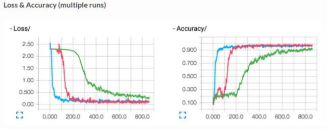
Figure 19 Tensorboard training process visualization example. (53) ... 31

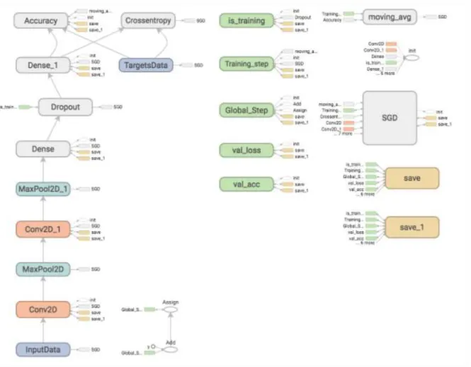
Figure 20 Tensorboard network visualization example. (53) ... 32

Figure 21 MNIST dataset ... 35

Figure 22 CIFAR-10 dataset ... 36

Figure 23 2-D representation of the Euclidian distance ... 39

Figure 24 Visual representation of the K-Nearest Neighbours algorithm on a 2-D plane (59) ... 41

Figure 25 Representation of different classification outcomes based on the value of K. (60) ... 42

Figure 26 Visual representation of a three layer multilayer perceptron (26) ... 43

Figure 27 Multilayer Perceptron Architectures: From the left: MLP-3, MLP-4, MLP-5 ... 46

Figure 28 Simple convolutional neural network ... 47

Figure 29 VGG ... 48

Figure 30 Residual learning block (67) ... 49

Figure 31 Residual Convolutional Block ... 50

Figure 32 ResNet-18 ... 51

Figure 33 Block Inception-A. (69) ... 52

Figure 34 Block Inception-B. (69) ... 52

Figure 35 Block Inception-C. (69) ... 52

Figure 36 Prime Inception ... 53

Figure 37 Visual representation of layer concatenation. ... 54

Figure 38 Visual representation of layer element-wise summation. ... 54

Figure 39 SaraNet-P ... 55

Figure 41 Visual presentation of dropout. On the left: neural network without dropout. On the

right: neural network with applied dropout. ... 59

List of tables

Table 2 Mobile Computation Unit ... 34

Table 3 Accuracy results ... 62

Table 4 Speed benchmark... 63

Content

LIST OF FIGURES ____________________________________________ 6

LIST OF TABLES _____________________________________________ 7

1.

INTRODUCTION _________________________________________ 10

1.4.4. ImageNet – Large Scale Visual Recognition Challenge ... 17

1.5. Contributions ... 18

1.6. Structure of the Work ... 18

2.

DATA __________________________________________________ 19

2.1.1. COMSOL Multiphysics as data acquisition environment ... 21

2.1.2. Details of the simulation ... 26

2.1.3. Objects of the experiment ... 27

2.1.4. Deep Learning Libraries ... 30

2.2. Benchmark ... 33

2.2.1. Hardware and Software Specification ... 33

2.2.2. MNIST ... 35

2.2.3. CIFAR-10 ... 36

3.

METHODOLOGY ________________________________________ 37

3.1.1. Label encoding ... 37

3.2. k-Nearest Neighbours ... 38

3.3. Multilayer Perceptron Network ... 43

3.4. Convolutional Neural Networks ... 46

3.4.1. Simple convolutional neural network ... 46

3.4.2. VGG-16 ... 47

3.4.4. Prime Inception ... 51 3.4.5. Stacked Artificial Residual Architecture (SARA-Net) ... 55

4.

OPTIMIZATION __________________________________________ 58

5.

RESULTS ______________________________________________ 62

6.

FINANCIAL ANALYSIS ____________________________________ 65

7.

FINAL THOUGHTS _______________________________________ 66

8.

APPENDIX A – CODE _____________________________________ 68

9.

BIBLIOGRAPHY _________________________________________ 69

1. Introduction

1.1. Background

Machine learning is a field of data science that is utilized in every aspect of our lives. From entertainment with Netflix (4), through shopping and personal assistants with Amazon (5) and Google (6), to automatized medical recommendation with Deep Mind (7) and fraud detection with Paypal (8). Certainly these services changed how we perceive the world. A comparison can be drawn between the current development of the artificial intelligence industry and the Automation Revolution. During the Automation Revolution many tasks have been improved by introducing robots. They were cheaper, faster and could work 24 hours a day, 7 days a week, unlike humans. However, they were limited to simple and repeatable tasks. Complicated tasks that required creativity or imagination were out of the reach.

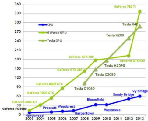
Utilization of Artificial Intelligence was still a dream, even with proofs of concept laid out by scientists, like Frank Rosenblatt (9) and Stephen Grossberg (10). The technological limitations were too big. The biggest of them was limited computational power available to the industry. Even giants, like IBM, did not have resources powerful enough in order to make machine learning their core business. That changed in recent years with development of Graphic Processing Units (GPUs). GPU contains of thousands of cores, which are capable of running parallel calculations (11). It enables the hardware to calculate physics, lighting and game engine logic in an extremely fast manner. That happens with multiplication of an huge number of variables in fractions of a second.

to growth of processing power of Central Processing Units (CPUs):

Figure 1 Comparison of GPU and CPU data processing capabilities (12).

High speed, cheap computational capability is the core of the artificial intelligence revolution by providing affordable, financially and time-wise, solutions.

The biggest GPU manufactures in the world, Nvidia, introduced parallel computing

platform CUDA (13) and deep neural network primitives cuDNN (14), which resulted in even higher speed calculations. Finally, that sums up to 20 times speed increase comparing to Computational Processing Units (CPUs) (15).

Finally, deep learning by its nature is capable of assigning weights to all the input parameters. That result in process similar principal component analysis, where importance

of any feature is assessed. That approach is appealing to both business and engineers by reducing the required effort. Along with cheap, powerful computational power and ease to use, deep learning has become a go to solution.

1.2. Problem

Problem of object shape detection based on the magnetic field disturbance was introduced in Spring 2016 by ABB Corporate Research to students of InnoEnergy’s Smart Electrical Networks and Systems Double Degree Programme. As part of the Industrial Innovation Project course, author of this thesis along other students was challenged to build a autonomously flying drone with a magnetic field measurement system attached to it. The goal of the project was to build a minimum viable product, which could scan a certain area with minimum supervision. The project was planned to be later on improved to a swarm of drones, which could avoid obstacles and decrease the scanning time.

The project proved to be challenging. After a discussion between the industrial supervisors, Ara Bissal and Salinas from ABB, and the students, a decision was made to divide the project into two part: autonomously flying drone and data analytics of the scan. It is of a big interest to create such system in order to assess features of the detected object such as shape, size and possible danger it poses, especially in a remote location.

Furthermore, this project combines two biggest automation trends: utilization drones and artificial intelligence. Following self-flying drones inspecting wind turbines (16), delivering goods (17) (18) or saving lives (19) (20), this thesis tests if self-flying drones with magnetic field disturbance detection can successfully classify shape of an object.

1.3. Limitations

This thesis tackles a very specific problem. It was necessary to narrow it down in order to perform the experiment according to the standards. It should be treated as an initial stage of a technology test and possibly product idea prototype.

Firstly, set of possible shapes is infinite. In this thesis, 4 very specific shapes were chosen as the test subjects. Computationally heavy calculations , like physics simulation and neural network training, were the biggest obstacle in terms of available resources. Thus, this thesis should be treated as a proof of concept.

Secondly, drone location and altitude accuracy has a tremendous impact on the data. This issue is detrimental to the success of the project especially with external environmental disturbances (f.e. wind) or natural and artificial obstacles (f.e. trees, buildings or remote location) as a big factor. Author of this thesis focuses on building system that would successfully differentiate between different shapes and the drone hardware limitations are outside of the scope of the project, thus the drone is assumed to be ideal.

Finally, machine learning is an extremely big and tremendously fast developing field. Set of algorithms presented in this thesis is specifically chosen to the nature of the data, which is presented as a two dimensional image. That approach was chosen in support with experience and knowledge of the author of the thesis, and confirmed by the practises from the research community.

1.4. Related work

1.4.1. Similar work

Magnetic field is not the most common source of information in machine learning. In most cases sound- or light-based systems dominate as they provide extensive and easy to interpret amount of data. Magnetic field-based system have been used mostly for indoor localization (21) (22) and earthquake prediction (23). On top of that, few research experiments have been performed utilizing magnetic field for iron prospectivity (24), gold field structural exploration with aeromagnetic data (25) and prediction of the concentration of the iron ore (26) .

Despite that these research projects approached the visualization of the data in the same way as presented in this thesis, none of them utilized the most advanced image recognition algorithm – convolutional neural networks.

1.4.2. Neural Networks

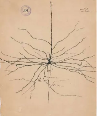
In 1889, Spanish neuroscientist Santiago Ramon y Cajal presented a model of a neuron and the nervous system. Despite a strong critique and opposition, his work resulted in paper

Textura del Sistema Nervioso del Hombre y los Vertebrados, which started a new branch of science – neurology (27). For that achievement he was rewarded the Nobel Prize in 1906.

Figure 2 Pyramidal neuron of the cerebral cortex by Santiago Ramon y Cajal (28)

The idea was further developed byWarren McCulloch, Walter Pitts (29) and later by Frank Rosenblatt (30) resulting in a binary computational model of a neuron called Perceptron. However, one layer of perceptrons was capable of solving only linear problems (31), which is a major limitation. In 1960’s this problem was solved with introduction of nonlinear activation functions (32).

1.4.3. Image recognition

Earliest computer vision concepts are dated in 1960’s. At this time Larry Roberts, a PhD student from MIT, introduced so called low level tasks as a necessity to obtain initial understanding of the object. These tasks included edge detection, segmentation etc. They were constructed by a very qualified engineers, however they were limited by human understanding of the surroundings. This approach was applied by David Marr in 1978 and

was a major breakthrough (33). However, with time, this approach was proven not scalable and inefficient.

In 1989 Yann Lecun published a ground-breaking paper (34) introducing convolutional neural networks.

Convolutional neural network is a subset of neural network that is specialized in learning data that can be presented in a grid (35). That applies to image recognition, where the data can be presented as two-dimensional tiles and in natural language processing, where the sequence is mapped into as one-dimensional.

Concept of convolutional neural networks can be compared to applying filters on a picture. With a filter or group of filters the picture can reveal valuable information, enhance certain shapes or show horizontal or vertical edges. In 90’s automatic image recognition was still performed with specially engineered features (36).That approach was inefficient and led to huge overhead, since man-made filters was based on human perception. It would be doubtful to try to solve problems the natural language processing in the same manner.

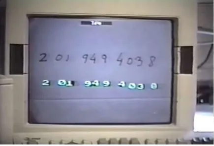
Convolutional neural network proved to be efficient in learning hand-written digits with artificially learned features.This approach achieved over 99% accuracy (37). The experiment was re-created by the author of this thesis and results can be found in chapter 5. Results.

Figure 3 Handwritten digit recognition with a back-propagation network. (38)

1.4.4. ImageNet – Large Scale Visual Recognition Challenge

ImageNet is a large scale visual recognition challenge. It is hosted annually since 2010 (39). It was inspired by Pascal VOC challenge, started in 2005. ImageNet provides a publicly available dataset and competition workshop. Participants of the challenge train their models with a special training set of images, manually annotated by the hosts of ImageNet. Predicted labels obtained by the participants are submitted to the evaluation server. After each period, results on the testing data are revealed and the conclusions and research are shared at the International Conference on Computer Vision (ICCV) or European Conference on Computer Vision (ECCV).

ImageNet challenges can be divided into two part: image classification and object detection. The image classification challenge focuses on answering the question is there object X on this picture or not. On the other hand, object detection challenge focus on detecting and marking an object in the image, f.e. by drawing a rectangle around it.

ImageNet provides an extremely valuable data. In 2017, the training dataset consists of 1.2 million images presenting 1000 labels. During existence of the competition, image recognition has improved to superhuman level (40) (41).

1.5. Contributions

This thesis presents a vast amount of machine learning algorithms (kNN, MLP and CNN) and architectures in context of physical data gathered by a drone. The author of the thesis re-created the most known and advanced computer vision architectures (VGG and ResNet) and proposed two additional architectures inspired by the research.

1.6. Structure of the Work

Chapter 1 : Introduces the problem, limitations and related work.

Chapter 2 : Describes the simulation environment and how the data was obtained and pre-processed.

Chapter 3 : Discussed the methodology, architectures of the networks including building blocks.

Chapter 4 : Explains optimization techniques used to obtain the best results.

2. Data

2.1. Processing Pipeline

Machine learning experiment is a process that can be divided into a few, major steps. According to Jean-François Puget from IBM (42) machine learning workflow is as follows:  Data acquisition

 Data preparation

 Choosing the best model

 Creation of the model

 Deployment

 Prediction

 Monitoring and Improvements

Data acquisition is a fundamental step in every machine learning experiment. In the context of machine learning, information is the most important asset, since machine learning optimization is a data-based process.

Acquisition of the data required for the success of the thesis is very difficult. Assuming a successful implementation of the previously mentioned autonomous drone measurement system, the amount of data and external factors, (like weather or hardware difficulties) and required resources, like knowledge and time of very skilled employees, could be not profitable.

measurement process by simulating it with a multi-physics software. The process is described in details in chapter 2.1.1. COMSOL Multiphysics as data acquisition environment.

After a successful simulation the data needs to be pre-processed. The data is presented as a 2-D grey scale picture, instead of more appealing for human eye 3-D colour picture . This approach puts emphasis on the complexity of the networks by diminishing the input dimensionality while carrying the same information (43). Furthermore, the information is encoded as in numbers in range (0, 255), which is very problematic for neural networks since it causes saturation and dead ReLu issues (44). In order to avoid these issue, the data is normalized with MinMax technique as follows (45):

(1) 𝑋 = 𝑋 − 𝑋

𝑋 − 𝑋

Where:

 𝑋 - normalized dataset (in range from 0 to 1)  𝑋 - original dataset (in range from 0 to 255)  𝑋 - minimal value of X

 𝑋 - max value of X

The data is stored as a 3-D array that can resemble a sequence of frames and further accessed while training the neural networks.

The data is divided into subset for cross validation. Process of cross validation is presented in chapter 4.1 Cross-validation. At this point, data pre-processing is finished.

recognition is a huge part of machine learning, however each problem backed by a specific dataset should have adjusted architecture. State-of-the-art architectures are generally good in most of the situations, however they require a huge computational power. Thus, unwise is use of previously mentioned algorithms without any knowledge about the complexity of the problem. It can results in a pessimal utilization of resources.

Thus, this thesis focuses on both simple algorithms (chapter 3.2. k-Nearest Neighbours) and (chapter 3.3. Multilayer Perceptron Network and chapter 3.4.1. Simple convolutional neural network, state-of-the-art approaches (chapter 3.4.2. VGG-16 and chapter 3.4.3. ResNet-18) and introduces two additional architectures inspired by the resent development in the field (chapter 3.4.4. Prime Inception and 3.4.5. Stacked Artificial Residual Architecture (SARA-Net)).

Following, the algorithms are implemented in Python 3.5 with libraries Tensorflow and TFLearn. Argumentation behind the choice is presented in in chapter 2.1.4. Deep Learning Libraries. The implemented algorithms are deployed on a local personal computer with a graphic processing unit. Prediction is performed on a laptop in order to test the mobility of the solution. The specifications is presented in chapter 2.2.1. Hardware and Software Specification.

Various variables of the networks are optimize during the training process with help of validation dataset. Optimization methods are described in chapter 4. Optimization.

2.1.1. COMSOL Multiphysics as data acquisition environment

COMSOL is a multi-physics simulation software created by The COMSOL Group (46). It enables a simulation of various physical scenarios, including high and low frequency

electromagnetics, fluid dynamics, chemical reactions and many more. The biggest strengths of COMSOL regarding this thesis are:

- Simple workflow

- Parametric Sweep

- Rich information export options COMSOL’s workflow is as follows (47):

Firstly, the user chooses physics modules, study mode (stationary, dynamic or frequency analysis) and the dimensionality of the problem.

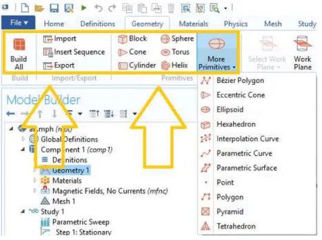
Secondly, the objects of the simulation are created. Since the native object creation tools are limited, COMSOL enables import of figures and shapes from CAD software.

Figure 4 Process of adding new geometry in COMSOL Multiphysics

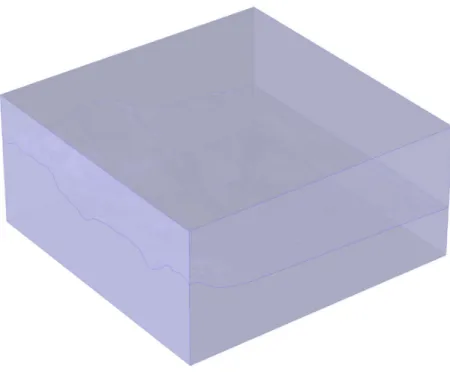
software has a rich build-in library, however adding custom material is possible as well. Next step contains physics setup. It is important to mention that every simulation requires boundary condition. A box of size encapsulating the environment simulates the boundary conditions:

Figure 5 Boundary condition setup in COMSOL.

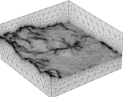
In order to perform the simulation, the geometries are approximated by a mesh. Custom mesh is chosen in order to perform a very accurate simulation.

All surfaces (the Earth surface, the object and the boundary condition surface) are covered by an extremely fine mesh:

Figure 6 Earth surface mesh approximation

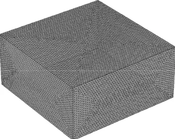
Figure 8 Boundary conditions surface mesh approximation

COMSOL enables experiment with parametric sweep. In this context, parametric sweep is a series of simulation with different values of parameters. Orientation of the object will be changed in order to simulate different position in comparison to the magnetic field.

Objects of the experiment are localised in one specific point under the ground. The reference point is the centre of the object (for the cube) or in the centre of the base (for the rest of the shapes) which has fixed coordinates. The object is rotated counter clockwise (angle phi Φ from 0 to 330 degrees every 30 degrees) and (tipping angle theta ϴ from 0 to 90 degrees every 15 degrees). That approach results in data corresponds to a 84 possible locations in a remote location and creates more samples for the network.

Finally, the data is exported. The measurements are presented as a set of 2D grey scaled one layer pictures. From practical point of view, it is impossible to perfectly assess if where is the centre of the After further down sampling of the results, each image outputs 121 image.

2.1.2. Details of the simulation

The simulation was performed based on Magnetic Prospecting of Ore Deposits example provided by COMSOL (49). Area of the simulation is surrounding of Eagle Mountain Mine, place of former Kaiser Steel Co. mining operation in Riverside County in California, USA localized N 33.85°, W 115.5° (50).

The Earth magnetic field is simulated by a constant uniform magnetic field given as:

(2) ∇( −μ ∇V + B ) = 0

Where:

 𝐵 is the (background) geomagnetic flux density,  𝐵 is the remanent flux density

 𝜇 is the magnetic permeability of the material  V is the magnetic potential

Geomagnetic information is obtained from The National Centre of Environmental Information (50):

𝐵 = 48.163𝜇𝑇

𝐼𝑛𝑐𝑙𝑖𝑛𝑎𝑡𝑖𝑜𝑛 = 59.357° 𝐷𝑒𝑐𝑙𝑖𝑛𝑎𝑡𝑖𝑜𝑛 = 12.275°

Material properties were adjusted to simulate properties of iron ore as a homogeneous magnetite ore as suggested in (50).

2.1.3. Objects of the experiment

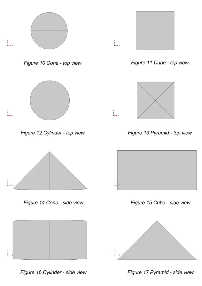
Objects simulated for this thesis are 4 basic shapes: cone, pyramid, cylinder and cube .These objects are specifically chosen to resemble each other and make the classification task relatively difficult. At the same time, number of the shapes was limited due to limited computational power. The objects are placed just under the surface of the ground (approximately 0.5 meter depending on the measurement reference). Material of choice is iron, since it is disturbs the magnetic field on a significant level and is a common material at the same time.

Figure 10 Cone - top view Figure 11 Cube - top view

Figure 12 Cylinder - top view Figure 13 Pyramid - top view

Figure 14 Cone - side view Figure 15 Cube - side view

They are defined in the simulation environment as follows:  Cone o Bottom radius = 5 m o Height = 10 m o Top radius = 0.5 m  Pyramid

o Base length 1 = 10 m (corresponding to x-axis) o Base length 2 = 10 m (corresponding to y-axis) o Height = 10 m

o Ratio = 0.01

o Top displacement 1 = 0 m (corresponding to x-axis) o Top displacement 2 = 0 m (corresponding to y-axis)

 Cylinder o Radius = 5 m o Height = 10 m  Cube o Width = 10 m o Depth = 10 m o Height = 10 m

2.1.4. Deep Learning Libraries

Deep learning is a heavy computational process. That requires specialized software in order to perform the computation in the most optimized way. This thesis utilizes two highly sophisticated libraries: Tensorflow and TFlearn.

Quoting (51):

TensorFlow™ is an open source software library for numerical computation using data flow graphs. (…)TensorFlow was originally developed by researchers and engineers working on the Google Brain Team within Google's Machine Intelligence research organization for the purposes of conducting machine learning and deep neural networks research, but the system is general enough to be applicable in a wide variety of other domains as well.

Tensorflow has few tremendous advantages.

Firstly, it is optimized to perform computations on multiple GPUs, both locally and on a remote distributed systems. This feature alone can speed up training time 10-20 times (52).

Figure 18 GPU vs CPU training. (52)

popularity (source) in recent years due to its readability and simplicity. Furthermore, back-end of Tensorflow is written in C / C++. That results in high speed, which has always been the biggest argument against using Python in data science.

Next, Tensorflow has an integrated visualisation tool – Tensorboard. Tensorboard can show all vital variables for each training step, like training and validation accuracy, value of the loss function and visualize the architecture of the network. These two components have a tremendous impact on the process of optimization of the parameters of the network.

Figure 20 Tensorboard network visualization example. (53)

Finally, Tensorflow is a low-level library. That gives a huge freedom in terms of creation of new architectures and algorithms. However, it makes the creation of networks based on already known and deeply studied building block a time consuming task.

For that reason, another deep learning library was introduced – TFLearn. TFLearn is a high level wrapper around Tensorflow. It was created by Aymeric Damien, former research assistant at Tsinghua University and current Software Engineer at Snapchat. It packs vital machine learning blocks, like convolutional layer, fully connected layer and cost functions into few lines of code (53). With that, the code is much more modular, easier to read and less

susceptible to bugs. That comes with price of customization, however, it was not an obstacle for system presented in this thesis.

2.2. Benchmark

2.2.1. Hardware and Software Specification

Specifications of the local and mobile computation units are presented in tables below:

Table 1 Local Computation Unit Specification

Processor Intel® Core ™ i3-3225 @ 3.30 GHz x 4

RAM 8GB

Graphic Processing Unit Nvidia GeForce GTX 970

Operating System Ubuntu Linux 16.04 64-bit

Hard Disk KINGSTON SV300S37A120G

Tensorflow version 1.1.0, GPU enabled

TFLearn version 0.3.2

GPU drivers Nvidia 375.66

CUDA version 8.0

Table 2 Mobile Computation Unit

Processor Intel® Core ™ i5-3317U @ 1.70 GHz x 4

RAM 8GB

Graphic Processing Unit Nvidia GeForce GT 740M

Operating System Ubuntu Linux 16.04 64-bit

Hard Disk TOSHIBA MQ01ABD075

Tensorflow version 1.1.0, CPU only

TFLearn version 0.3.2

GPU drivers X.org Noveau

CUDA version Not Applicable

2.2.2. MNIST

Benchmark of the networks was performed on two most common supervised machine learning datasets: MNIST and CIFAR-10.

MNIST dataset is a large dataset of handwritten digits. It contains of 70 000 examples from approximately 250 writers (54) in grey scale. The size of the images (28 by 28 pixels) enables test on very large networks, however classification of the correct labels with accuracy above 99% has been proven constantly achievable even with simple network architectures.

The dataset has been cited multiple times by the most respected researches like Yann LeCun, Yoshua Bengio and Juergen Schmidhuber (37) (54) (55).

2.2.3. CIFAR-10

CIFAR-10 is another very popular image recognition dataset. It was collected and pre-processed by scientist from Massachusetts Institute of Technology (MIT) and New York University (NYU) (56). It contains of 60000 examples of images of size 32 by 32 pixel with 3 channels, which represent red, blue and green colours. The data presents 10 objects: airplane, automobile, bird, cat, deer, dog, frog, horse, ship and truck. It has been more challenging than MNIST (56), however usually a various additional pre-processing methods have been implemented in order to achieve high accuracy. These methods are outside of the scope of this thesis.

3. Methodology

3.1. Supervised Machine Learning

Supervised machine learning is a branch of machine learning focused on finding relations between known inputs and outputs. This relation can be expressed in two different ways, based on the nature of the problem: regression and classification. Regression is a relation between input and output, when the output is continuous. This approach is often use in sequence prediction of stock prices or weather variables, like temperature and atmospheric pressure. On the other hand, classification system returns labels. Thus, the problem is discretized.

3.1.1. Label encoding

Often made mistake is that the labels are encoded as f.e. 1, 2, 3, 4… This approach is wrong, which can be explains in an example:

Assuming the system has three labels, encoded as 1 ,2 and 3, which correspond to three states of the output. After successful training of the training data and confirmation from the validation data, we ensure that the system is relatively accurate and can successfully generalize. During production test, the system outputs value 2. Taking into consideration all the possible scenarios, we are unable to assess if the system is perfectly sure that the correct class or we are completely unsure (50% - 50%) that the output should be either class 1 or class 3.

labels into an array of probabilities. Usually, train, validation and test labels are known so the correct label can be encoded with probability of 1. With that:

 Label 1 is encoded as [100]  Label 2 is encoded as [010]  Label 3 is encoded as [001]

This approach results in a very clear outcome. If the system is sure that the correct label is 2, the output will be [010], however if the system is completely unsure (50% - 50%) if the correct label is 1 or 3, the output will be [0.500.5].

3.2. k-Nearest Neighbours

K-Nearest Neighbours is one of the most simple supervised machine learning methods. It is a so called non-parametric or lazy algorithm. Non-parametric methods are methods, which do not learn any parameters. They rather access previous stored data and compare the new input and output a value, in case of regression, or a class, in case of classification.

K-Nearest Neighbours algorithm can be summarized in few step: 1) Receive a new input

2) Access the stored data, which contains of both inputs and outputs of the system 3) Compare the new input and the input from the stored data

5) Return the output

As presented above the kNN algorithm can be compared to a database. It accesses the stored data and based on the observation, returns an output.

The output can be calculated in based on the Mahalanobis distance or energy based classification, and Euclidian distance. This thesis will focus only on the last approach. Euclidian distance 𝑑 (57) is a 𝑅 metric given as:

𝑑 = ‖𝑥 − 𝑦‖ = (𝑥 − 𝑦 ) + (𝑥 − 𝑦 ) + ⋯ + (𝑥 − 𝑦 ) (3)

The Euclidian distance represented in a two dimensional space is presented below:

Figure 23 2-D representation of the Euclidian distance

It is crucial to fully understand the algorithms and its limitation. The algorithm calculates distances between the new input and all the labelled data points. Next, the

distances are compared and points with the lowest Euclidian distance to the input are of the biggest value.

Let’s assume a 2-D situation with 𝑁 data points, which belong to class 𝐶 and number of all points is denoted as 𝑁. In order to classify the class of the new object, we draw a circle with centre in the new point. This circle contains of 𝐾 labelled points and has an area A. There are 𝐾 points of class 𝐶 .

With that the density for each class is given as:

(4) 𝑝(𝑥|𝐶 ) = 𝐾

𝑁 𝐴

Density for all the whole dataset is given as:

(5) 𝑝(𝑥) = 𝐾

𝑁𝐴

Furthermore, probability of class 𝐶 in the whole dataset is given as:

(6) 𝑝(𝐶 ) =𝑁

𝑁

Using Bayes’ theorem (58), the probability of point 𝑥 belonging to class 𝐶 is given as:

(7) 𝑝(𝐶 |𝑥 =𝑝(𝑥|𝐶 )𝑝(𝐶 )

𝑝(𝑥) =

𝐾 𝐾

Thus, the probability of that the point 𝑥 belongs to a class 𝐶 is proportional to number of points 𝐾 that belong to class 𝐶 and are inside a circle of area 𝐴 divided number of all

name K-Nearest Neighbours. The circle is drawn in a way that it contains all 𝐾 closest points and the label of the new point is based on the representation of the class in the circle. Visual representation of the process it shown below:

Figure 24 Visual representation of the K-Nearest Neighbours algorithm on a 2-D plane (59)

This approach has few advantages.

Firstly, it is a very simple algorithm. Implementation of the algorithm with current advanced libraries like Scikit-learn is extremely fast and simple.

Secondly, the algorithm does not require pre-training. Since the behaviour of the K-Nearest Neighbours algorithm is similar to a database, the relation between the input and the output is learned in real time.

Figure 25 Representation of different classification outcomes based on the value of K. (60)

Finally, the optimization of the algorithm is a straightforward process. Predictions for the validation dataset are made based on the training dataset for a range of values of parameter 𝐾 and the evaluated with the validation dataset. The chosen variable 𝐾 is the one that produces the highest accuracy for the validation dataset.

However, it is important to mention disadvantages of the K-Nearest Neighbours algorithm.

Firstly, it strongly depends on the local distribution. KNN is a lazy algorithm, which does not learn any relations between the input and the output. Thus, it is extremely susceptive to misclassification in areas poorly covered by the training dataset.

Secondly, it scales very poorly. The prediction time grows linearly with number of the training samples and with the number of features.

Finally, the biggest issue is that it requires a continuous access to the data. Taking into industrial application of the technology developed in this thesis, an undisturbed access to the data is a tremendous issue. In some cases it might exclude the algorithm as

impractical.

Results of the benchmark for the algorithm are presented in chapter 5. Results.

3.3. Multilayer Perceptron Network

Multilayer Perceptron is an artificial neural network that consists of multiple layers of perceptrons (61). The perceptrons are activated by nonlinear functions in order to enable the network to learn nonlinear relations between the input and the output.

Figure 26 Visual representation of a three layer multilayer perceptron (26)

Output of the first hidden layer is given as:

Output of the second hidden layer is given as:

(9) ℎ = (𝑤 ℎ + 𝑏 )

General rule of the data flow can be drawn:

(10) {𝑙|𝑙 ∈ 𝐿}, 𝑂 = (𝑤 𝑂 + 𝑏 )

Where:

 𝑂 is output of the layer  𝑙 is index of the layer

 𝐿 are all layers except the input layer

The prediction is calculated based on the same principle:

(11) 𝑦^ = (𝑤 𝑂 + 𝑏 )

Difference between the prediction and the correct label is called loss function. The loss function depends on the nature of the problem.

For a regression the most common loss function is MSE (Mean Squared Error) given as:

(12) 𝑀𝑆𝐸 =1

For a categorical problem, when the object can belong only to one category, the most common cost function is categorical cross entropy (62):

𝐻(𝑦, 𝑦^) = − 𝑦 𝑙𝑜𝑔(𝑦^) ₍₁₃₎

Where:

 𝑦 is the correct label (encoded as 1)

 𝑦^is the predicted probability that the object belongs to the class

The cross entropy is a logistic likelihood that the prediction is correct. It is crucial to mention that the logistic likelihood is a much stronger metric than accuracy, because it puts emphasis on the confidence of the prediction.

In this thesis, 3-, 4- and 5-layers architectures has been tested. In each architecture dropout was applied only on last two fully connected hidden layers in order unify the approach and achieve highest accuracy.

Figure 27 Multilayer Perceptron Architectures: From the left: MLP-3, MLP-4, MLP-5

All three architectures were tested with two different setups: with 1000 neurons in each fully connected layer.

The results are presented in chapter 5. Results.

3.4. Convolutional Neural Networks

3.4.1. Simple convolutional neural network

The first convolutional neural network architecture proposed in this thesis is a simple, two layer convolutional neural network. It consists of two convolutional layers with kernel 2 by 2 stacked on each other and two fully connected layers with dropout (details in chapter 4.2. Dropout).

All layers are activated by a rectified linear unit (ReLu).

Figure 28 Simple convolutional neural network

(63) suggests that stacking two convolutional layers with small filters results in higher level of abstraction than with one convolutional layer with big filter. Furthermore, as proven in (63) large filters are computationally inefficient. Thus, this simple architecture was designed with focus on simplicity and computational efficiency.

The network was tested with different number of filters and the results are presented in chapter 5. Results.

3.4.2. VGG-16

VGG-16 is an architecture introduced by Visual Geometry Group from Oxford (64). During ImageNet ILSVRC-2014, the network achieved first place in the localization task and second in the classification task (65). These tasks are described in details in (39).

VGG-16 consists of multiple convolutional layers stacked upon each other. Filters 3 by 3 were chosen, which has been proved more efficient that bigger filters (63). A very

distinguish feature of this network is that it has an extensive number of filters in each layer, ranging from 64 to 512, that doubles every block. Max pooling with kernel 2 by 2 follows each block in order to effectively shrink the size of the image by 4. That operation results in a loss of data, but it is necessary in order to reduce the dimensionality of the picture, thus reduce the calculation time. All layers are activated by a rectified linear function, which does not suffer from saturation. Convolutional layers are followed by two fully connected layers.

According to (64), the network consists of 144 million parameters. The architecture was trained with minibatch gradient descent with momentum (64), however the author of the thesis decided to train the network with Adam optimizer (66) in order to perform full comparison between the networks based only on their structures. Results are presented in chapter 5. Results.

3.4.3. ResNet-18

ResNet is a deep residual architecture introduced Kaiming He, Xiangyu Zhang, Shaoqing Ren and Jian Sun from Microsoft Research in paper (67). In recent years improvement of the image recognition task was achieved by stacking a tremendous number of layers on top of each other (64), thus the authors of the paper question that approach and introduced Residual Block.

A residual block is a block consisting of two weight neural network layers and an identity mapping:

The result of the transformation is given as:

(14) 𝐻(𝑥) = 𝐹(𝑥) + 𝑥

In case of a two dimensional image recognition, weight layer is substituted by a two dimensional convolutional neural network.

Figure 31 Residual Convolutional Block

Result of the operation can be interpreted as enhancing the found features on the original picture.

Batch normalization is applied after each convolution layer and before the activation function as suggested in (67).

Finally global average pooling is utilized on the last convolution and a fully connected layer with softmax activation function returns the probability of each of the classes.

validation error (67), shallower 18-layer architecture was chosen:

Figure 32 ResNet-18

Performance of the network is presented in chapter 5. Results.

3.4.4. Prime Inception

Deep Prime Inception is the first novel architecture introduced in this thesis. The architecture was inspired by research performed by GoogLeNet team from Google and Zbigniew Wojna from University College London (68).

At the turn of 2015 and 2016 they introduced few building blocks of an Inception V4 network (69):

Figure 33 Block Inception-A. (69)

Figure 34 Block Inception-B. (69)

The novelty of this approach is that it combines parallelly connected branches of stacked convolutional neural layers. Thus, certain layers are capable of learning feature independently of other branches. Based on that, author of the thesis introduces Prime Inception Network:

Figure 36 Prime Inception

Prime Inception network is an architecture that combines few different concepts: Firstly, concept of convolutional neural networks stacked in order to achieved high level of abstraction. Different sizes of the features are implemented in order to provide different range of view for the network.

Secondly, in principle, with 4 independent branches the network should be capable of learning and combining different levels of abstraction.

Finally, the branches are merged together. Two versions of the merging procedure produce two versions of the network: Prime Inception - C and Prime Inception – ES. Prime Inception – C concatenates all the filtered images together resulting in number of filters equal to 4 times of filter of each branch. Prime Inception – ES merged the adds the filters element-wise resulting in number of filters each to number of filters in each branch.

The process is presented below:

Figure 37 Visual representation of layer concatenation.

3.4.5. Stacked Artificial Residual Architecture (SARA-Net)

Stacked Artificial Residual Architecture is the second novel architecture presented in the thesis. It is built upon idea of ResNet, where outputs of certain convolutional layers were used further as identity connections. Novelty of the Stacked Artificial Residual Architecture is that all outputs of the convolutional layers are reused as inputs to next convolutional layers. Two different filter kernel configurations are investigated: Prime Configuration and 3x3 Configuration. Prime configurations (denoted as SaraNet-P) contains of kernel sizes of consecutive convolutional layers equals to 7x7, 5x5, 3x3 and 2x2 as presented below:

3x3 configurations (denoted as SaraNet-3x3) utilizes much smaller and more computationally efficient filters of size 3 by 3.

The network is presented below.

Figure 40 SaraNet-3x3

The data is merged by either concatenation (denoted with suffix -C) or element-wise sum (denoted with suffix -ES). That results in 4 networks:

 SaraNet-P-ES

 SaraNet-3x3-ES

 SaraNet-3x3-C

Due to high number of parameters, last merging layers of SaraNet-P-C and SaraNet-3x3-C are down sampled with maximum pooling operation.

4. Optimization

4.1. Cross-validation

Cross-validation is a hyperparameter optimization technique. Hyperparameters are parameters that are not learned during the training of the network. They need to be set by an experienced engineer after a set of experiments involving a specific dataset. A simple cross-validation process results in a split of the dataset into three subsets: training dataset, validation dataset and test dataset. This approach is important as information to the network can be provided both directly and indirectly (70). A neural network adapts its weights based on the training dataset, which is a direct flow of information. The network has access to every piece of information provided to it, both as inputs and outputs. As explained in chapter 4.2. Dropout prediction over the training dataset cannot be trusted due to risk of overfitting. Thus, the best model will be chosen based on performance over the validation dataset. That provides an indirect flow of information. Combining direct flow of information provided by the training dataset and indirect flow of information by performance metrics over the validation dataset and choice of the hyperparameters based on that, the network is pushed to its boundaries of a successful generalization.

In this thesis, the whole dataset will be split into the training set and dataset with proportion 90% to 10%. Then the training set is divided into a new training set and a validation training set in proportion 80% to 20% as suggested in (35).

4.2. Dropout

Dropout is an optimization technique that engages in the internal structure of the network. By applying dropout certain connections between the neurons are omitted with certain probability. Each epoch all connections are restored and new set of connections are dropped.

Figure 41 Visual presentation of dropout. On the left: neural network without dropout. On the right: neural network with applied dropout.

Dropout counteracts overfitting, where the network does not learn how to successfully generalize, but it simple remembers the data and tries to mimic it as best as possible (71). Data provided to any network is just a subgroup of all data that could be gathered in order to present a phenomenon. Thus, remembering a subset of data is not a sufficient proof of being able to successfully generalize.

Additional issue that occurs with large neural networks is the hyperparameter optimization. Dropout results in exponential increase of the network configuration within one

architecture (71). That approach can be compared to the Random Forest Algorithm (72). Aftereffect of random recombination of connections inside the network arise as a more robust and steady architecture. Dropout of 50% can be understood as that all the possible network recombination are equally important. Interchanging them each iteration with weight sharing is a very efficient way of prediction using multiple connection model. As presented in (73), dropout of 50% increases the accuracy of the prediction by even 3-5%.

4.3. Best model re-load

Training a neural network is a very complex process. During that time, millions of parameters are adjusted for the best performance. It introduces a number of possible phenomenon that could lead to performance far from the capabilities of the architecture. One of them is overfitting. Overfitting occurs when the network adjust so much to the training data that it can be said that it remembers the data. Typically it can be seen when the loss function calculated over the validation dataset rises with number of analysed samples. That results in accuracy lower than optimal.

In order to counteract this issue, author of this thesis used best model re-load feature provided by TFLearn. After each epoch the network is evaluated in terms of performance over the validation dataset. The measure of the performance is the categorical cross-entropy, which has been introduced in chapter 3.3. Multilayer Perceptron Network. This specific measure was chosen over the accuracy metrics due to fact how both of them are calculated during the training.

Let’s analyse an example:

During an epoch of the training, few samples were correctly assigned with certain probabilities. The very next epoch, same samples were again correctly assigned but with higher probabilities. Since there is no change in the accuracy over the samples (in both cases it is equal to 1 over the samples), the system would not save the training checkpoint as the best despite the fact the network is much more confident in its prediction. For the same case, categorical cross-entropy would present a difference since its operates on the probabilities. The smaller the loss function, the closer the prediction to the real values.

Author of this thesis decided to train all the networks for 100 epochs, during which the best model is saved. Next, the best model is re-loaded to provide the best performance and the final evaluation is performed.

5. Results

5.1. Accuracy

Table 3 Accuracy results

Network \ Data MNIST CIFAR-10 Shape classification based on the

magnetic field disturbance

kNN 97.00 Out Of Memory Out Of Memory

MLP-3 98.51 55.14 98.08 MLP-4 98.53 53.22 98.30 MLP-5 98.29 52.06 98.50 Simple CNN 99.01 61.49 98.99 VGG - 16 99.29 78.76 100 ResNet - 18 99.25 67.18 100 Prime Inception-ES 98.93 66.05 99.14 Prime Inception-C 98.99 70.28 99.58 SaraNet-P-ES 99.11 66.55 99.73 SaraNet-P-C 99.16 69.22 99.44 SaraNet-3x3-ES 99.05 64.94 99.48 SaraNet-3x3-C 99.18 71.02 99.46

5.2. Speed

Table 4 Speed benchmark

Network \ Data MNIST CIFAR-10 Shape classification based on the

magnetic field disturbance

kNN 31s * - - MLP-3 349.40 468.40 1492.84 MLP-4 402.76 481.56 1522.55 MLP-5 422.47 511.21 1581.01 Simple CNN 842.19 984.91 2413.08 VGG - 16 5013.81 5168.23 7343.96 ResNet - 18 3530.53 3620.36 4653.42s Prime Inception-ES 2698.79 3107.30 5555.90 Prime Inception-C 2859.75 3333.62 5808.87 SaraNet-P-ES 1164.09 1416.36 3120.40 SaraNet-P-C 2177.37 2559.56 4872.34 SaraNet-3x3-ES 1033.07 1270.53 2994.46 SaraNet-3x3-C 2044.65 2462.24 4765.44

* - kNN has not pre-training procedures thus prediction time is included in this table. Prediction of any of the neural networks is a fraction of a second.

5.3. Mobility

Table 5 Solution mobility

Network \ Data MNIST CIFAR-10 Shape classification based on the

magnetic field disturbance

kNN YES NO NO

MLP-3 YES YES YES

MLP-4 YES YES YES

MLP-5 YES YES YES

Simple CNN YES YES YES

VGG - 16 YES YES YES

ResNet - 18 YES YES YES

Prime Inception-ES YES YES YES

Prime Inception-C YES YES YES

SaraNet-P-ES YES YES YES

SaraNet-P-C YES YES YES

SaraNet-3x3-ES YES YES YES

6. Financial analysis

Financial analysis for this project focuses on the architecture creation and training procedures. The initial investment is negligible. Currently platforms like Floyhub, Amazon Web Service and Google Cloud offer extremely computation (74) (75) (76). Total time of training of all the architectures is 46118 seconds, which corresponds to 12 hours and 49 minutes. Computational time of the physics simulations was 3h 37minutes per object. It is important to point out that the simulation was not fully optimize due to limited knowledge of the software presented by the author of the thesis. Simulating four objects presented in the thesis takes 14 hours and 28 minutes.

Platform of choice is Google Cloud Computing, since it provides both CPU computing units (physics simulation) and GPU computing units (Tensorflow and TFLearn). Total cost of the computation usage is given as:

𝑇𝑜𝑡𝑎𝑙 𝑐𝑜𝑚𝑝𝑢𝑡𝑎𝑡𝑖𝑜𝑛 𝑐𝑜𝑠𝑡 = 𝑡 × 𝑝𝑟𝑖𝑐𝑒 + 𝑡 × 𝑝𝑟𝑖𝑐𝑒 (15)

According to (76) and (77) the price of a GPU computational unit is $0.54 per hour and price of a CPU computational unit n1-standard-4 with 4 CPU cores is $0.0400 CPU.

The total computation cost is given as:

𝑇𝑜𝑡𝑎𝑙 𝑐𝑜𝑚𝑝𝑢𝑡𝑎𝑡𝑖𝑜𝑛 𝑐𝑜𝑠𝑡 = 1428

60× 0.0400 + 12 49

60× 0.54 = $7.5 (16)

The biggest fixed cost is the salary of the engineers. According to (78) average salary of a machine learning engineer in US is $134,736 per year. That corresponds to $11228 per month. According to (79) salary of a COMSOL application engineer is $93,219 annually, $7768.25 monthly. It is assumed that the project can be recreated by two engineers experience in their field in two months. Thus the total salary costs will be equal to sum of them and equal to $18996.25 monthly.

Financial benefits are extremely hard to assess. The project can be implemented in various very profitable spheres of business including mining operations and military. With that, the continuation of the project can bring massive profits, however only if applied in the existing business model and infrastructure.

7. Final Thoughts

7.1. Conclusion

Results of the experiment are presented in Chapter results. All algorithms have been trained on the training dataset, optimizer with the validation dataset and tested with the test dataset.

As expected, all networks and the kNN algorithm were capable to successfully learn and generalize over the MNIST dataset with high accuracy. However, convolutional-based networks outperformed all the other algorithms by at least 0.5%. The state-of the-art algorithms, VGG-16 and ResNet-18, obtained the highest results (99.29% and 99.25%), with SaraNet 3x3-C slightly behind with 99.18%.

The biggest discrepancy between the convolutional neural networks and other algorithms was observed with the CIFAR-10 dataset. Sadly, the kNN algorithm is extremely computationally heavy and obtaining results with the available hardware was impossible. Furthermore, that proves that the algorithm scales poorly.

Multilayer perceptron architectures performed extremely poorly while shown a dataset, like CIFAR-10, which is strongly feature-based instead of pixel-wise correlation. VGG-16 performed the best, with SaraNet-P-C and SaraNet-3x3-C behind with a considerable 7-8% difference. Both architectures performed better than state-of-the-art ResNet-18, however obtained results differ from the results posted in the original paper. That suggests that there might be some optimization difficulty.

Finally, the architectures were benchmarked using the magnetic disturbance simulation dataset. Again, the kNN algorithm proofed being unsuited for such big dataset.

However, surprisingly, VGG-16 and ResNet-18 were capable of perfect generalization. The experiment has been tried multiple times, with the same result. All novel architectures proposed in the thesis obtained over 99% accuracy, with the best being SaraNet-P-ES with 99.73%. That means that SaraNet-P-ES misclassified only 11 examples out of 4065 samples in the test dataset. Even multilayer perceptron architecture were capable of obtaining over 98%, which would suggest that the data provided by the simulation is relatively not very sparse.

Contradictory to results for the MNIST and CIFAR-10 dataset, SaraNet architectures with the element-wise sum of the convolutional layer performed better then architectures with the concatenation and maximum pooling operation applied to the last convolutional layer. This slight discrepancy could be due to loss of information, which maximum pooling causes in exchange of training speed improvement.

Taking into consideration the training time, ResNet-18 or SaraNet-3x3-C are two best architectures. Generally, SaraNet-3x3-C performed more consistently, however both networks require deeper hyperparameter optimization.

8. Appendix A – CODE

9. Bibliography

1. CSBInsights. The 2016 AI Recap: Startups See Record High In Deals And Funding.

[Online] CSBInsights, 19 01 2017. [Cited: 01 08 2017.]

https://www.cbinsights.com/blog/artificial-intelligence-startup-funding/..

2. Kashyap, Nagraj. Microsoft Ventures: Making the long bet on AI + people. [Online]

Microsoft Ventures, 12 12 2016. [Cited: 01 08 2017.]

https://microsoftventures.com/2016/12/12/microsoft-ventures-making-long-bet-ai-people/. 3. Nordic, Business Insider. Microsoft just invested millions in a startup based on a key

Google technology. [Online] 3 5 2017. [Cited: 01 08 2017.]

http://nordic.businessinsider.com/microsoft-and-nea-invest-76-million-in-bonsai-ai-2017-5?r=US&IR=T .

4. MathWorks. The Netflix Prize and Production. [Online] 2016. [Cited: 01 08 2017.] https://www.mathworks.com/tagteam/86975_92959v00_Netflix_Whitepaper.pdf . 92959v00 01/16 .

5. Finley, Klint. Amazon’s Giving Away the AI Behind Its Product Recommendations. [Online] Wired, 16 05 2016. [Cited: 01 08 2017.] https://www.wired.com/2016/05/amazons-giving-away-ai-behind-product-recommendations/.

6. Gibbs, Samuel. Google launches new Assistant and puts it at heart of Home. [Online] The

Guardian, 04 10 2016. [Cited: 01 08 2017.]

https://www.theguardian.com/technology/2016/oct/04/google-launch-new-assistant-home . 7. Thomson, Iain. Google DeepMind's use of 1.6m Brits' medical records to test app was 'legally inappropriate'. [Online] The Register, 16 05 2017. [Cited: 01 08 2017.] https://www.theregister.co.uk/2017/05/16/google_deepmind_using_uk_medical_records/ . 8. Watkins, Christopher. Machine Learning Is Everywhere: Netflix, Personalized Medicine, and Fraud Prevention. [Online] Udacity, 01 07 2016. [Cited: 01 08 2017.]

http://blog.udacity.com/2016/06/machine-learning-everywhere-netflix-personalized-medicine-fraud-prevention.html .

9. Rosenblatt, Frank. The Perceptron--a perceiving and recognizing automaton. s.l. : Cornell Aeronautical Laboratory, 1957. Report 85-460-1,.

10. Contour enhancement, short-term memory, and constancies in reverberating neural networks. Grossberg, Stephen. 3, s.l. : The Massachusetts Institute Of Technology, 1973, Studies in Applied Math, Vol. 52. 10.1002/sapm1973523213.

11. Nvidia. What is GPU-accelerated computing? [Online] Nvidia. [Cited: 01 08 2017.] http://www.nvidia.com/object/what-is-gpu-computing.html .

12. To Use or Not to Use: Graphics Processing Units for Pattern Matching Algorithms. Vajira Thambawita, Roshan G. Ragel, Dhammika Elkaduwe. 2014, Computing Research Repository, Vol. abs/1412.7789.

13. Nvidia. Cuda Overview. [Online] [Cited: 01 08 2017.] https://www.geforce.com/hardware/technology/cuda.

14. —. cuDNN. [Online] 17 08 2017. [Cited: 01 09 2017.] https://developer.nvidia.com/cudnn. 15. Benchmarking State-of-the-Art Deep Learning Software Tools. Shaohuai Shi, Qiang Wang, Pengfei Xu, Xiaowen Chu. 2016, Computer Research Repository, Vol. abs/1608.07249.

16. Office of Energy Efficiency and Renewable Energy. Energy.gov. [Online] [Cited: 01 08 2017.] https://energy.gov/eere/articles/self-flying-drones-and-wind-turbine-blades-new-way-collecting-data.

17. Lomas, Natasha. Amazon beefs up drone delivery R&D in Cambridge. [Online] TechCrunch, 05 05 2017. [Cited: 01 08 2017.] https://techcrunch.com/2017/05/05/amazon-beefs-up-drone-delivery-rd-in-cambridge/.

18. Greeny, Tristan. Amazon patent details the scary future of drone delivery. [Online] The

Next Web, 25 08 2017. [Cited: 01 09 2017.]

https://thenextweb.com/tech/2017/08/24/amazon-patent-details-the-scary-future-of-drone-delivery/#.tnw_fCRwaQxo.

19. Leetaru, Kalev. How Drones Are Changing Humanitarian Disaster Response. [Online]

Forbes, 09 11 2017. [Cited: 01 08 2017.]

https://www.forbes.com/sites/kalevleetaru/2015/11/09/how-drones-are-changing-humanitarian-disaster-response/#462bbd7f310c.

20. Springwise.com. Ambulance Drone is a flying first aid kit that could save lives | Springwise. [Online] Springwise.com, 29 02 2016. [Cited: 01 08 2017.]

https://www.springwise.com/ambulance-drone-flying-aid-kit-save-lives/.

21. Barsocchi, P., Crivello, A., La Rosa, D., & Palumbo, F. A multisource and multivariate dataset for indoor localization methods based on WLAN and geo-magnetic field fingerprinting. In Indoor Positioning and Indoor Navigation (IPIN). 2016 International Conference on Indoor Positioning and Indoor Navigation (IPIN). 10 2016, Vol. 10, pp. 1-8. 22. Modeling and interpolation of the ambient magnetic field by Gaussian processes. Arno Solin, Manon Kok, Niklas Wahlström, Thomas B. Schön, Simo Särkkä. 2015, Computing Research Repository, Vol. abs/1509.04634.

23. Taxonomic revision of Rochefortia Sw. (Ehretiaceae, Boraginales). Irimia R, Gottschling M. s.l. : NASA World Wind Research, 2016, Biodiversity Data Journal, Vol. 4.

24. Building a machine learning classifier for iron ore prospectivity in the Yilgarn Craton.

Merdith, Andrew and C.W. Landgrebe, Thomas and Müller, Dietmar. Perth : s.n., 2015. ASEG Extended Abstracts. Vol. 2015.

25. Eun-Jung Holden, Jason Wong, Peter Kovesi, Daniel Wedge, Michael Dentith, Leon Bagas. Identifying structural complexity in aeromagnetic data: An image analysis approach to greenfields gold exploration. Ore Geology Reviews. 08 2012, Vol. 46, pp. 47–59.

26. Hamid Hosseini, Mahdi Samanipour. Prediction of Final Concentrate Grade Using Artificial Neural Networks from Gol-E-Gohar Iron Ore Plant. American Journal of Mining and Metallurgy. 2015, Vol. 3, pp. 58-62.

27. Nobelprize.org. Life and Discoveries of Santiago Ramón y Cajal. [Online] 20 04 1998. [Cited: 01 08 2017.] https://www.nobelprize.org/nobel_prizes/medicine/laureates/1906/cajal-article.html.

28. Weisman Art Museum. The Beautiful Brain: The Drawings of Santiago Ramón y Cajal . 29. Warren S. McCulloch, Walter Pitts. A logical calculus of the ideas immanent in nervous activity. The bulletin of mathematical biophysics. 12 1943, Vol. 5, 4, pp. 115–133.

30. Rosenblatt, Frank. The Perceptron: A Probabilistic Model For Information Storage And Organization In The Brain. Psychological Review. 6 1958, pp. 386–408.

31. Marvin Minsky, Seymour Papert. Perceptrons: An Introduction to Computational Geometry. Cambridge MA : MIT Press, 1972. ISBN 0-262-63022-2.

32. Widrow, Bernard. An Adaptive “Adaline” Neuron Using Chemical “Memistors”. Solid-state Electronics. Stanford, California : Stanford University, 1960. Technical Report No.1553 - 2.

33. Huang, Thomas. Computer Vision : Evolution And Promise. 19th CERN School of Computing. 21 9 Sep 1996, Vols. CERN-1996-008, pp. 21-25. Detectors and Experimental Techniques.

34. Handwritten digit recognition with a back-propagation network. Yann Lecun, B. Boser, J. S. Denker, D. Henderson, R. E. Howard, W. Hubbard, L.D. Jackel. [ed.] David Touretzky. Denver, CO : Morgan Kaufmann, 1989. Advances in Neural Information Processing Systems (NIPS 1989). Vol. 2.

35. Ian Goodfellow, Yoshua Bengio, Aaron Courville. Chapter 9 - Convolutional Neural Networks. Deep Learning. s.l. : MIT Press, 2016, 9, pp. 330-372.

36. Advances in Multimedia Information Processing. Yo-Sung Ho, Jitao Sang, Yong Man Ro, Junmo Kim, Fei Wu. Gwangju, South Korea : Springer, 2015. PCM 2015: 16th Pacific-Rim Conference on Multimedia.

37. Yann LeCun, Patrick Haffner, Leon Bottou and Yoshua Bengio.Object Recognition with Gradient-Based Learning. AT&T Shannon Lab, AT&T. Forsyth : Springer, 1999.

38. LeCun, Yann.Convolutional Network Demo from 1993. 2014.

39. Im