SIMULATION-BASED CUTTING PLANE METHODS FOR OPTIMIZATION OF SERVICE SYSTEMS

(1)

SIMULATION-BASED CUTTING PLANE METHODS

FOR OPTIMIZATION OF SERVICE SYSTEMS

by

J´ul´ıus Atlason

A dissertation submitted in partial fulfillment of the requirements for the degree of

Doctor of Philosophy

(Industrial and Operations Engineering) in The University of Michigan

2004

Doctoral Committee:

Assistant Professor Marina A. Epelman, Co-Chair Associate Professor Shane G. Henderson, Co-Chair Professor Stephen M. Pollock

(2)

J´ul´ıus Atlason c

° 2004

(3)

ACKNOWLEDGMENTS

Thank you Marina and thank you Shane, for not only being great advisors, but also for being my good friends. I also thank you, Professors Stephen Pollock and Tom Schriber for your helpful comments and valuable discussion on my dissertation topic, and for serving on my dissertation committee.

Thank you Ryan Anthony, Ernest Fung, Paul Rosenbaum, Michael Beyer, Maria Ng, Shang Yen See and Anton Seidel, undergraduate students at Cornell University, for your excellent contribution to the numerical experiments of this thesis. Thank you Shane and Ally, for being the most gracious hosts one can imagine on my two research/pleasure trips to Ithaca.

I also thank all of the extraordinary people in the IOE department at the Uni-versity of the Michigan. I would especially like to mention our chair Larry Seiford and Professor Thomas Armstrong for the generous funding from the department, Nancy Murray, Celia Eidex, Pam Linderman, Gwen Brown, Tina Blay and Mary Winter for their support, Chris Konrad, Rod Kapps and Mint for the excellent com-puting support, and Professors Robert Smith and Romesh Saigal for their instruction and support. I made a number of good friends among my fellow graduate students. David Kaufman, my long time office mate with whom I had endless discussions about nothing and everything, and Darby Grande, who started and finished with me, were especially helpful in the final stages of the writing.

I also thank Michael Fu, Andrew Ross, Ármann Ingólfsson and Pierre L’Ecuyer for inviting us to present this work in their conference sessions, with special thanks to Ármann for exchange of research papers and insightful discussions on my work.

(4)

I am grateful for the rich soccer community in Ann Arbor, and for being a part of the All Nations Football/Beer/Social/Family Club. Thank you Chris Grieshaber, for saving my mental and physical health by introducing me to the Bacardi Club, and for the nonillion lunch conversations on my favorite sport.

My greatest appreciation goes out to my family: my parents, my sister, my wife and my kids. Lilja Björk, thank you for your endless support, and for sharing with me all the joys and disappointments of this journey. Sóley Birna, thank you for sleeping through the night, and Björgvin Atli, thank you for sleeping through some nights, and thank you both for being the most wonderful kids.

I express my gratitude to my advisors and to the IOE department for their gen-erous financial support throughout my Ph.D. studies. This research was supported by a number of financial sources. I wish to acknowledge National Science Foundation grants DMI 0230528 and DMI 0400287, a Horace H. Rackham School of Graduate Studies Faculty Grant, and a fellowship from the Department of Industrial and Op-erations Engineering.

(5)

LIST OF FIGURES

3.1 Illustration of a discrete concave function. . . 25

3.2 The simulation-based Kelley’s cutting plane method (SKCPM). . . . 29

3.3 Dependence of staffing levels on the service level in Period 3 of the example in Section 3.5.1. . . 43

4.1 An example of a concave nondecreasing function f(y1, y2) where the finite difference method can fail to produce a subgradient. . . 49

4.2 A submodular function. . . 50

4.3 An example of a function to show that a subgradient cannot be com-puted using only function values in a neighborhood of a point that includes 3p _{points. . . .} ₅₂

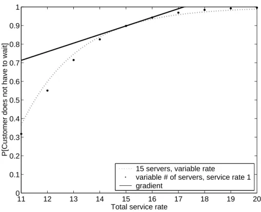
4.4 Performance as a function of service rate and as a function of the number of servers in anM/M/s queue. . . 54

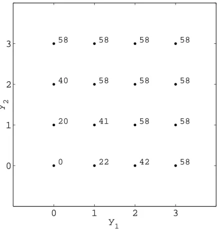
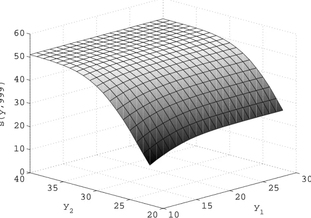
4.5 Sample average approximation (sample size 999) of the number of calls that are answered on time. . . 89

4.6 Subgradient estimates via the finite difference method. . . 90

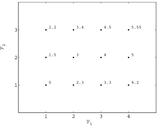
4.7 Subgradient estimates via the likelihood ratio method. . . 91

4.8 Subgradient estimates via IPA using a fixed number of servers. . . . 92

4.9 Subgradient estimates via IPA using a varying number of servers. . . 93

5.1 The analytic center cutting plane method (ACCPM). . . 100

5.2 (a) The sample average (sample sizen = 500) of the number of calls answered on time in period 2 as a function of the staffing levels in periods 1 and 2. (b) The contours of the service level function in (a). 105 5.3 Illustration of the feasible region and an iterate in the SACCPM. . . 108

5.4 The simulation-based analytic center cutting plane method (SAC-CPM). . . 109

5.5 The arrival rate function of Example 1. . . 118

5.6 The iterates of Experiment 1. . . 122

5.7 The optimality gap in Experiment 1. . . 122

5.8 The iterates of Experiment 2. . . 123

5.9 The optimality gap in Experiment 2. . . 123

5.10 Example 1: No shifts. . . 124

(9)

LIST OF TABLES

3.1 The iterates of the SKCPM. . . 42

3.2 The resulting service level function values of the iterates displayed in Table 3.1 and their 95% confidence intervals (CI). . . 42

3.3 Concavity study. . . 42

5.1 Different methods for adjusting the arrival rate to use in Equation (5.11). . . 114

5.2 The parameter settings in Example 2. . . 126

5.3 The experiments of Example 2. . . 129

5.4 Cost of the solutions in Example 2. . . 131

5.5 Feasibility of the solutions in Example 2. . . 132

5.6 Number of iterations in SACCPM-FD and SACCPM-IPA in Example 2. . . 133

(10)

LIST OF APPENDICES

A. PROOFS OF SOME OF THE IPA RESULTS AND TWO

IPA ALGORITHMS . . . 139

(11)

CHAPTER I

INTRODUCTION

Computer simulation is a powerful tool for analyzing a complex system. Infor-mation about the system can be obtained through a computer model without having to make costly experiments on the real system. When a decision needs to be made about the operating policies and settings of the system, some form of optimization is required. If there are only a few possible alternatives then it may be feasible to simulate the system at each different setting in order to determine which is the best one. In other cases, the computational time needed for such total enumeration is prohibitive. Then a more sophisticated optimization technique is required.

Linear integer programming problems, along with many other mathematical pro-gramming models, are well studied and many algorithms have been developed for solving problems in this form, but a simplification of the system is often required for modeling. In general, these methods cannot be applied when the performance of the model is evaluated by simulation. Therefore, optimization with simulation when there is a large number of possible alternatives is difficult. The existing methods for optimization with simulation include such heuristics as simulated annealing and tabu search. They require little or no structure of the underlying problem, but do not fully utilize such structure when it exists.

In this dissertation we develop methods for exploiting concavity properties, or more generally, pseudoconcavity properties, of the underlying problem in order to find a good solution more efficiently. By exploiting the structure of the underlying problem

(12)

we are also able to make stronger statements about the quality of the solutions we get than the aforementioned heuristics can.

The general framework of the methods is as follows: first, we solve a mathematical program to get an initial candidate solution. A simulation is run with the solution as an input to get information about the system performance. The information from the simulation at the candidate solution is used to build additional constraints into the mathematical program. We re-solve the mathematical program to get a new candidate solution and repeat the process until some stopping criteria are satisfied.

These methods are designed to solve problems where simulation may be the only viable option for estimating system performance and a decision is chosen from a large number of possible alternative system configurations. Additionally, the performance measure should at least approximately satisfy the pseudoconcavity property.

The method of combining simulation and optimization in this way has potential applications in various service systems, such as call center staffing and emergency vehicle dispatching. In fact, the method could potentially, with proper modifications, be utilized in many other areas where simulation is an appropriate modeling tool. In this thesis we focus our attention on the inbound call center staffing problem of scheduling workers at a minimum cost, while satisfying some minimum service level requirements.

The call center staffing problem has received a great deal of attention in the literature, and so one can reasonably ask why there is a need for a computational tool of this sort. To answer that question we first need to describe the overall staffing process. There are variations on the following theme (e.g., Castillo et al., 2003), but the essential structure is sequential in nature and is as follows (Mason et al., 1998).

1. (Forecasting) Obtain forecasts of customer load over the planning horizon, which is typically one or two weeks long. The horizon is usually broken into short periods that are typically between 15 minutes and 1 hour long.

(13)

2. (Work requirements) Determine the minimum number of agents needed dur-ing each period to ensure satisfactory customer service. Service is typically measured in terms of customer waiting times and/or abandonment rates in the queue.

3. (Shift construction) Select staff shifts that cover the requirements. This problem is usually solved through a set-covering integer program; see Mason et al. (1998) for more details.

4. (Rostering) Allocate employees to the shifts.

The focus in this thesis is on Steps 2 and 3. Steps 1 and 4 are not considered further. Step 2 is usually accomplished through the use of analytical results for simple queuing models. Green et al. (2001) coined the term SIPP (stationary, independent, period by period) to describe the general approach. In the SIPP approach, each period of the day is considered independently of other periods, the arrival process is considered to be stationary in that period, and one approximates performance in the period by a steady-state performance measure that is usually easily obtained from analytical results for particular queuing models. Heuristics are used to select input parameters for each period that yield a close match between the predictions and reality. For a wide variety of queuing models, this procedure results in some form of the “square-root rule,” which is a rule of thumb that provides surprisingly successful staffing level suggestions. See, e.g., Borst et al. (2004); Kolesar and Green (1998); Jennings et al. (1996) for more on the square-root rule.

The SIPP approach is appealing from the standpoint of computational tractability and due to the insights it provides. However, there are cases where the SIPP approach does not do as well as one might hope (Green et al., 2001, 2003). This can occur, for example, when the use of steady-state measures to represent performance over a short period is inappropriate. See Whitt (1991) for more on this point. Moreover,

(14)

call centers can be somewhat complex in structure, and this complexity can make it difficult to identify a queuing model of the center that is both mathematically tractable and a reasonable match to the true system. In such cases, simulation is a viable alternative. Indeed, simulation is now increasingly used in Step 2 (see Section VIII of Mandelbaum, 2003, for many examples) and commercial simulation packages, specially designed for call centers (e.g., Rockwell Software’s Arena Contact Center Edition), are available.

Further motivation for the use of simulation involves the linkage between staffing decisions in adjacent periods. Boosting staffing levels in one period can often help in reducing workload in subsequent periods, so that there can be linkage in perfor-mance between different periods. Such linkage can imply that there are multiple solutions to the work requirements problem that can offer valuable flexibility in Step 3. Traditional queuing approaches are not satisfactory in the presence of such link-age between periods, and in such cases one turns to simulation or other numerical methods. Indeed, Green et al. (2001, 2003) solve a system of ordinary differential equations through numerical integration to get the “exact” results for their models in order to compare the performance of various heuristics.

Assuming that one uses simulation or some other numerical method to predict performance in the call center, one then needs to devise a method to guide the selection of potential staffing levels to be evaluated through simulation. There have been several suggestions in the literature, all of which explicitly capture the linkage between periods in an attempt to realize cost savings. Like Green et al. (2001, 2003), Ingolfsson et al. (2002) use numerical integration to compute service level performance for a proposed set of staffing levels, and a genetic algorithm to guide the search. Ingolfsson et al. (2003) again use a numerical method to compute service level performance, and integer programming to guide the search. Castillo et al. (2003) devise a method for randomly generating sets of staff shifts that can be expected to perform well,

(15)

then use simulation to evaluate the service level performance of each set of generated staff shifts, and finally, plot the cost versus service level of the potential solutions to identify an efficient frontier. Henderson and Mason (1998) proposed a method that uses simulation to evaluate service level performance of a proposed set of shifts, and uses integer programming in conjunction with Kelley’s (Kelley, Jr., 1960) cutting plane method to guide the search.

1.1 Dissertation Outline

In Chapter II we formulate the problem of minimizing staffing costs in a call center while maintaining an acceptable level of service. The service level in the call center is estimated via simulation, so the call center staffing problem is then a simulation optimization problem. We adopt the “sample-average approximation” (SAA) ap-proach (see Shapiro, 2003; Kleywegt et al., 2001) for solving simulation-optimization problems. This approach, specialized to our setting, is as follows. One first gener-ates the simulation input data forn independent replications of the operations of the call center over the planning horizon. This data includes call arrival times, service times and so forth. The simulation data is fixed, and one then solves a determinis-tic optimization problem that chooses staffing levels so as to minimize staffing cost, while ensuring that average service computed only over the generated realizations is satisfactory.

Solving the SAA problem is non-trivial, since each function evaluation requires a simulation. In Chapter III we combine the cutting plane method of Henderson and Mason (1998) with the sample average approximation approach in the simulation-based Kelley’s cutting plane method (SKCPM). We establish its convergence prop-erties and give an implementation. This implementation identified two of the key issues, to be discussed next, of the cutting plane method and motivated the research in Chapters IV and V.

(16)

First, the method requires some form of gradient information to generate the cutting planes. The service level functions are discrete and, therefore, a gradient does not exist. Furthermore, the functions are estimated via simulation, so an analytical expression of the functions are not available. In Chapter IV we discuss the three most prominent gradient estimation techniques in the simulation literature: the method of finite differences, the likelihood ratio method and infinitesimal perturbation analysis. We show how each method can be applied in our setting and compare the three methods through a numerical example. The finite difference method gives the best gradient estimates, but is at the same time the most computationally expensive.

Second, the approach in Chapter III relies on an assumption that service in a period is concave and componentwise-increasing as a function of the staffing level vector. To understand this assumption, consider a single period problem. Increasing the staffing level should lead to improved performance. Furthermore, one might expect “diminishing returns” as the staffing level increases, so that performance would be concave in staffing level. Empirical results suggest that this intuition is correct, at least for sufficiently high staffing levels. But for low staffing levels, the empirical results suggest that performance is increasing and convex in the staffing level. So performance appears to follow an “S-shaped” curve (see Ingolfsson et al., 2003, and Chapter III) in one dimension. This non-concavity can cause the SKCPM to cut off feasible solutions, and the problem can be so severe as to lead to the algorithm suggesting impractical staffing plans. Nevertheless, the ability of the SKCPM to efficiently sift through the combinatorially huge number of potential staffing plans is appealing.

One might ask whether there is a similar optimization approach that can efficiently search through alternative staffing plans while satisfactorily dealing with S-shaped curves and their multidimensional extensions. In Chapter V we combine a relaxation on the assumption of concavity, i.e., pseudoconcavity, and additional techniques to

(17)

handle both the S-shaped curves alluded to above, as well as multidimensional be-havior seen in the numerical experiments (see, e.g., Figure 5.2). We developed the simulation-based analytic center cutting plane method for solving the SAA of the call center staffing problem. We prove under which conditions the method converges and include extensive numerical experiments, which show that the method is a robust one and often outperforms the traditional heuristics based on analytical queuing methods. Finally, in Chapter VI we provide concluding remarks and some directions for future research related to this thesis.

1.2 Contribution

We view the primary contributions of the dissertation as follows.

1. We demonstrate the potential of bringing simulation and traditional optimiza-tion methods together. Our methods are developed for the call center staffing problem, but our ideas and results will hopefully push research along these lines in other application areas.

2. We apply the method to the call center staffing problem, and our research lends valuable insight into the problem of scheduling employees at a low cost while maintaining an acceptable level of service, by identifying, and tackling, many of the key difficulties in the problem. Our computational results further indicate that the analytic center cutting plane method in Chapter V can be useful when traditional staffing methods fail.

3. The implementation of the methods is a challenging task. There is no standard software package that combines simulation and optimization in this way. Our successful implementation should be encouraging for other researchers as well as for makers of simulation and optimization software.

(18)

CHAPTER II

PROBLEM FORMULATION AND SAMPLE AVERAGE

APPROXIMATION

2.1 Introduction

In this chapter we formulate the call center staffing problem that serves as a moti-vating example for our work. We consider the problem of minimizing staffing costs while maintaining an acceptable level of service, where the service level can only be estimated via simulation. The random nature of the problem and the absence of an algebraic form for the service level function makes the optimization challenging. We use sampling to get an estimate of the service level function, and optimize over constraints on the sample average approximation (SAA). An important question is whether the solution to the sample average approximation problem converges to a solution to the original problem as the sample size increases, and if so, how fast.

We apply the strong law of large numbers to prove conditions for almost sure convergence and apply a result due to Dai et al. (2000) to prove an exponential rate of convergence of the optimal solutions as the sample size increases. Vogel (1994) proved almost sure convergence in a similar setting, but we include proofs for reasons listed in Section 2.3.1. Kleywegt et al. (2001) established conditions for an exponen-tial rate of convergence of the probability that the solution to the SAA problem is exactly the solution to the original discrete optimization problem when the expected value is in the objective. Vogel (1988) proved a polynomial rate of convergence in a similar setting, but under weaker conditions than we require. Homem-de-Mello

(19)

(2003) established convergence results for a variable sample method, which is similar to the SAA approach, but uses a different sample for each function evaluation. The optimization of SAA problems has also been studied in the simulation context (Chen and Schmeiser, 2001; Healy and Schruben, 1991; Robinson, 1996; Rubenstein and Shapiro, 1993).

The chapter is organized as follows. We formulate the call center staffing problem and its sample average approximation in Section 2.2. The convergence and the rate of convergence of the solutions of the SAA problem to solutions of the original problem are proved in Section 2.3.

2.2 Formulation of the Call Center Staffing

Prob-lem

The problem of determining optimal staffing levels in a call center (see, e.g., Thomp-son, 1997) is a motivating example for our work. We consider a somewhat simplified version of the real world problem for the purpose of developing the theory. We as-sume, for instance, that there is an unlimited number of trunk lines, one customer class, one type of agent and no abandonments. The decision maker faces the task of creating a collection of tours (work schedules) of low cost that together ensure a satisfactory service level.

A tour is comprised of several shifts and has to observe several restrictions related to labor contracts, management policies, etc. We divide the planning horizon (typ-ically a day or a week) into small periods (15-60 minutes). The set of permissible tours can be conveniently set up in a matrix (see Dantzig, 1954). More specifically we have Aij =     

1 if periodi is included in tourj

0 otherwise.

(20)

A represents a specific period. We let p be the total number of periods and m be the number of feasible tours. If we let x ∈Zm

+ be a vector where the jth component

represents the number of employees that work tour j, then Ax =y∈ Zp₊ is a vector where the ith _{component of} _y _{corresponds to the number of employees that work in} period i. We make the following natural assumption that every period is covered by at least one tour.

Assumption 2.1. For every periodi there is at least one tour j such thatAij = 1. The cost function is usually relatively straightforward to calculate. We can calcu-late the cost of each tour (salary costs, appeal to employees, etc.), and multiply by the number of employees working each tour to get the overall cost. Let cbe the cost vector, where cj is the cost per employee working tour j. Define the cost function

f(y) = min cT_x s.t. Ax ≥y

x ≥0 and integer.

(2.1)

It follows by Assumption 2.1 that (2.1) is feasible for any y. The value f(y) gives the minimum cost set of shifts that can cover the desired work requirements vector

y. We make the following assumption on the cost vector.

Assumption 2.2. The cost vector cis positive and integer valued.

Assumption 2.2 implies thatf(y) is integer valued and, moreover, sincecis positive and the entries in A are either 0 or 1, the z-level set of f,

{y≥0 and integer :∃x≥0 and integer, Ax≥y, cT_x_≤_z_}_, is finite for any z ∈R.

The management of a call center needs some criteria to follow when they decide on a set of staffing levels. It is not unusual in practice to determine the staffing levels from a service level perspective. In an emergency call center, for example, it might

(21)

be required that 90% of received calls should be answered within 10 seconds. We let

l ∈[0,1]p _{be the vector whose}_ith _{component is the minimum acceptable service level} in period i, e.g. 90%. Since, for example, the arrival and service times of customers are not known but are random, the service level in each period will be a random variable. Let Z, a random vector, denote all the random quantities in the problem and let z1_{, . . . , z}n _{denote independent realizations of} _Z_{. Let} _N

i(Z) be the number of calls received in period i and let Si(y, Z) be the number of those calls answered within a pre-specified time limit, for example 10 seconds, based on the staffing level

y. The fraction of customers receiving adequate service in period i in the long run is then lim n→∞ P_n d=1Si(y, zd) P_n d=1Ni(zd) = limn→∞n −1Pn d=1Si(y, zd) limn→∞n−1 P_n d=1Ni(zd) .

If E[Ni(Z)] <∞ then the strong law of large numbers can be applied separately to both the numerator and denominator of this expression, and then the desired long-run ratio isE[Si(y, Z)]/E[Ni(Z)]. Thus, E[Si(y, Z)]/E[Ni(Z)]≥li is a natural represen-tation of the service level constraint (excluding the pathological case E[Ni(Z)] = 0) in periodi. If we defineGi(y, Z) := Si(y, Z)−liNi(Z) then we can conveniently write the service level constraint as E[Gi(y, Z)]≥0. Define

gi(y) :=E[Gi(y, Z)] (2.2) as the expected service level in periodi as a function of the server allocation vectory

and let g :Rp _→_Rp _{be a function whose} _ith _{component is} _g

i. Finally, since an agent does not hang up on a call that he or she has already started working on we assume that if a server is still in service at the end of a period it finishes that service before becoming unavailable.

(22)

to satisfying a minimum service level in each period. It is min f(y)

subject to g(y) ≥ 0

y ≥ 0 and integer,

(2.3)

and note that problem (2.3) is equivalent to

min cT_x

subject to Ax ≥ y g(y) ≥ 0

x, y ≥ 0 and integer.

The functionsgi(y) are expected values, and the underlying model is typically so complex that an algebraic expression for g(y) can not be easily obtained. Therefore, simulation could be the only viable method for estimating g(y). In the next section we formulate an optimization problem which is an approximation of (2.3) obtained by replacing the expected values by sample averages and prove statements about the solutions of the approximation problem as solutions of the original problem (2.3).

2.3 Sample Average Approximation of the Call

Center Staffing Problem

In this thesis we assume that the algebraic form of the service level function g(y) is not available, and that its value is estimated using simulation. Suppose we run a simulation with sample size n, where we independently generate the realizations {zd_}n

d=1 from the distribution of Z, to get an estimate of the expected value of g(y).

Let ¯ g(y;n) = 1 n n X d=1 G(y, zd)

be the resulting estimates and let ¯gi(y;n) denote the ith _{component of ¯}_g₍_y_;_n_{). We} use this notation to formulate the SAA problem

(23)

min f(y)

subject to g¯(y;n) ≥ 0

y ≥ 0 and integer.

(2.4)

In Section 2.3.1 we show, by using the strong law of large numbers (SLLN), that the set of optimal solutions of the SAA problem (2.4) is a subset of the set of optimal solutions for the original problem (2.3) with probability 1 (w.p.1) as the sample size gets large. Furthermore, we show in Section 2.3.2 that the probability of this event approaches 1 exponentially fast when we increase the sample size. These results require the existence of at least one optimal solution for the original problem to satisfy the expected service level constraints with strict inequality, but this regularity condition can be easily justified for practical purposes as will be discussed later.

2.3.1 Almost Sure Convergence of Optimal Solutions of the

Sample Average Approximation Problem

The results in this section may be established by specializing the results in Vogel (1994). We choose to provide direct proofs in this section for 3 main reasons:

1. The additional structure in our setting allows a clearer statement and proof of the results.

2. The proofs add important insight into why solving the SAA problem is a sensible approach.

3. The proofs serve as an excellent foundation to develop an understanding of the “rate of convergence” results that follow in Section 2.3.2.

We are interested in the properties of the optimal solutions of (2.4) as the sample size n gets large. It turns out, by an application of the SLLN, that any optimal solution of (2.3) that satisfies g(y)>0, i.e., gi(y)>0 for alli, is an optimal solution

(24)

of (2.4) with probability 1 (w.p.1) as n goes to infinity. We introduce additional notation before we prove this. Let

¯

g(y;∞) := limn→∞¯g(y;n),

F∗ _{:= the optimal value of (2.3)} and define the sets

Y∗ _{:= the set of optimal solutions to (2.3),}

Y∗

0 := {y∈Y∗ :g(y)>0},

Y1 := {y∈Zp+ :f(y)≤F∗, g(y)0},

Y∗

n := the set of optimal solutions to (2.4).

Note that Y1 is the set of solutions to (2.3) that have the same or lower cost than

an optimal solution, and satisfy all constraints except the service level constraints. We are concerned with solutions in this set since they could be feasible (optimal) for the SAA problem (2.4) if the difference between the sample average, ¯g(·;n), and g is sufficiently large. We show that when Y∗

0 is not empty, Y0∗ ⊆Yn∗ ⊆Y∗ for all n large enough w.p.1.1 _{The sets}_Y∗_, _Y∗

n and Y0∗ are finite by Assumption 2.2. (The sets Y∗,

Y∗

n and Y0∗ can be empty). Furthermore, if Y∗ is nonempty then F∗ <∞ and then,

again by Assumption 2.2, the set Y1 is finite.

We start with two lemmas. The first one establishes properties of ¯g(y;∞) by repeatedly applying the SLLN. The second shows that solutions to (2.3) satisfying

g(y) > 0, and infeasible solutions, will be feasible and infeasible, respectively, w.p.1 for problem (2.4) when n gets large. The only condition g(y) has to satisfy is that it has to be finite for all y ∈ Zp₊. That assumption is easily justified by noting that the absolute value of each component of g(y) is bounded by the expected number of

1_{We say that property}_E₍_n_{) holds for all} _n_{large enough w.p.1 if and only if} _P_[_∃_{N <}_∞_:_E₍_n₎

holds∀n≥N] = 1. (HereN should be viewed as a random variable.) Sometimes such statements are communicated by saying thatE(n) holdseventually.

(25)

arrivals in that period, which would invariably be finite in practice. Define kgk= max y∈Zp+ kg(y)k∞= max y∈Zp+ max i=1,...,p|gi(y)|. Lemma 2.1.

1. Suppose that kg(y)k∞ <∞ for some fixedy ∈Z₊p. Then g¯(y;∞) =g(y) w.p.1. 2. Suppose that kgk < ∞ and Γ ⊂ Zp₊ is finite. Then ¯g(y;∞) = g(y) ∀ y ∈ Γ

w.p.1.

Proof:

1. The SLLN (Theorem B.1) gives ¯gi(y;∞) = gi(y) w.p.1. SoP[¯g(y;∞) =g(y)]≥ 1−Pp_i₌₁P[¯gi(y;∞)6=gi(y)] = 1 by Boole’s inequality; see Equation (B.1). 2. Note that P[¯g(y;∞) = g(y) ∀ y ∈ Γ]≥ 1−P_y∈_ΓP[¯g(y;∞)6= g(y)] = 1 since

Γ is finite.

Lemma 2.2. Suppose that kgk<∞ and that Assumption 2.2 holds. Then 1. g¯(y;n)≥0∀y∈Y∗

0 for all n large enough w.p.1.

2. Ally ∈Y1 are infeasible for the SAA problem (2.4) for all n large enough w.p.1

if F∗ _<_∞_.

Proof:

1. The result is trivial if Y∗

0 is empty, so suppose it is not. Let

²= min y∈Y∗ 0

min

i∈{1,...,p}{gi(y)}. Then ² >0 by the definition of Y∗

0. Let N0 = inf{n0 : max y∈Y∗ 0 k¯g(y;n)−g(y)k∞< ²∀n≥n0}. Then ¯g(y;n)≥0∀y ∈Y∗

0 ∀ n≥ N0. The set Y0∗ is finite, so limn→∞g¯(y;n) =

g(y)∀y∈Y∗

(26)

2. The result is trivial if Y1 is empty, so suppose it is not. Let

²= min y∈Y1

max

i∈{1,...,p}{−gi(y)}.

Then ² >0, sincegi(y)<0, for at least one i∈ {1, . . . , p} ∀y∈Y1. Let

N1 = inf{n1 : max

y∈Y1

kg(y)−g¯(y;n)k∞ < ²∀n ≥n1}

and then ally ∈Y1 are infeasible for (2.4) for alln ≥N1. The set Y1 is a finite

by Assumption 2.2 and since F∗ _<_{∞, so} lim

n→∞¯g(y;n) = g(y)∀y ∈Y1 w.p.1 by part 2 of Lemma 2.1. Therefore, N1 <∞ w.p.1.

Lemma 2.2 shows that all the “interior” optimal solutions for the original problem are eventually feasible for the SAA problem and remain so as the sample size increases. Furthermore, all solutions that satisfy the constraints that are common for both problems, but not the service level constraints, and have at most the same cost as an optimal solution, eventually become infeasible for the SAA problem. Hence, we have the important result that for a large enough sample size an optimal solution for the SAA problem is indeed optimal for the original problem.

Theorem 2.3. Suppose thatkgk<∞and that Assumption 2.2 holds. ThenY∗

0 ⊆Yn∗

for all n large enough w.p.1. Furthermore, if Y∗

0 is nonempty thenY0∗ ⊆Yn∗ ⊆Y∗ for

all n large enough w.p.1.

Proof: The first inclusion holds trivially if Y∗

0 is empty, so assume that Y0∗ is not

empty, and henceF∗ _<_{∞. On each sample path let}_N _{= sup{}_N

0, N1}, whereN0 and

N1 are the same as in Lemma 2.2. Whenn≥N we know that all y∈Y0∗ are feasible

for (2.4) and that all y ∈ Y1 are infeasible for (2.4). Hence, all y ∈ Y0∗ are optimal

for (2.4) and no y 6∈ Y∗ _{is optimal for (2.4) whenever} _n _≥ _N_{. Thus,} _Y∗

0 ⊆ Yn∗ ⊆ Y∗ for all n ≥ N. Finally, P[N <∞] = P[N < ∞, N < ∞] ≥ P[N < ∞] +P[N <

(27)

∞]−1 = 1.

Corollary 2.4. Suppose that kgk < ∞, Assumption 2.2 holds and that (2.3) has a unique optimal solution, y∗_{, such that} _g₍_y∗₎ _> ₀_{. Then} _y∗ _{is the unique optimal}

solution for (2.4) for all n large enough w.p.1.

Proof: In this case Y∗

0 =Y∗ ={y∗} and the result follows from Theorem 2.3.

The conclusion of Theorem 2.3 relies on existence of an “interior” optimal solution for the original problem. A simple example illustrates how the conclusion can fail if this requirement is not satisfied. Let Z be a uniform random variable on [−0.5,0.5] and consider the following problem:

min y

subject to y ≥ |E[Z]|

y ≥ 0 and integer.

Theny∗ _{= 0 for this problem since}_E_[_Z_{] = 0. We form the SAA problem by replacing}

E[Z] with ¯Z(n), the sample average of n independent realizations of Z. Then 0.5 >

|Z¯(n)|>0 w.p.1 for all n >0 and thus we get that y∗

n = 1 w.p.1.

Remark 2.1. The existence of an “interior” optimal solution is merely a regularity condition. In reality it is basically impossible to satisfy the service level constraints in any period exactly, since the feasible region is discrete. Even if this occurred, we could subtract an arbitrarily small positive number, say ε, from the right hand side of each service level constraint and solve the resulting ε-perturbed problem. Then all solutions with gi(y) = 0 for some i satisfy gi(y) > −ε and it is sufficient for the problem to have an optimal solution (not necessarily satisfying g(y) > 0) for Theorem 2.3 to hold.

Remark 2.2. It may possible to replace the constraint ¯g(y;n) ≥ 0 with ¯g(y;n) ≥ −ε(n), and prove a similar result as in Theorem 2.3 under stronger conditions on

g(y), by letting ε(n)→0 at a slow enough rate as n→ ∞.

Remark 2.1 also applies in the next subsection where we prove an exponential rate of convergence as the sample size increases.

(28)

2.3.2 Exponential Rate of Convergence of Optimal Solutions

of the Sampled Problems

In the previous subsection we showed that we can expect to get an optimal solution for the original problem (2.3) by solving the SAA problem (2.4) if we choose a large sample size. In this section we show that the probability of getting an optimal solution this way approaches 1 exponentially fast as we increase the sample size. We use large deviations theory and a result due to Dai et al. (2000) to prove our statement. Vogel (1988) shows, under weaker conditions, that the feasible region of a sample average approximation of a chance constraint problem approaches the true feasible region at a polynomial rate and conjectures, without giving a proof, that an exponential rate of convergence is attainable under similar conditions to those we impose.

The following theorem is an intermediate result from Theorem 3.1 in Dai et al. (2000):

Theorem 2.5. Let H : Rp_×_Ω _→_R _{and assume that there exist} _{γ >} ₀_, _θ

0 >0 and

η: Ω→R such that

|H(y, Z)| ≤γη(Z), E[eθη(Z)_]_<_∞_,

for all y∈ Rp _{and for all} ₀_≤ _θ _≤_θ

0, where Z is a random element taking values in

the space Ω. Then for any δ >0, there exist a >0, b >0, such that for any y∈Rp

P[|h(y)−¯h(y;n)| ≥δ]≤ae−bn_,

for alln >0, whereh(y) = E[H(y, Z)], andh¯(y;n)is a sample mean ofnindependent and identically distributed realizations of H(y, Z).

In our setting take H(y, Z) = Gi(y, Z) and note that |Gi(y, Z)| ≤ Ni(Z), where

Ni is the number of calls received in period i. If the arrival process is, for example, a (nonhomogeneous or homogeneous) Poisson process, which is commonly used to model incoming calls at a call center, then Ni satisfies the condition of Theorem 2.5 since it is a Poisson random variable, which has a finite moment generating function (Ross, 1996).

(29)

that for any n, Y∗

0 ⊆ Yn∗ ⊆ Y∗ precisely when all the solutions in Y0∗ are feasible for

the SAA problem and all infeasible solutions for (2.3) that are equally good or better, i.e., are in the set Y1, are also infeasible for (2.4).

Lemma 2.6. Let n >0be an arbitrary integer and let Y∗

0 be nonempty. The

proper-ties

1. g¯(y;n)≥0∀y∈Y∗

0, and

2. g¯(y;n)0∀y∈Y1

hold if and only if Y∗

0 ⊆Yn∗ ⊆Y∗.

Proof: Suppose properties 1 and 2 hold. Then by property 1 ally∈Y∗

0 are feasible

for (2.4) and the optimal value of (2.4) is at most F∗ _since _Y∗

0 is nonempty. By

property2 there are no solutions with a lower objective that are feasible for (2.4), so

Y∗

0 ⊆ Yn∗. By property 2, no solutions outside Y∗ with objective value equal to F∗ are feasible for (2.4). Hence, Y∗

0 ⊆Yn∗ ⊆Y∗. Suppose Y∗

0 ⊆ Yn∗ ⊆ Y∗. Then F∗ is the optimal value for (2.4). Now, since all

y∈Y∗

0 are optimal for (2.4) they are also feasible for (2.4) and property 1 holds. All

y∈Y1 are infeasible for (2.4) since Yn∗ ⊆Y∗ and therefore property 2 holds.

Theorem 2.7. Suppose Gi(y, Z) satisfies the assumptions of Theorem 2.5 for all

i ∈ {1, . . . , p}, Assumption 2.2 holds and that Y∗

0 is nonempty. Then there exist

α >0, β >0 such that P[Y∗ 0 ⊆Yn∗ ⊆Y∗]≥1−αe−βn. Proof: Define δ1 := min y∈Y∗ 0 min i∈{1,...,p}{gi(y)}, i(y) := arg max i∈{1,...,p}{−gi(y)}, δ2 := min y∈Y1 {−gi(y)(y)}, and δ:= min{δ1, δ2}.

(30)

Here δ1 > 0 is the minimal amount of slack in the constraints “g(y) ≥ 0” for any

solution y∈Y∗

0. Similarly δ2 >0 is the minimal violation in the constraints “g(y)≥

0” induced by any solution y∈Y1. Thus,

P[Y₀∗ ⊆Y_n∗ ⊆Y∗] =P[¯g(y;n)≥0∀y∈Y∗ 0,g¯(y;n)0∀y∈Y1] (2.5) = 1−P[¯g(y;n)0 for somey ∈Y∗ 0 or ¯g(y;n)≥0 for some y∈Y1] ≥1− X y∈Y∗ 0 p X i=1 P[¯gi(y;n)<0]− X y∈Y1 P[¯g(y;n)≥0] (2.6) ≥1− X y∈Y∗ 0 p X i=1 P[|¯gi(y;n)−gi(y)| ≥δ]− X y∈Y1 P[|¯gi(y)(y;n)−gi(y)(y)| ≥δ] (2.7) ≥1− X y∈Y∗ 0 p X i=1 aie−bin− X y∈Y1 ai(y)e−bi(y)n (2.8) ≥1−αe−βn. Here α =|Y∗ 0| P_p i=1ai+ P

y∈Y1ai(y) and β = mini∈{1,...,p}bi, where |Y ∗

0| is the

cardi-nality of the set Y∗

0. The sets Y0∗ and Y1 are finite by Assumption 2.2, so α < ∞.

Equation (2.5) follows by Lemma 2.6. Equation (2.6) is Boole’s inequality; see (B.1). Equation (2.7) follows since P[¯g(y;n) ≥ 0] ≤ P[¯gi(y)(y;n) ≥ 0] and gi(y) ≥ δ1 ≥ δ

for y ∈ Y∗

0 and gi(y)(y) ≥ δ2 ≥ δ for y ∈ Y1. Equation (2.8) follows from Theorem

2.5.

The case where Y∗

0 is empty but Y∗ is not would almost certainly never arise in

practice. But in such a case one can solve an ε-perturbation of (2.4) as described in Remark 2.1, and the results of Theorem 2.7 hold for 0 ≤ε < δ.

Justified by the results of this chapter, in the remainder of the thesis we discuss how to solve the SAA problem (2.4).

(31)

CHAPTER III

THE SIMULATION-BASED KELLEY’S CUTTING

PLANE METHOD

3.1 Introduction

In Chapter II we formulated the call center staffing problem (2.3) and its sample average approximation (SAA) problem (2.4). In this chapter we present a conceptual cutting plane method for solving the SAA problem. This method was proposed by Henderson and Mason (1998) and combines simulation and integer programming in an iterative cutting plane algorithm. The algorithm relies on the concavity of the problem constraints, but in our algorithm we have a built-in subroutine for detecting nonconcavity, so the method is robust.

The method is based on the one developed by Kelley, Jr. (1960) and solves a linear (integer) program to obtain the staffing levels, and the solution is used as an input for a simulation to calculate the service level. If the service level is unsatisfactory, a constraint is added to the linear program and the process is repeated. If the service level is satisfactory the algorithm terminates with an optimal solution of the SAA problem.

Kelley’s cutting plane method applies to minimization problems where both the objective function and feasible region (of the continuous relaxation of the integer problem) need to be convex. The costs in the call center problem are linear and we assume that the service level function is concave, so that (see Equation (2.3)), the feasible region, relaxing the integer restriction, is convex. Since the service level

(32)

function is unknown beforehand, we need to incorporate a mechanism into the method to verify that the concavity assumption holds. In Section 3.4 we present a numerical method for checking concavity of a function, when the function values and, possibly, gradients are only known at a finite number of points.

Cutting plane methods have been successfully used to solve two stage stochas-tic linear programs. In many applications the sample space becomes so large that one must revert to sampling to get a solution (Birge and Louveaux, 1997; Infanger, 1994). The general cutting plane algorithm for two stage stochastic programming is known as the L-Shaped method (van Slyke and Wets, 1969) and is based on Benders decomposition (Benders, 1962). Stochastic Decomposition (Higle and Sen, 1991) for solving the two stage stochastic linear program starts with a small sample size, which is increased as the algorithm progresses and gets closer to a good solution. Stochastic Decomposition could also be applied in our setting, but that is not within the scope of this thesis.

Morito et al. (1999) use simulation in a cutting-plane algorithm to solve a logistic system design problem at the Japanese Postal Service. Their problem is to decide where to sort mail provided that some post offices have automatic sorting machines but an increase in transportation cost and handling is expected when the sorting is more centralized. The algorithm proved to be effective for this particular problem and found an optimal solution in only 3 iterations where the number of possible patterns (where to sort mail for each office) was 230_{. Their discussion of the algorithm is ad}

hoc, and they do not discuss its convergence properties.

Koole and van der Sluis (2003) developed a local search algorithm for a call cen-ter staffing problem with a global service level constraint. When the service level constraint satisfies a property called multimodularity their algorithm is guaranteed to terminate with a global optimal solution. There are, however, examples where the service level constraint, as defined in Chapter II, is not multimodular even for

(33)

nondecreasing and concave service level functions.

The chapter is organized as follows. In Section 3.2 we discuss the concavity as-sumption in more detail. We present the cutting plane algorithm and its convergence properties in Section 3.3. The numerical method for checking concavity is described in Section 3.4 and an implementation of the overall method is described in Section 3.5.

3.2 Concave Service Levels and Subgradients

Intuitively, we would expect that the service level increases if we increase the number of employees in any given period. We also conjecture that the marginal increase in service level decreases as we add more employees. If these speculations are true then

gi(y) is increasing and concave in each component ofyfor alli. In this chapter, we will make the stronger assumption that gi(y) and ¯gi(y;n) are increasing componentwise and jointly concave in y, for alli. Our initial computational results suggest that this is a reasonable assumption, at least within a region containing practical values of y

(see Section 3.5). Others have also studied the convexity of performance measures of queuing systems. Ak¸sin and Harker (2001) show that the throughput of a call center is stochastically increasing and directional concave in the sample path sense as a function of the allocation vector y in a similar setting. Analysis of the steady state waiting time of customers in an M/M/squeue shows that its expected value is a convex and decreasing function of the number of servers s (Dyer and Proll, 1977), its expected value is convex and increasing as a function of the arrival rate (Chen and Henderson, 2001) and its distribution function evaluated at any fixed value of the waiting time, is concave and decreasing as a function of the arrival rate (Chen and Henderson, 2001). See other references in Chen and Henderson (2001) for further studies in this direction.

If the concavity assumption holds (we will discuss the validity of this assumption later), then we can approximate the service level function with piecewise linear

(34)

con-cave functions, which can be generated as described below. The following definition is useful:

Definition 3.1. (In Rockafellar, 1970, p. 308) Let ˆy ∈Rp _{be given and} _h _:_Rp _→_R be concave. The vector q(ˆy)∈Rp _{is called a} _subgradient _of _h _{at ˆ}_y _if

h(y)≤h(ˆy) +q(ˆy)T₍_y₋_y_ˆ₎_∀_y _∈_Rp_. _(3.1) The term “supergradient” might be more appropriate since the hyperplane

{(y, p(y)) :p(y) =h(ˆy) +q(ˆy)T₍_y₋_y_ˆ₎_∀_y_∈_R_}

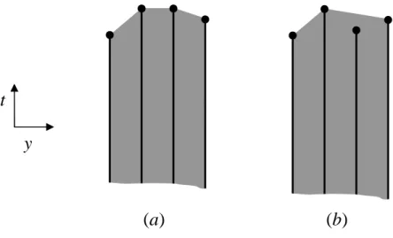
lies “above” the function h, but we use “subgradient” to conform with the literature. A concave function has at least one subgradient at every point in the interior of its convex domain (see Theorem 3.2.5 in Bazaraa et al., 1993). The notion of concavity and subgradients is defined for functions of continuous variables, but we are dealing with functions of integer variables here. Therefore, we need to define concavity of discrete functions; see the illustration in Figure 3.1.

Definition 3.2. The functionh:Zp _→_R_is _{discrete concave} _{if no points (}_{x, h}₍_x₎₎_∈

Zp_×_R _{lie in the interior of the set conv{(}_{y, t}_{) :}_y_∈_Zp_{, t}_∈_{R, t}_≤_h₍_y_)}.

Here, conv(S) is the convex hull of the set S, which is the smallest convex set containingS. Definition 3.2 is similar to the definition of a convex extensible function in Murota (2003, p. 93) when the function his finite. We define the subgradient of a discrete concave function as follows.

Definition 3.3. Let ˆy∈Zp _{be given and}_h_:_Zp _→_R_{be discrete concave. The vector}

q(ˆy)∈Zp _{is called a} _{subgradient of the discrete concave} _function_h _{at ˆ}_y _if

h(y)≤h(ˆy) +q(ˆy)T₍_y₋_y_ˆ₎_∀_y_∈_Zp_. _(3.2) A discrete concave function has a subgradient at every point by Theorem 2.4.7 in Bazaraa et al. (1993), since the set conv{(y, t) :y∈Zp_{, t}_∈_{R, t}_≤_h₍_y_)}_{is closed.}

Letqi(ˆy) and ¯qi(ˆy;n) be subgradients at ˆyofgi(y) and ¯gi(y;n), respectively. There are many potential methods one might consider to obtain the subgradients. Finite

(35)

(a)

(b)

y

t

Figure 3.1: Illustration of a discrete concave function. (a) discrete concave. (b) not discrete concave. The dots are points of the form (y, h(y)). The lines represent the points in the set {(y, t) : y ∈

Zp_{, t}_∈_R_{, t}_≤_h₍_y₎_} _{and the shaded area is the set conv}_{₍_{y, t}_{) :}_y_∈_Zp_{, t}_∈_R_{, t}_≤_h₍_y₎_}_.

differences using differences of length 1 appear reasonable since we are working with integer variables. There are, however, examples where that fails to produce a sub-gradient, even for a concave nondecreasing function. Still, we used finite differences in our numerical study and converged to an optimal solution of the SAA problem. Gradients might also be obtained using infinitesimal perturbation analysis (IPA) (see, e.g., Glasserman, 1991). Before using IPA we would have to extend the service level function to a differentiable function defined over a continuous domain, since IPA is applied in settings where the underlying function is differentiable. See Chapter IV for a detailed treatment.

The subgradients are used to approximate the sample average of the service level constraints. Let ˆy be a given server allocation vector, and suppose that ¯gi(ˆy;n) and ¯

qi(ˆy;n) are as above. If our assumptions about concavity of ¯ghold, then by Definition 3.3 we must have ¯gi(y;n)≤g¯i(ˆy;n) + ¯qi(ˆy;n)T(y−yˆ) for all allocation vectorsy, and all i. We wanty to satisfy ¯g(y;n)≥0 and therefore it is necessary that

0≤g¯i(ˆy;n) + ¯qi(ˆy;n)T(y−yˆ), (3.3) for all i.

(36)

3.3 The Simulation-Based Kelley’s Cutting Plane

Method

In this section we present a cutting plane algorithm for solving the SAA problem (2.4).

To make the presentation of our algorithm clearer and to establish the convergence results we make the following assumption on the tour vector x.

Assumption 3.1. The tour vector x is restricted to a compact setX.

The above assumption can be easily justified in practice. It is, for example, impossible to hire an infinite number of employees, and there are usually budget constraints which impose an upper bound onx sincecis positive by Assumption 2.2. Under Assumption 3.1 the original problem (2.3) becomes

min cT_x subject to Ax ≥ y g(y) ≥ 0 x ∈ X x, y ≥ 0 and integer, (3.4)

and the sample average approximation of (3.4) is

min cT_x subject to Ax ≥ y ¯ g(y;n) ≥ 0 x ∈ X x, y ≥ 0 and integer. (3.5)

The results of Section 2.3 for the optimal solutions of (2.3) and (2.4) still hold for problems (3.4) and (3.5) if Y∗ _and _Y∗

n are defined as the sets of optimal solutions of (3.4) and (3.5), respectively.

(37)

We also define, for future reference,

Y :={y≥0 and integer :∃0≤x∈X and integer with Ax≥y}. (3.6) This is the set of staffing levels y that satisfy all the constraints in (3.4) except the expected service level constraints. Note that Y is a finite set since X is compact and the entries in A are either 0 or 1.

Our algorithm fits the framework of Kelley’s cutting plane method (Kelley, Jr., 1960). We relax the nonlinear service level constraints of (3.5) to convert the call center staffing problem into a linear integer problem. We then solve the linear integer problem and run a simulation with the staffing levels obtained from the solution. If the service levels meet the service level constraints as approximated by the sample average then we stop with an optimal solution to (3.5). If a service level constraint is violated then we add a linear constraint to the relaxed problem that eliminates the current solution but does not eliminate any feasible solutions to the SAA problem. The procedure is then repeated.

Our algorithm differs from the traditional description of the algorithm only in that we use a simulation to generate the cuts and evaluate the function values instead of having an algebraic form for the function and using analytically determined gradients to generate the cuts. Nevertheless, we include a proof of convergence of our cutting plane method, since its statement is specific to our algorithm and it makes the results clearer.

The relaxed problem for (3.5) that we solve in each iteration is

min cT_x subject to Ax ≥ y Dk_y _≥ _dk x ∈ X x, y ≥ 0 and integer. (3.7)

(38)

The constraints ¯g(y;n) ≥ 0 have been replaced with linear constraints Dk_y _≥ _dk_. The superscriptk indicates the iteration number in the cutting plane algorithm. The constraint set Dk_y _≥ _dk _{is initially empty, but we add more constraints to it as the} algorithm progresses.

We select a fixed sample size, n, at the beginning of the algorithm and use the same sample (common random numbers) in each iteration. It is usually not necessary to store then independent realizations. Instead, we only need to store a few numbers, namely seeds, and reset the random number generators (streams) in the simulation with the stored seeds at the beginning of each iteration. See Law and Kelton (2000) for more details on this approach to using common random numbers. Using common random numbers minimizes the effect of sampling in that we only work with one function ¯g(·;n) instead of getting a new ¯g(·;n) function in each iteration, which could, for example, invalidate the concavity assumption.

At iteration k we solve an instance of (3.7) to obtain the solution pair (xk_{, y}k_). For the server allocation vector yk _{we run a simulation to calculate ¯}_g₍_yk_;_n_{). If we} find that the service level is unacceptable, i.e., if ¯gi(yk;n) < 0 for some i, then we add the constraint (3.3) to the setDk_y_≥_dk_{, i.e., we add the component}_−¯_g

i(yk;n) + ¯

qi(yk;n)Tyk to dk and the row vector ¯qi(yk;n)T to Dk. We add a constraint for all periods i where the service level is unacceptable. Otherwise, if the service level is acceptable in all periods, then we terminate the algorithm with an optimal solution to the SAA problem (3.5). We summarize the simulation-based Kelley’s plane method (SKCPM) for the call center staffing problem in Figure 3.2

To speed up the algorithm it is possible to start with D1 _and _d1 _nonempty.

In-golfsson et al. (2003) developed, for example, lower bounds ony. They point out that if there is an infinite number of servers in all periods except period i and if ˜yi is the minimum number of employees required in period iin this setting so that the service level in period i is acceptable, then yi ≥ y˜i for all y satisfying g(y) ≥ 0. We could

(39)

Initialization Generate n independent realizations from the distribution ofZ. Let

k := 1, D1 _and _d1 _{be empty.}

Step 1 Solve (3.7) and let (xk_{, y}k_{) be an optimal solution.}

Step 1a Stop with an error if (3.7) was infeasible.

Step 2 Run a simulation to obtain ¯g(yk_;_n_).

Step 2a If ¯g(yk_;_n₎_≥_{0 then stop. Return (}_xk_{, y}k_{) as a solution for (3.5).}

Step 3 Compute, by simulation, ¯qi(yk;n) for all i for which ¯gi(yk;n) < 0, and add the cuts (3.3) to Dk _and _dk_.

Step 4 Let dk+1 _:=_dk _and _Dk+1 _:=_Dk_{. Let} _k _:=_k_{+ 1. Go to Step 1.}

Figure 3.2: The simulation-based Kelley’s cutting plane method (SKCPM).

select D1 _and _d1 _{to reflect such lower bounds.}

If the SKCPM terminates in Step 1a then the SAA problem is infeasible. That could be due to either a sampling error, i.e., the SAA problem does not have any fea-sible points even though the original problem is feafea-sible, or that the original problem is infeasible. As a remedy, either the sample size should be increased, or the original problem should be reformulated, for example, by lowering the acceptable service level, or X should be expanded, e.g., by allocating more employees.

In the SKCPM an integer linear program is solved and constraints are added to it in each iteration until the algorithm terminates. The integer linear problem always has a larger feasible region than the SAA problem (3.5), so cT_xk _≤ _cT_xk+1 _≤ _cT_x∗

n, where (x∗

n, yn∗) is an optimal solution for (3.5). An important question is whether limk→∞cTxk =cTx∗n. The following theorem answers this question in the positive.

Theorem 3.1.

1. The algorithm terminates in a finite number of iterations.

2. Suppose that each component of g¯(y;n) is concave in y. Then the algorithm terminates with an optimal solution to (3.5) if and only if (3.5) has a feasible solution.