Input Window Size and Neural Network Predictors R.J.Frank, N.Davey, S.P.Hunt
University of Hertfordshire Hatfield, UK.
Email: { R.J.Frank, N.Davey, S.P.Hunt }@herts.ac.uk
Abstract
Neural Network approaches to time series prediction are briefly discussed, and the need to specify an appropriately sized input window identified. Relevant theoretical results from dynamic systems theory are briefly introduced, and heuristics for finding the correct embedding
dimension, and thence window size, are discussed. The method is applied to two time series and the resulting generalisation performance of the trained feed-forward neural network predictors is analysed. It is shown that the heuristics can provide useful information in
defining the appropriate network architecture.
1 INTRODUCTION
Neural Networks have been widely used as time series forecasters: most often these are feed-forward networks which employ a sliding window over the input sequence. Typical examples of this approach are market predictions, meteorological and network traffic forecasting. [1,2,3]. Two important issues must be addressed in such systems: the frequency with which data should be sampled, and the number of data points which should be used in the input representation. In most applications these issues are settled empirically, but results from work in complex dynamic systems suggest helpful heuristics. The work reported here is concerned with investigating the impact of using these heuristics. We attempt to answer the question: can the performance of sliding window feed-forward neural network predictors be optimised using theoretically motivated heuristics? We report experiments using two data sets: the sequence obtained from one of the three dimensions of the Lorenz attractor, and a series of 1500 tree ring measurements.
2 TIME SERIES PREDICTION
A time series is a sequence of vectors, x(t), t = 0,1,… , where t represents elapsed time.
For simplicity we will consider here only sequences of scalars, although the techniques considered generalise readily to vector series. Theoretically, x may be a value which varies continuously with t, such as a temperature. In practice, for any given physical system, x will be sampled to give a series of discrete data points, equally spaced in time. The rate at which samples are taken dictates the maximum resolution of the model; however, it is not always the case that the model with the highest resolution has the best predictive power, so that superior results may be obtained by employing only every nth point in the series. Further discussion of this issue, the choice of time lag, is delayed until section 3.2, and for the time being we assume that every data point collected will be used.
Work in neural networks has concentrated on forecasting future developments of the time series from values of x up to the current time. Formally this can be stated as: find a function f:ℜ → ℜ such as to obtainN an estimate of x at time t + d, from the N time steps back from time t, so that:
x t( +d)= f x t x t( ( ), ( −1),K, (x t− +N 1))
x t( +d)= f( ( ))yt where y( )t is the N - ary vector of lagged valuesx
Neural Network Predictors
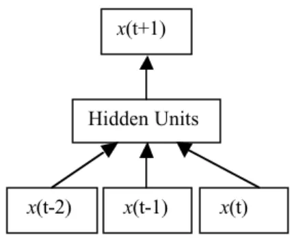
The standard neural network method of performing time series prediction is to induce the function ƒ in a standard MLP or an RBF architecture, using a set of N-tuples as inputs and a single output as the target value of the network. This method is often called the sliding window technique as the N-tuple input slides over the full training set. Figure 1 gives the basic architecture.
Figure 1: The standard method of performing time series prediction using a sliding window of, in this case, three time steps.
As noted in [4] this technique can be seen as an extension of auto-regressive time series modelling, in which the function ƒ is assumed to be a linear combination of a fixed number of previous series values. Such a restriction does not apply with the MLP approach as MLPs are general function approximators.
3 THEORETICAL CONSIDERATIONS
Time series are generally sequences of measurements of one or more visible variables of an underlying dynamic system, whose state changes with time as a function of its current state vector u(t):
d t dt G t u u ( ) ( ( )) =
For the discrete case, the next value of the state is a function of the current state: u(t+ =1) F( ( ))ut
Such dynamic systems may evolve over time to an attracting set of points that is regular and of simple shape; any time series derived from such a system would also have a smooth and regular appearance. However another result is possible: the system may evolve to a chaotic attractor. Here, the path of the state vector through the attractor is non-periodic and because of this any time series derived from it will have a complex appearance and behaviour.
In a real-world system such as a stock market, the nature and structure of the state space is obscure; so that the actual variables that contribute to the state vector are unknown or debatable. The task for a time series predictor can therefore be rephrased: given measurements of one component of the state vector of a dynamic system is it possible to reconstruct the (possibly) chaotic dynamics of the phase space and thereby predict the evolution of the measured variable? Surprisingly the answer to this is yes. The embedding theorem of Mañé & Takens [5] shows that the space of time lagged vectors y with sufficiently large dimension will capture the structure of the original phase space. More specifically they show that if N, the arity of y, is at least twice the dimension of the original attractor, “then the attractor as seen in the space of lagged co-ordinates will be smoothly related” [5] to the phase space attractor. Of course this does not give a value for N, since the original attractor dimension is unknown, but it does show that a sufficiently large window will allow full representation of the system dynamics. Abarbanel et al. [5] suggest heuristics for determining the appropriate embedding size and time lag, and these are discussed below.
x(t+1)
x(t-2) x(t-1) x(t)
Heuristics for window size estimation
Having a sufficiently large time delay window is important for a time series predictor - if the window is too small then the attractor of the system is being projected onto a space of insufficient dimension, in which proximity is not a reliable guide to actual proximity on the original attractor. Thus, two similar time delay vectors y1
and y2
, might represent points in the state space of the system which are actually quite far apart. Moreover, a window of too large a size may also produce problems: since all necessary information is populated in a subset of the window, the remaining fields will represent noise or contamination. Various heuristics can be used to estimate the embedding dimension, and here we use the false nearest neighbour method and the singular-value analysis [Ababarnal]
False Nearest Neighbour Method
In order to find the correct embedding dimension, N, an incremental search, from N = 1, is performed. A set of time lagged vectors yN, for a given N, is formed. The nearest neighbour relation within the set of yN’s
is then computed. When the correct value of N has been reached, the addition of an extra dimension to the embedding should not cause these nearest neighbours to spring apart. Any pair whose additional separation is of a high relative size is deemed a false nearest neighbour pair. Specifically, if yN has nearest neighbour
˜yN, then the relative additional separation when the embedding dimension is incremented is given by:
d d d N N N N N N ( , ˜ ) ( , ˜ ) ( , ˜ ) y y y y y y − +1 +1 .
When this value exceeds an absolute value (we use 20, following [5]) then yN and ˜yN are denoted as false
nearest neighbours.
Singular-Value Analysis
Firstly a relatively large embedding size is chosen. The eigenvalues of the covariance matrix of the embedded samples are then computed. The point at which the eigenvalues reach a floor may then indicate the appropriate embedding dimension of the attractor. The analysis gives a linear hint as to the number of active degrees of freedom, but it can be misleading for non-linear systems [5].
Sampling Rate
Since it is easily possible to over-sample a data stream, Ababarnel et al. suggest computing the average mutual information at varying sampling rates, and taking the first minimum as the appropriate rate. The mutual information acts as the equivalent of the correlation function in a non-linear domain. A minimum shows a point at which sampled points maximally decorrelated – a small change of sampling rate in either direction will result in increased correlation. See [5] for further details.
4 EXPERIMENTS
We examine the relationship between embedding dimension and network performance for two data sets. Noisy Lorenz Data
The first data set is derived from the Lorenz system, given by the three differential equations:
dx dt y x dy dt x z r x y dz dt x y bz t t t t t t t t t =σ( − ) = − + ( − ) = −
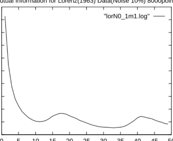
We take parameter settings r = 45.92, b = 4.0 and s = 16.0 [5], and use 25,000 x-ordinate points derived from a Runge-Kutta integrator with time step 0.01. A large amount of uniform noise was then added to the data, noise at ±10%. The mutual information analysis suggests a sampling rate of every 13 point.
0 10 20 30 40 50 60 70 80 90 100 0 5 10 15 20 25 30 35 40 45 50 Mutual Information Time Delay
Mutual Information for Lorenz(1963) Data(Noise 10%) 8000points "lorN0_1m1.log"
Figure: Mutual Information of Lorenz Data
A data set consisting of 1923 points remains and both a nearest neighbour analysis and a singular was undertaken, with results given in Table 1 and 2. This result suggests that an embedding of 4 or 5 should be sufficient to represent the attractor. This corresponds well with the theoretical upper bound of about 5, from the embedding theorem. The singular-value analysis shows the expected “noise floor” for eigenvalues 5 onwards suggesting that they are representing noise.
Embedding Dimension Percentage of False Nearest Neighbours 2 77% 3 3.3% 4 0.3% 5 0.3%
Table 1: The percentage of false nearest neighbours in the Lorenz data set
Eigenvector Eigenvalue 1 1534 2 74 3 3.7 4 0.64 5 0.59 6 0.59 7 0.57 8 0.56
Table 2: The eigenvalues of the sample covariance matrix with an embedding of 10 for the noisy lorenz dataset
We train a feedforward neural network with 120 hidden units, using conjugate gradient error minimisation. The embedding dimension, the size of the input layer, is increased from 2-unit to 10 units. The data is split into a training set of 1200 vectors and test set of 715 vectors. Each network configuration is trained 5 times with different random starting points, for 3000 epochs. The reported test set error is the mean minimum test set error reached in training. This point is normally found well before the training set error minimum is reached. Errors are calculated as relative errors [9], given by:
observation prediction observation observation t t t t t t −
(
)
−(
)
∑
∑
+ 2 1 2The denominator simply predicts the last observed value, which is the best that can be done for a random walk. A ratio above 1 is a worse than chance prediction.
0.05 0.08 0.11 0.14 0.17 0.2 0.23 0.26 2 3 4 5 6 7 8 9 10 Window Size Relative Error
Figure 4 The relative error of the predictor with varying window size for the noisy Lorenz data.. Averaged over 5 runs.
Figure 4 shows clearly a minimum prediction error with an embedding of 5, which corresponds well with both the theoretically expected embedding and that which is indicated by both the embedding heuristics. Moreover the increasing error for window sizes larger than 5 shows how the predictor can begin to model the noise in the system and thereby lose performance.
Tree Ring Data
This data set consists of 5405 data points recording tree ring data (measuring annual growth) at Campito mountain from 3435BC to 1969AD, [7]. The mutual information analysis of the data suggested a sampling rate of 1. There are no well established minimum in the graph, implying that every point is independent.
2 2.5 3 3.5 4 4.5 5 5.5 6 6.5 0 5 10 15 20 25 30 35 40 45 50 Mutual Information Time Delay
Mutual Information for Campito Tree Rings Data 5400 points "trings2.log"
The subsequent false nearest neighbour analysis and singular-value analysis are shown in Tables 3 and 4. The results here are not as clear as with the Lorenz data. The false nearest neighbour method suggests and embedding of 5, but the singular-value analysis does not give any strong indication of a suitable embedding dimension Embedding Dimension Percentage of False Nearest Neighbours 1 100% 2 13.6% 3 69.19% 4 1.6% 5 0.8%
Table 3: The percentage of false nearest neighbours in the Tree Ring data set.
Eigenvector Eigenvalue 1 1209 2 208 3 126 4 92 5 79 6 65 7 55
8 52
9 50
10 45
11 39
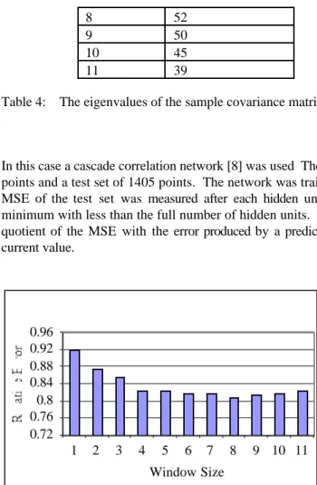
Table 4: The eigenvalues of the sample covariance matrix with an embedding of 16 for the tree ring data.
In this case a cascade correlation network [8] was used The data was split into two: a training set, of 4000 points and a test set of 1405 points. The network was trained with a maximum of 25 hidden units, and the MSE of the test set was measured after each hidden unit recruitment. In all cases this error was at a minimum with less than the full number of hidden units. The relative error was calculated as by taking the quotient of the MSE with the error produced by a predictor that always chooses the next value to be the current value. 0.72 0.76 0.8 0.84 0.88 0.92 0.96 1 2 3 4 5 6 7 8 9 10 11 Window Size
Figure 6: The relative error for the tree ring data test set, for varying window sizes and a trained cascade correlation network
From figure 6 it can be seen that the error falls to a minimum with a window of size 8 and then increases a little. The results show some correspondence with the nearest neighbour results and also the rising error is again indicative of a window size becoming too large. It is also noteworthy that the quality of the
predictions here is significantly worse than for the Lorenz data.
4 CONCLUSIONS
The results suggest that the embedding theorem and the false nearest neighbour method can provide useful heuristics for use in the design of neural networks for time series prediction. With two of the data sets examined here, the predicted embedding size corresponded with a network configuration that performed well, with economical resources. With our data sets we did not observe an overlarge embedding size to have a deleterious effect on the network. The tree ring data, however, showed that conclusions must be treated with caution, since poor predictive results were produced whatever the window size.
References
[1] Edwards, T., Tansley, D, S. W., Davey, N., Frank, R. J.(1997). Traffic Trends Analysis using Neural Networks. Proceedings of the International Workshop on Applications of Neural Networks to
[2] Patterson D W, Chan K H, Tan C M. 1993, Time Series Forecasting with neural nets: a comparative study. Proc. the international conference on neural network applictions to signal processing. NNASP 1993 Singapore pp 269-274.
[3] Bengio, S., Fessant F., Collobert D. A Connectionist System for Medium-Term Horizon Time Series Prediction. In Proc. Intl. Workshop Application Neural Networks to Telecoms pp308-315, 1995. [4] Dorffner, G. 1996, Neural Networks for Time Series Processing. Neural Network World 4/96,
447-468.
[5] Ababarnel H., D., I., Brown R., Sidorowich J., L. and Tsimring L., S., 1993, The analysis of observed chaotic data in physical systems. Reviews of Modern Physics, Vol. 65, No. 4 pp1331-1392 [6] Edwards, T., Tansley, D, S. W., Davey, N., Frank, R. J.(1997) Traffic Trends Analysis using Neural
Networks. Proceedings of the International Workshop on Applications of Neural Networks to Telecommuncations 3. pp. 157-164
[7] Fritts, H.C. et al. 1971. Multivariate techniques for specifying tree-growth and climatic relationships and for reconstructing anomalies in Paleoclimate. Journal of Applied Meteorology, 10, pp.845-864. [8] Fahlman, S.E. and C. Lebiere 1990. The Cascade-Correlation Learning Architecture. In Advances in
Neural Information Processing Systems 2 (D. S. Touretsky, ed.) pp 524-532. San Mateo, CA: Morgan Kaufmann.
[9] Gershenfeld N. A. and A. S. Weigend, The Future of Time Series. In Time Series Prediction: Forecasting the Future and Understanding the Past, Gershenfeld A. N.. and A. S. Weigen, eds, pp 1-70. 1993.