B-Alert with AcqKnowledge Quick Guide
Baseline Acquisition and Cognitive States Analysis
42 Aero Camino, Goleta, CA 93117 Tel (805) 685-0066 | Fax (805) 685-0067
Table
of
Contents
Introduction
... 2
What is B‐Alert?
... 2
Minimum System Requirements
... 3
Chapter
1:
Configuration
... 4
A.
Items Required for Use
... 4
B.
Connect Hardware and Check Impedance
... 4
Chapter
2:
B
‐
Alert
Gauges
GUI
... 6
Gauges Window
... 6
Chapter
3:
Acquiring
Baselines
for
B
‐
Alert
Classifications
... 7
A.
Baseline Acquisition with Alertness and Memory Profiler (AMP)
... 7
B.
Steps for AMP Baseline Acquisition
... 7
C.
Completing the AMP tasks
... 9
Chapter
4:
Acquisition
Troubleshooting
... 11
B‐Alert Baseline Issues
... 11
Appendix:
Data
Outputs
Guide
... 13
Overview
... 13
Classifying Cognitive States (B‐Alert And Workload Models):
... 14
Real‐Time Data Outputs Overview Table
... 16
Offline Data Outputs Overview Table
... 17
Classification (B‐Alert and Workload) Output
... 18
_Classification.csv
... 18
Power Spectral Densities Outputs
... 18
Diff_Class.csv
... 18
Diff_Raw.csv
... 20
Ref_Class.csv
... 21
Ref_Raw.csv
... 22
Heart Rate Outputs... 23
_HR_beat.csv
... 24
HR_epoch.csv
... 24
Z‐Score Outputs
... 24
_
ZScore_PSD.csv
... 26
Artifact
... 26
_missed_blocks.csv
... 26
Create
.def
File
Output
Files
... 27
Definition File (xxxx_ M7003500_A1.def)
... 27
BaselineReport.csv
... 27
Introduction
Welcome to the B-Alert® with AcqKnowledge Quick Guide. The purpose of this manual is to familiarize
AcqKnowledge users with the optionally licensed B-Alert® wireless EEG Cognitive States Analysis software, as well
as the various screens and file formats generated during an EEG study subject’s Baseline Definition file session.
What
is
B
‐
Alert?
B-Alert is a is a Bluetooth wireless system and sensor headset integrated with AcqKnowledge softwareto record up to 9 channels of monopolar EEG, plus one optional channel of ECG data. B-Alert Cognitive States Analysis software can be additionally used to create a “Baseline” file of a subject’s EEG profile by administering some simple onscreen tests, and storing this session data as a permanent reference for future EEG recordings. The B-Alert Brain State Gauges can be used to display a real-time view of B-Alert headset data as it is being acquired. The EEG data itself is recorded in AcqKnowledge via the wireless B-Alert hardware.
Although the B-Alert Cognitive States Analysis software covered in this manual is a stand-alone application manufactured by Advance Brain Monitoring Inc®, the following B-Alert features are fully accessible via the
AcqKnowledge application’s hardware* menu:
B-Alert Headset Check Impedance
B-Alert Headset AMP Baseline
B-Alert Show Brain State Gauges
Use B-Alert Definition File
The software controls for these features (as well as EEG analog and calculation channel setups) are initially explained in the Biopac AcqKnowledge Software Guide, and this manual is intended as an adjunct to assist the user in greater detail. Using B-Alert with AcqKnowledge should be easy and intuitive for users already familiar with AcqKnowledge. For specific information on using proprietary B-Alert software independently of AcqKnowledge, see the B-Alert Software Manual.
*In B-Alert hardware mode, the B-Alert menu replaces the MP menu.
For a full explanation of the B-Alert wireless EEG hardware and hardware setup, please refer to the B-Alert® X10 User Manual.
For step-by-step direction, request B-Alert X10 User Training Videos from [email protected].
Minimum
System
Requirements
Personal computer (PC) with minimum PentiumTM 2.4 GHz processor;
Minimum of 1 GB of installed RAM memory and 4 MB virtual memory;
Windows XP or Windows 7 operating system;
.NET framework version 3.5 installed;
Minimum of 50 MB hard disk space per 5-hour session;
One CD-ROM drive;
VGA or higher resolution video adapter;
One available USB port;
Chapter
1:
Configuration
A.
Items
Required
for
Use
B.
Connect
Hardware
and
Check
Impedance
Before starting Check Impedance, plug the B-alert USB Receiver into the PC and turn the headset to ON. Wait for the solid green LED pattern on both headset and B-Alert USB Receiver to confirm the Receiver and Headset have
connected. (Refer to the B-Alert X10 User Manual for full details on attaching the Headset to the subject).
The Check Impedance function allows the technician to test the impedance levels at each electrode site. Impedances measure resistance between the scalp and electrode in kΩ, where lower values reflect lower resistance and better conductivity between scalp and electrodes. In orderto optimize data quality, the manufacturer strongly recommends conducting an impedance check before starting any data collection.
In Acq
Knowledge
software
a
ccess Check Impedance via:1. B-Alert menu > B-Alert Headset Check Impedance
2. Click “Start Check Impedance” to perform the test.
B‐Alert Headset x10
Impedance values lower than 40kΩ will be highlighted in green.
Impedance values between 40kΩ and 80kΩ will be highlighted in yellow.
Impedance values higher than 80kΩ will be highlighted in red, indicating that the sensor is outside of the acceptable range.
Impedances generally will decrease for the first 30-45 minutes following application to a participant. For additional tips on lowering impedance values, refer to troubleshooting (pg.11). The manufacturer recommends getting all electrode sensors below 40kΩ for optimal data quality. Users are recommended to set a standard impedance threshold for data collections to maintain data quality across subjects. Having impedances higher than 40kΩ (yellow) will still collect good quality EEG and may not be reason to exclude a participant from continuing to collect, however, the manufacturer recommends getting impedances lower than 40kΩ for all 9 EEG sites and the Ref (mastoid sensors) sites before starting an acquisition. If high impedances are seen across ALL 9 EEG channels, try replacing the mastoid sensors before troubleshooting each EEG site -- high Reference impedance will impact ALL EEG impedance measurements.
The following output files are generated during an impedance test, thee files are useful for technical support not for data analysis:
xxxxxxxxx.ebsimpedance checking.csv: This CSV file will contain the impedance values from each impedance
test performed. If repeated impedance tests are performed for the subject, all of the values will be saved to the same CSV file, organized by system time.
xxxxxxxxx.ebsimpedance_checking_0_35_12.ebs: An impedance EBS file is saved in the subject folder for
each impedance test performed. The system time is included in the file name to allow simple file tracking.
Chapter
2:
B
‐
Alert
Gauges
GUI
In Acq
Knowledge
software
a
ccess the B-Alert Brain State Gauges via: B-Alert menu > Show Brain State GaugesGauges
Window
The gauges are fully customizable to optimize information display to fit the requirements of the user. The easy-to-read gauge and time series windows present second by second B-Alert classification metrics: Engagement, Workload, Drowsiness, and Heart Rate. Heat maps display EEG power spectral densities (PSD) in both spatial and temporal maps for the traditional Hz bands (Beta, Alpha, Theta, Sigma).
1. Gauges Meter Gauges: B‐Alert classifications averaged on a 3‐ second window, default to show Workload, High Engagement, Distraction, and Heart Rate
1
4
3
3. Heat Map Heat Map Gauges:4‐sec. averaged distribution of power spectra intensity across scalp
2
4. PSD
Surface Map Gauges:
Shows Average PSD
across all 9 channels
across time, with PSD
bin on x‐axis and
time on y‐axis. Theta – 3 ‐ 7 Hz Alpha – 8 ‐ 12 Hz Beta – 13 ‐ 29 Hz Sigma – 30 ‐40 Hz 2. Time Series Time Series Gauges ‐ second by second EEG Data in 15 second windows (Displays B‐Alert classification, PSD, and HR data)
5
5. Z‐Score
Z‐Score Histogram: displays second by second Z‐
Scored values ‐‐Default set to Alpha (8‐12Hz),
Theta (3‐7 Hz), and Heart Rate (Second by
Chapter
3:
Acquiring
Baselines
for
B
‐
Alert
Classifications
A.
Baseline
Acquisition
with
Alertness
and
Memory
Profiler
(AMP)
The acquisition of baseline data is used to create the individualized EEG profiles required for the B-Alert cognitive state metrics (B-Alert model and Workload models). The “Baseline” AMP obtains 5 minutes each of a 3-choice psychomotor vigilance task (3CVT), eyes open (EO), and eyes closed (EC). The “Drowsy” AMP extends the 3CVT to 20-minutes, which allows users to profile individuals unable to remain within a normal performance range during the 3CVT task, a predictor that may result in abnormal B-Alert classifications. Typically baseline data only needs to be obtained one time for each individual, if performed on a healthy, rested subject. However additional session iterations are recommended when pre- and post-conditional changes are made.
Baseline = ~ 15 minutes Drowsy = ~ 30 minutes Baseline configuration
15m_Baseline.apr
30m_Drowsy.apr
Task 1
3C‐VT (~7 min)
3C‐VT (~20 min)
Task 2
EO (~6 min)
EO (~6 min)
Task 3
EC (~6 min)
EC (~6 min)
Total Run Time
~19min
~32min
In Acq
Knowledge
software
access B-Alert Headset AMP Baseline feature via: 1. B-Alert menu > B-Alert Headset AMP Baseline2. Enter the Subject id (four digits), Group id (one digit) and Iteration number (one digit).
3. Select the desired baseline recording length (APR Setting). 4. Click OK in the AMP Baseline dialog.
The AMP (Alertness Memory Profiler) Baseline blue startup screen (shown on page 8, Fig. 3.1) will appear. Refer to pages 8-10 for full details about performing AMP Baseline tasks.
B.
Steps
for
AMP
Baseline
Acquisition
1.
Starting
AMP
acquisition
After a quality check is performed, an impedance check will be initiated. The following window (Fig. 3.1) will be shown; press the left arrow button on the keyboard to begin the impedance check.
Fig.
3.1
During the Impedance Check the following window will be shown (Fig. 3.2). Channels highlighted in green have passed the impedance check. Channels highlighted in red "fail" the impedance check, as the selected sensor site is too high. If any impedance values are high, the window indicating that sensors need to be adjusted will appear (Fig. 3.2). Click F11 to exit from this screen and return to the impedance check window. Click the ALL button to repeat the impedance test or click OK to continue to the AMP session. After the impedance check, the subject is ready to begin (Fig. 3.3).
It is important to note:All impedance values should have passing results before the AMP is started. Refer to the hardware manual or strip labeling for the electrode site naming convention. If impedance values have been previously checked using the B-Alert > Check Impedance menu item, you may choose to bypass this built-in impedance check by pressing OK at any time.
Fig.
3.2
Fig.
3.3
C.
Completing
the
AMP
tasks
The subject will be prompted to complete at least three neurocognitive tests. The standard session length for eyes open and eyes closed is 5-minutes, with additional time extended if the user fails to respond consistently (suggesting they fell asleep, thereby distorting the baseline measures).
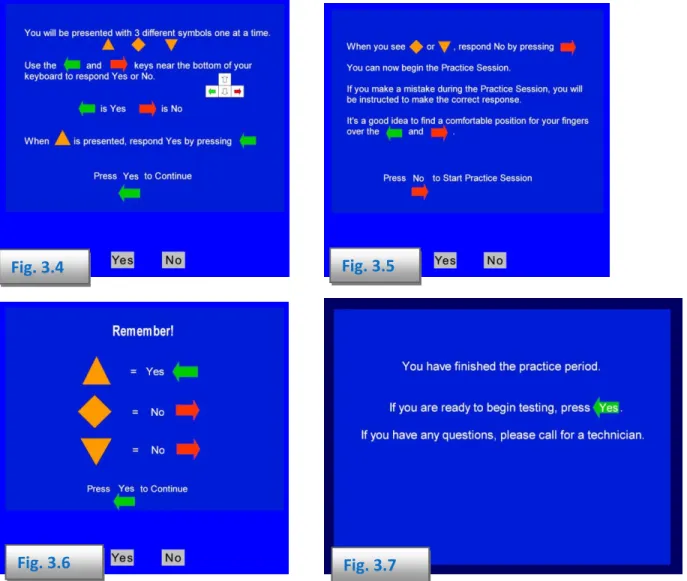
a. Three-Choice Vigilance Task (3CVT)
After the instructions are presented (Figures 3.4 and 3.5), the 3CVT session begins with a Practice Session. During the practice session, AMP will alert the subject when an incorrect response is made (Figure 3.6) to insure that he/she understands the task. As soon as the user demonstrates that they understand each of the responses, the practice session will terminate (Fig 3.7) and the testing session will begin.
Fig.
3.5
Fig.
3.4
Fig.
3.6
Fig.
3.7
The length of the 3CVT (after the practice period) will either be 5- or 20-minutes long, depending on the baseline type selected. During the first 5-minute period, stimuli appear frequently and require a high state of alertness. The inter-stimulus intervals are extended in the remaining 15 minutes of the 3CVT in order to better identify individuals who are unable to remain engaged (i.e., excessive daytime drowsiness or other sleep related disorders). Subjects who are unable to sustain performance within a normal range across the 3CVT will be flagged as having an invalid baseline session.
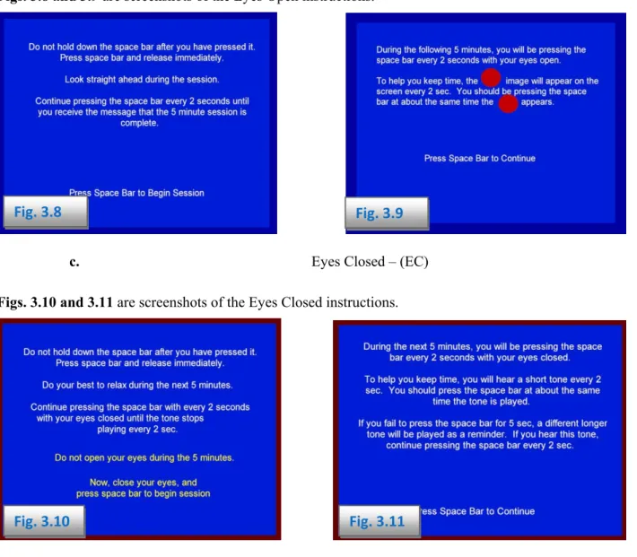
b. Eyes Open – (EO) Figs. 3.8 and 3.9 are screenshots of the Eyes Open instructions.
Fig.
3.8
Fig.
3.9
c. Eyes Closed – (EC)
Figs. 3.10 and 3.11 are screenshots of the Eyes Closed instructions.
Fig.
3.10
Fig.
3.11
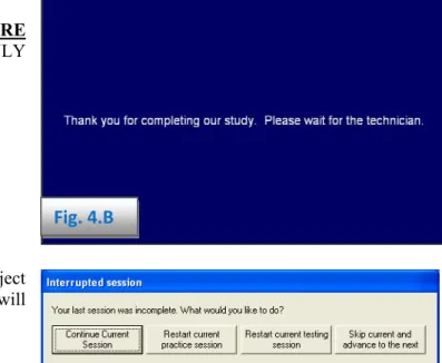
After completing the AMP, a completion dialogue will appear (Fig. 3.12). Once acquired, the AMP session files will be stored in the subject’s folder. The definition file needed for B-Alert classifications will also be automatically generated and placed in the subject’s folder. The .def file is required for generating EEG classification metrics in Real-Time during acquisition or during offline data analysis.
Chapter
4:
Acquisition
Troubleshooting
B‐Alert Baseline Issues
During any of the three tasks in B-Alert Baseline, the technician may interrupt the session using three key controls:
F3, F8, and F11.
Fig.
4.B
F3 - takes the subject to the very end of the ENTIRE
AMP SESSION and is available for use ONLY during the instruction windows (Fig.4.B).
F8 - allows the technician to interrupt the subject
ONLY during Testing Sessions. This window will then appear:
At this point, the technician can choose the appropriate action. If the technician chooses the option to restart the current testing session, the following window will then appear:
Fig. 4.A.1
In order to recollect data, the technician must make note of any problems that occurred during the testing, i.e., drowsiness, low batteries, EEG, etc. Select Other, if none of displayed problems are appropriate. (Fig.4.A.1)
The following three windows are examples of when to use this button:
Fig.
4.A.2
Fig.
4.A.3
When F8 is pressed during Figs. 4.A.2 and 4.A.3, the interrupted session window prompts the technician to continue, restart or skip the current testing session. If restarting the current testing session, the repeated session info window will appear. For data quality maintenance, it is important to best describe the problems that occurred while testing.
Upon completing the AMP session, Fig. 4.A.3 will appear. Once the technician exits out of this screen using F11, the main screen of BAA will appear on the subject’s computer with the AMP ABD Checking window shown.
The AMP ABD Checking window displays the processing of the .def and report output files. “Definition File is created” pop up window will notify user when processing is complete (5-10 min).
Appendix:
Data
Outputs
Guide
Overview
B-Alert software allows users to utilize Artifact Identification, EEG-Classification, PSD, and ECG algorithms if desired. These data outputs are either created in real time (See Real Time Data Outputs) or offline (see Create .def file Outputs and Generate Reports Outputs). Below is an overview of some of the methods and techniques used by B-Alert to compute its various measures.
Computing Power Spectral Densities: Power spectral density (PSD) is computed by performing Fast Fourier Transform (FFT) on a segment of data that is of interest, and calculating the amplitudes of the sinusoidal components for designated frequency bins. Input variables to this transformation are an EEG segment for which PSD is to be computed, and its length; output variables include PSD amplitudes. Frequency domain variables are based on the power spectral density derived after application of a 50% overlapping window, and a FFT with ('_raw') and without ('_class') application of a Kaiser window. The B-Alert software provides two sets of PSD values (Ref_Raw and Ref-Class) from 1 to 40 Hz for each EEG channel that are logged to obtain a Gaussian distribution. Selected 1-Hz bins are averaged, then logged to create conventional EEG bands (e.g., theta = 3 – 7 Hz, alpha = 8 – 12 Hz, etc.). 'Diff_' files contain data for Differential EEG channels used for B-Alert’s's Classification measures (FzPOz, CzPO, FzC3, C3C4, F3Cz). 'Ref_' files contain PSD values for 9 referential EEG channels (POz, Fz, Cz, C3, C4, F3, F4, P3, P4).
Both sets of PSD output files apply a 50% overlapping window which averages the PSD across three x one-second overlays to smooth the data. The illustration below shows that overlays 0, 1 and 2 are averaged (each overlay
containing 256 data points with 128 data points being shared for each overlay) to provide the PSD values for epoch n. 50% Overlap – Ref_Raw, Diff_Raw 50% Overlap – Ref_Class, Diff_Class
(Kaiser windowing applied)
For the 'Ref_Class.csv' and 'Diff_Class.csv' PSD calculation, a Kaiser window is applied to each overlay in order to accentuate the contribution of power from the signal in the middle third of the overlay and minimize the impact of signal near each edge of the overlay. Windowing reduces the likelihood of extreme PSD values resulting from edge-effects when an EEG wave shape does not begin or end at the exact edge of an overlay. No Kaiser windowing is used for Ref_Raw and Diff_Raw analysis. The manufacturer recommends using the _Raw data for users wishing to use PSD based computations using this PSD overlaying procedure.
Decontaminating Signals: Prior to computing the 1-Hz PSD bins, the raw signals are processed to eliminate known artifacts. Spikes, excursions and amplifier saturations, which occur when ambulatory EEG is acquired, can impact both low and high frequencies. EMG will contaminate the beta and sigma frequency ranges. Eye blinks occur in the same frequency range as theta activity.
Before Decontamination:
After Decontamination:
Epoch n Overlay 0 Overlay 1 Overlay 2 Epoch n 1 0 2 Excursions and amplifier saturation – contaminated periods are replaced with zero values starting and ending nal value is interpolated.
y, the overlay is not included in the each overlay) and Low
ng two overlays. If
ks –wavelet transforms deconstruct the signal and a regression equation is used to identify
Workload
Models)
at zero crossing before and after each event. Spikes caused by artifact are identified and sig
Invalid Epochs -- If more than 128 zero values are inserted for an overla
epoch average, if two of the three overlays are rejected, the epoch is classified as ‘invalid’ (-99999 inserted for PSD value) and should be excluded from analysis.
EMG -- a combination of High Frequency EMG (based off 70 - 128 Hz bins for
Frequency EMG (based off 35 – 40 Hz) is used to identify periods with excessive EMG. If only one overlay has EMG the PSD for the epoch is based on the average of the remaini
excessive EMG is detected in two overlays, the second is classified as ‘EMG’ and should be excluded from analysis.
Eye Blin
the EEG regions contaminated with eye blinks. Representative EEG preceding the eye blink is
inserted in the contaminated region.
Classifying
Cognitive
States
(B
‐
Alert
And
:
B-Alert Wireless EEG bio-metrics are normalized to an individual subject using 5-7 minutes of baseline data from s
-ECT THESE 3 SPECIFIC TA FOR EACH PARTICIPANT WILL RESULT IN AN
three distinct tasks (3-Choice Vigilance, Eyes Open, and Eyes Closed) with the sleep onset class predicted from the baseline PSD values; for a total of 15-17 min of data across tasks. Based on this identification data, a probability-of-fit is then generated for each of the four classes for each epoch with the sum of the probabilities across the four classe equaling 1.0 (e.g., 0.45 high engagement, 0.30 low engagement, 0.20 distraction and 0.05 sleep onset). Cognitive State for a given second represents the class with the greatest probability using numeric labels (.1= sleep onset, .3= distraction, .6= low engagement, and .9= high engagement). B-Alert cognitive state metrics are derived for each one second epoch using 1 Hz power spectra densities (PSD) (from the bins from differential sites FzPOz, CzPO, FzC3, C3C4, F3Cz) in a four-class quadratic discriminant function analysis (DFA) that is fitted to the individual’s unique EEG patterns. The table below identifies and briefly describes each baseline task, and associates the task with the B-Alert classification.
******FAILURE TO COLL SKS
Baseline
task
Action
B
‐
Alert
Class
probabilities
3‐choice vigilance task
(~7‐min; optional 20‐
min)
Discriminate between primary vs. secondary or
tertiary stimulus every 1.5 to 3‐seconds
High Engagement
Eyes open (5‐min)
Respond to visual probe every 2‐seconds
Low Engagement
Eyes closed (5‐min)
Respond to audio tone every 2‐seconds Distraction
None
Derived by regression from other three tasks
Sleep Onset
The B-Alert probabilities for each individual should be interpreted in a relative, rather than absolute manner. Three standardized baseline tasks normalize the cognitive state metrics to each individual. High population variability for EEG activity requires individualized model fitting, which is done for each 1-Hz bin (from 1-40Hz), and is not fit to classic summed bandwidths/rhythms (i.e. theta, alpha, beta, etc.) to optimize classification measures.
Two individuals will generate somewhat different probabilities for the same task due to a) their innate capability, and b) their state during acquisition of baseline data. If a participant is mentally balancing their checkbook during the eyes closed task, for example, they will not generate as much alpha activity as they would in a relaxed state. This may increase the occurrence of Distraction probabilities when applied to a different task in which they do mentally relax. Participants are more aroused the first time they complete a baseline session due to the novelty, so it is preferable to reuse the individual’s DFA to classify new data/sessions rather than re-run the identification tasks repeatedly.
Participants should avoid consumption of caffeine or nicotine immediately prior to baseline/identification acquisition; and the session should occur in the morning (8am-10am) after a full night of sleep to collect an optimal session. The B-Alert Workload metric is a generalized model (i.e., it is not individually fit), thus it should also be interpreted in a relative manner. For the linear 2-class workload DFA, probabilities closer to 1 reflect higher workload. EEG workload is correlated with increased working memory load and difficulty level in mental arithmetic and other complex problem solving tasks. B-Alert has 2 workload models -- one model was built on a Forward digit span (FBDS) task (recommended to use -- fits for 85% of population) and the other built on a backward digit span (BDS) task (fits 15% of population). B-Alert's data outputs also contain the mean probability between the FBDS and BDS model.
Z-scoring is a useful transformation to convert the relative B-Alert metrics into values that can be compared across participants, or for a repeated-measures within-subject experimental design.
Output files: The output files generated with the B-Alert software share common formatting features. For example, all file names begin with the nine digit subject/session number (XXXXXXXXX), followed by the label which describes the data. For generated files, one row of data is provided per second of recording time. The first column lists the subject/session number, the second column the elapsed time (since the start of recording) in
hour::minute:second:millisecond (HH:MM:SS:MS), and the third column the system clock time associated with the start of the primary (middle) overlay for the epoch. Output files use a comma separated value (CSV) format for easy import into statistical/analytical software applications.
Real
‐
Time
Data
Outputs
Overview
Table
Real‐Time Output file name
Description
Data
file
Xxxxxxxxx.ebs
European data format containing nine raw and nine
decontaminated EEG channels, raw ECG channel, plus derived
heart rate, head movement value and head movement level
Xxxxxxxxx_Impedance.csv
Lists the values obtained for each channel each time impedance
was measured
Automatically
Generated
during
Acquisition
–
for
all
EEG
Channels
Xxxxxxxxx_Ref_Raw.csv
Absolute PSD from 1 to 40 Hz, relative PSD from 1 to 40 Hz, and
EEG bands labeled by channel (no edge‐effect window)
Xxxxxxxxx_Ref_Class.csv
Absolute PSD from 1 to 40 Hz, relative PSD from 1 to 40 Hz, and
EEG bands labeled by channel (with Kaiser window)
Automatically
Generated
during
Acquisition
–
Derived
Signals
Xxxxxxxxx_HR_beat.csv
Presentation of heart rate based on beat‐to‐beat interval
Xxxxxxxxx_HR_epoch.csv
Beat‐to‐beat heart rate interpolated to sec‐by sec value
Optionally
Generated
with
B
‐
alert
Cognitive
State
Classifications
Xxxxxxxxx_Classification.csv
Probabilities for sleep, distraction, low and high engagement,
cognitive state from DFA with greatest probability, probability of
high workload based on forward and backward digit span (FBDS),
backward digit span (BDS), and average of FBDS and BDS
Xxxxxxxxx_Diff_Raw.csv
Absolute PSD from 1 to 40 Hz, relative PSD from 1 to 40 Hz, and
EEG bands for differential channels: FzPO,CzPO,FzC3,C3C4, and
F3Cz (no edge‐effect window)
Xxxxxxxxx_Diff_Class.csv
Absolute PSD from 1 to 40 Hz, relative PSD from 1 to 40 Hz, and
EEG bands for 5 differential channels FzPOz, CzPO, FzC3, C3C4,
F3Cz (with Kaiser window)
Xxxxxxxxx_Zscore_class.csv
Updates and applies mean and standard deviation with each new
second to provide z‐scores for B‐Alert cognitive states (sleep
onset, distraction, low and high engagement, three workload
measures)
Xxxxxxxxx_Zscore_psd.csv
Updates and applies mean and standard deviation with each new
second to provide z‐scores for PSD for all channels requested in
initialization process
Offline
Data
Outputs
Overview
Table
Real‐Time Output file Extensions
Description
EEG
Classification
Reports
.eec
Lists the values obtained for each channel each time impedance
was measured.
_datasummary.csv
Summary EEG classification information averaged across an
entire session.
Heart
Rate
Reports
HR.csv
S
econd by Second (Epoch‐by‐epoch) heart rate data.Summary_HR.csv
Summary heart rate data over the entire session.
HRV.csv
Heart Rate Variability data averaged over each 5‐minute window
in the session.
PSD_HRV.csv
Contains the ECG (EKG) Power Spectral densities for each 5min
interval from .01‐.40Hz.
Power
Spectral
Density
(PSD)
Reports
_Ref:
Referential
EEG
channels
(F3,Fz,F4,C3,Cz,C4,P3,PO,P4)
_Class:
Differential
EEG
channels
(FzPO, CzPO, FzC3, C3C4, F3Cz)
.psd
Second to second PSDs are computed for each channel (relative
and absolute PSD) for 3‐40Hz bin, and PSD bandwidths Theta
(Fast, Slow, and Total), Alpha (Fast, Slow, and Total), Beta,
Gamma, Sigma.
.sbw
Summary Bandwidth information for Theta, Alpha, Beta, Gamma,
and Sigma across the entire session: Theta (Fast, Slow, and Total),
Alpha (Fast, Slow, and Total), Beta, Gamma, Sigma.
.EBW
Second to Second PSD Bandwidth data for Theta (Fast, Slow, and
Total), Alpha (Fast, Slow, and Total), Beta, Gamma, Sigma.
Obsolete
Output
Files
.wf10
.df10
.fpc
These File types are Obsolete and no longer supported.
During an Acquisition (and in Real-Time playback mode), the B-alert Software will generate the following data outputs:
XXXXXXXX _Classification.csv (if B-Alert or Workload checked and .def selected prior to start) XXXXXXXX_Diff_Class.csv XXXXXXXX _Diff_Raw.csv XXXXXXXX _HR_beat.csv XXXXXXXX _HR_epoch.csv XXXXXXXX _Ref_Class.csv XXXXXXXX _Ref_Raw.csv
Classification
(B
‐
Alert
and
Workload)
Output
_Classification.csv
Classification.csv shows the second by second (epoch by epoch) data outputs for two EEG models: 4-Class B-Alert model of drowsiness: (Sleep Onset, Distraction, Low Engagement, High Engagement) and 2-Class model of
Workload (High Workload) These outputs will ONLY be generated if the user has checked either of the 'Brain State' check boxes (B-Alert Classification and Workload Classification) and selected the appropriate .def file prior to initializing a data Acquisition.
Column
Column
Name
Description
A
SessionNum
Session Name (.ebs File Name)
B
Elapsed Time
Total Elapsed Time for session in seconds (hh:mm:ss:ms)
C
Clock Time
Local Computer Time
(hh:mm:ss:ms)
D
ProbSleepOnset
Sleep Onset classification probability (0‐1)
E
ProbDistraction
Distraction classification Probability (0‐1)
F
ProbLowEng
Low Engagement classification probability (0‐1)
G
ProbHighEng
High Engagement classification probability (0‐1)
H
CogState
The highest Probability in columns D,E,F,G will determine what the
epoch is classified. Classifications are: .1: Sleep onset, .3: Distraction, .6:
Low Engagement, .9: High Engagement
Seconds with excessive artifact where classification data could not be
computed are identified with .05, 1 and 2
I
ProbFBDSWorkload
Raw Workload probability (FBDS model), where higher probability
reflects higher WL (FBDS is the best model for 85% of population)
J
ProbBDSWorkload
Alternate WL model (BDS model): Not recommended for use, higher
probability reflects higher WL (Best WL model for other 15% of
population)
K
ProbAveWorkload
Average Workload between 2 models (in Columns I and J)
Power
Spectral
Densities
Outputs
_
Diff_Class.csv_Diff_Raw.csv _Ref_Class.csv
_Ref_Raw.csv
Power spectral density (PSD) is computed by performing Fast Fourier Transform (FFT) on a segment of data that is of interest, and calculating the amplitudes of the sinusoidal components for designated frequency bins. Input variables to this transformation are an EEG segment for which PSD is to be computed, and its length; output variables include PSD amplitudes. Frequency domain variables are based on the power spectral density derived after application of a 50% overlapping window, and a FFT with (_raw) and without (_class) application of a Kaiser window. Refer to Outputs Overview above for additional information regarding the PSD analysis procedures.
Diff_Class.csv
PSDs (1-40Hz) for the differential channels (FzPOz, CzPO, FzC3, C3C4, F3Cz) are computed for generating B-Alert’s's classifications for each second of a given .ebs file. PSDs in this file are computed for each second of a given session with the Kaiser Windowing procedure described above. Relative power values are derived by subtracting the
Column Column Name Description
A SessionNum Session Name (.ebs File Name)
B Elapsed Time Total Elapsed Time for session in seconds (hh:mm:ss:ms)
C Clock Time Local Computer Time or ESU TimeStamp (if configured)
(hh:mm:ss:ms)
D fzpoz_1 PSD power at channel FzPoz (with Kaiser windowing) for the 1 Hz bin E fzpoz_2 PSD power at channel FzPoz (with Kaiser windowing) for the 2 Hz bin F ‐ AQ fzpoz_3‐40 PSD power at channel FzPoz (with Kaiser windowing) for the 3‐40 Hz
bins
AR fzpoz_rel1 Relative PSD power at channel FzPoz (with Kaiser windowing) for 1 Hz
Bin
AS ‐ CE fzpoz_rel2‐rel40 Relative PSD power at channel FzPoz (with Kaiser windowing) for 2‐40
Hz Bin
CF fzpoz_Delta_1_2 PSD for Delta Bandwidth at channel FzPoz (not relative PSD) summed
from Hz bins 1‐2
CG fzpoz_ThetaSlow_3_5 PSD for Theta‐Slow Bandwidth (not relative PSD) summed from Hz bins
3‐5
CH fzpoz_ThetaFast_5_7 PSD for Theta‐Fast Bandwidth (not relative PSD) summed from Hz bins
5‐7
CI fzpoz_ThetaTotal_3_7 PSD for Theta‐Total Bandwidth (not relative PSD) summed from Hz
bins 3‐7
CJ fzpoz_AlphaSlow_8_10 PSD for Alpha‐Slow Bandwidth (not relative PSD) summed from Hz bins
8‐10
CK fzpoz_AlphaFast_10_12 PSD for Alpha‐Fast Bandwidth (not relative PSD) summed from Hz bins
10‐12
CL fzpoz_AlphaTotal_8_12 PSD for Alpha‐Fast Bandwidth (not relative PSD) summed from Hz bins
8‐12
CM fzpoz_Beta_13_29 PSD for Beta Bandwidth (not relative PSD) summed from Hz bins 13‐29 CN fzpoz_Sigma_13_29 PSD for Sigma Bandwidth (not relative PSD) summed from Hz bins 13‐
29
CO czpoz_1 PSD power at channel CzPOz (with Kaiser windowing) for the 1 Hz bin
CP ‐ QF PSD/Relative PSD information for all differential channels (CzPOz,
FzC3, C3C4, F3Cz uses the same naming convention as fzpoz
(described above)
QG ThetaOverall_3_7 PSD Across ALL 5 differential channels (FzPoz, CzPoz, FzC3, C3C4, F3Cz)
for Theta‐Total Bandwidth (not relative PSD) summed from Hz bins 3‐7 QH AlphaOverall_8_12 PSD Across ALL 5 differential channels (FzPoz, CzPoz, FzC3, C3C4, F3Cz)
for Alpha Bandwidth (not relative PSD) summed from Hz bins 8‐12 QI BetaOverall_13_29 PSD Across ALL 5 differential channels (FzPoz, CzPoz, FzC3, C3C4, F3Cz)
for Beta Bandwidth (not relative PSD) summed from Hz bins 13‐29 QJ SigmaOverall_30_40 PSD Across ALL 5 differential channels (FzPoz, CzPoz, FzC3, C3C4, F3Cz)
for Beta Bandwidth (not relative PSD) summed from Hz bins 30‐40
Diff_Raw.csv
PSDs (1-40Hz) for the differential channels (FzPOz, CzPO, FzC3, C3C4, F3Cz) are computed for generating B-Alert’s's classifications for each second of a given .ebs file. PSDs in this file computed for each second of a given session without the Kaiser Windowing procedure. Relative power values are derived by subtracting the logged power
of the individual Hz bin from the summed logged power for the EEG band (1 – 40 Hz) for that channel.
Column
Column
Name
Description
A
SessionNum
Session Name (.ebs File Name)
B
Elapsed Time
Total Elapsed Time for session in seconds (hh:mm:ss:ms)
C
Clock Time
Local Computer Time or ESU TimeStamp (if configured)
(hh:mm:ss:ms)
D
fzpoz_1
PSD power at channel FzPoz (without Kaiser windowing) for the 1
Hz bin
E
fzpoz_2
PSD power at channel FzPoz (without Kaiser windowing) for the 2
Hz bin
F ‐ AQ
fzpoz_3‐40
PSD power at channel FzPoz (without Kaiser windowing) for the 3‐
40 Hz bins
AR
fzpoz_rel1
Relative PSD power at channel FzPoz (without Kaiser windowing)
for 1 Hz Bin
AS ‐ CE
fzpoz_rel2‐rel40
Relative PSD power at channel FzPoz (without Kaiser windowing)
for 2‐40 Hz Bin
CF
fzpoz_Delta_1_2
PSD for Delta Bandwidth at channel FzPoz (not relative PSD)
summed from Hz bins 1‐2 (without Kaiser windowing)
CG
fzpoz_ThetaSlow_3_5
PSD for Theta‐Slow Bandwidth (not relative PSD) summed from Hz
bins 3‐5 (without Kaiser windowing)
CH
fzpoz_ThetaFast_5_7
PSD for Theta‐Fast Bandwidth (not relative PSD) summed from Hz
bins 5‐7 (without Kaiser windowing)
CI
fzpoz_ThetaTotal_3_7
PSD for Theta‐Total Bandwidth (not relative PSD) summed from Hz
bins 3‐7(without Kaiser windowing)
CJ
fzpoz_AlphaSlow_8_10
PSD for Alpha‐Slow Bandwidth (not relative PSD) summed from Hz
bins 8‐10 (without Kaiser windowing)
CK
fzpoz_AlphaFast_10_12
PSD for Alpha‐Fast Bandwidth (not relative PSD) summed from Hz
bins 10‐12 (without Kaiser windowing)
CL
fzpoz_AlphaTotal_8_12
PSD for Alpha‐Fast Bandwidth (not relative PSD) summed from Hz
bins 8‐12(without Kaiser windowing)
CM
fzpoz_Beta_13_29
PSD for Beta Bandwidth (not relative PSD) summed from Hz bins
13‐29 (without Kaiser windowing)
CN
fzpoz_Sigma_13_29
PSD for Sigma Bandwidth (not relative PSD) summed from Hz bins
13‐29 (without Kaiser windowing)
CO
czpoz_1
PSD power at channel CzPOz (with Kaiser windowing) for the 1 Hz
bin (without Kaiser windowing)
CP ‐ QF
PSD/Relative PSD information for all differential channels (CzPoz,
FzC3, C3C4, F3Cz uses the same naming convention as fzpoz
(described above)
QG
ThetaOverall_3_7
PSD Across ALL 5 differential channels (FzPoz, CzPoz, FzC3, C3C4,
F3Cz) for Theta‐Total Bandwidth (not relative PSD) summed from
Hz bins 3‐7 (without Kaiser windowing)
QH
AlphaOverall_8_12
PSD Across ALL 5 differential channels (FzPoz, CzPoz, FzC3, C3C4,
8‐12 (without Kaiser windowing)
QI
BetaOverall_13_29
PSD Across ALL 5 differential channels (FzPoz, CzPoz, FzC3, C3C4,
F3Cz) for Beta Bandwidth (not relative PSD) summed from Hz bins
13‐29 (without Kaiser windowing)
QJ
SigmaOverall_30_40
PSD Across ALL 5 differential channels (FzPoz, CzPoz, FzC3, C3C4,
F3Cz) for Beta Bandwidth (not relative PSD) summed from Hz bins
30‐40 (without Kaiser windowing)
Ref_Class.csv
PSDs (1-40Hz) for the referential channels (POz, Fz, Cz, C3, C4, F3, F4, P3, P4) are computed for generating B-Alert's classifications for each second of a given .ebs file. PSDs in this file are computed for each second of a given session with the Kaiser Windowing procedure described above. Relative power values (_rel) are derived by
subtracting the logged power of the individual Hz bin from the summed logged power for the EEG band (1 – 40 Hz) for that channel.
Column
Column
Name
Description
A
SessionNum
Session Name (.ebs File Name)
B
Elapsed Time
Total Elapsed Time for session in seconds (hh:mm:ss:ms)
C
Clock Time
Local Computer Time or ESU TimeStamp (if configured)
(hh:mm:ss:ms)
D
POz_1
PSD power at channel POz (with Kaiser windowing) for the 1 Hz bin
E
POz_2
PSD power at channel POz (with Kaiser windowing) for the 2 Hz bin
F ‐ AQ
POz_3‐40
PSD power at channel POz (with Kaiser windowing) for the 3‐40 Hz
bins
AR
POz_rel1
Relative PSD power at channel POz (with Kaiser windowing) for 1
Hz Bin
AS ‐ CE
POz_rel2‐rel40
Relative PSD power at channel POz (with Kaiser windowing) for 2‐
40 Hz Bin
CF
POz_Delta_1_2
PSD for Delta Bandwidth at channel POz (not relative PSD) summed
from Hz bins 1‐2 (with Kaiser windowing)
CG
POz _ThetaSlow_3_5
PSD for Theta‐Slow Bandwidth at channel POz (not relative PSD)
summed from Hz bins 3‐5 (with Kaiser windowing)
CH
POz _ThetaFast_5_7
PSD for Theta‐Fast Bandwidth at channel POz (not relative PSD)
summed from Hz bins 5‐7 (with Kaiser windowing)
CI
POz _ThetaTotal_3_7
PSD for Theta‐Total Bandwidth at channel POz (not relative PSD)
summed from Hz bins 3‐7 (with Kaiser windowing)
CJ
POz _AlphaSlow_8_10
PSD for Alpha‐Slow Bandwidth at channel POz (not relative PSD)
summed from Hz bins 8‐10 (with Kaiser windowing)
CK
POz _AlphaFast_10_12
PSD for Alpha‐Fast Bandwidth at channel POz (not relative PSD)
summed from Hz bins 10‐12 (with Kaiser windowing)
CL
POz _AlphaTotal_8_12
PSD for Alpha‐Fast Bandwidth at channel POz (not relative PSD)
summed from Hz bins 8‐12 (with Kaiser windowing)
CM
POz _Beta_13_29
PSD for Beta Bandwidth at channel POz (not relative PSD) summed
from Hz bins 13‐29 (with Kaiser windowing)
CN
POz _Sigma_13_29
PSD for Sigma Bandwidth at channel POz (not relative PSD)
(described above‐‐ all with Kaiser windowing)
ADY
ThetaOverall_3_7
Mean PSD across ALL 9 referential channels (POz, Fz, Cz, C3, C4, F3,
F4, P3, P4) for Theta‐Total Bandwidth (not relative PSD) summed
from Hz bins 3‐7 (with Kaiser windowing)
ADZ
AlphaOverall_8_12
Mean PSD across ALL 9 referential channels (POz, Fz, Cz, C3, C4, F3,
F4, P3, P4) for Alpha Bandwidth (not relative PSD) summed from
Hz bins 8‐12 (with Kaiser windowing)
AEA
BetaOverall_13_29
Mean PSD across ALL 9 referential channels (POz, Fz, Cz, C3, C4, F3,
F4, P3, P4) for Beta Bandwidth (not relative PSD) summed from Hz
bins 13‐29 (with Kaiser windowing)
AEB
SigmaOverall_30_40
Mean PSD across ALL 9 referential channels (POz, Fz, Cz, C3, C4, F3,
F4, P3, P4) for Sigma Bandwidth (not relative PSD) summed from
Hz bins 30‐40 (with Kaiser windowing)
Ref_Raw.csv
PSDs (1-40Hz) for the referential channels (POz, Fz, Cz, C3, C4, F3, F4, P3, P4) are computed for generating B-Alert's classifications for each second of a given .ebs file. PSDs in this file are computed for each second of a given session without the Kaiser windowing procedure. Relative power values (_rel) are derived by subtracting the logged
power of the individual Hz bin from the summed logged power for the EEG band (1 – 40 Hz) for that channel.
Column
Column
Name
Description
A
SessionNum
Session Name (.ebs File Name)
B
Elapsed Time
Total Elapsed Time for session in seconds
(hh:mm:ss:ms)
C
Clock Time
Local Computer Time or ESU TimeStamp (if
configured)
(hh:mm:ss:ms)
D
POz_1
PSD power at channel POz (without Kaiser windowing)
for the 1 Hz bin
E
POz_2
PSD power at channel POz (without Kaiser windowing)
for the 2 Hz bin
F ‐ AQ
POz_3‐40
PSD power at channel POz (without Kaiser windowing)
for the 3‐40 Hz bins
AR
POz_rel1
Relative PSD power at channel POz (without Kaiser
windowing) for 1 Hz Bin
AS ‐ CE
POz_rel2‐rel40
Relative PSD power at channel POz (with Kaiser
windowing) for 2‐40 Hz Bin
CF
POz_Delta_1_2
PSD for Delta Bandwidth at channel POz (not relative
PSD) summed from Hz bins 1‐2 (without Kaiser
windowing)
CG
POz _ThetaSlow_3_5
PSD for Theta‐Slow Bandwidth at channel POz (not
relative PSD) summed from Hz bins 3‐5 (without
Kaiser windowing)
CH
POz _ThetaFast_5_7
PSD for Theta‐Fast Bandwidth at channel POz (not
relative PSD) summed from Hz bins 5‐7 (without
Kaiser windowing)
CI
POz _ThetaTotal_3_7
PSD for Theta‐Total Bandwidth at channel POz (not
relative PSD) summed from Hz bins 3‐7(without Kaiser
windowing)
CJ
POz _AlphaSlow_8_10
PSD for Alpha‐Slow Bandwidth at channel POz (not
Kaiser windowing)
CK
POz _AlphaFast_10_12
PSD for Alpha‐Fast Bandwidth at channel POz (not
relative PSD) summed from Hz bins 10‐12 (without
Kaiser windowing)
CL
POz _AlphaTotal_8_12
PSD for Alpha‐Fast Bandwidth at channel POz (not
relative PSD) summed from Hz bins 8‐12(without
Kaiser windowing)
CM
POz _Beta_13_29
PSD for Beta Bandwidth at channel POz (not relative
PSD) summed from Hz bins 13‐29 (without Kaiser
windowing)
CN
POz _Sigma_13_29
PSD for Sigma Bandwidth at channel POz (not relative
PSD) summed from Hz bins 13‐29 (without Kaiser
windowing)
CO
Fz_1
PSD power at channel Fz (without Kaiser windowing)
for the 1 Hz bin CP ‐
ADX
PSD/Relative PSD information for all referential
channels (POz, Fz, Cz, C3, C4, F3, F4, P3, P4) uses
same naming convention and analysis as Fz (described
above‐‐all without Kaiser windowing)
ADY
ThetaOverall_3_7
Mean PSD across ALL 9 referential channels (POz, Fz,
Cz, C3, C4, F3, F4, P3, P4) for Theta‐Total Bandwidth
(not relative PSD) summed from Hz bins 3‐7 (without
Kaiser windowing)
ADZ
AlphaOverall_8_12
Mean PSD across ALL 9 referential channels (POz, Fz,
Cz, C3, C4, F3, F4, P3, P4) for Alpha Bandwidth (not
relative PSD) summed from Hz bins 8‐12 (without
Kaiser windowing)
AEA
BetaOverall_13_29
Mean PSD across ALL 9 referential channels (POz, Fz,
Cz, C3, C4, F3, F4, P3, P4) for Beta Bandwidth (not
relative PSD) summed from Hz bins 13‐29 (without
Kaiser windowing)
AEB
SigmaOverall_30_40
Mean PSD across ALL 9 referential channels (POz, Fz,
Cz, C3, C4, F3, F4, P3, P4) for Sigma Bandwidth (not
relative PSD) summed from Hz bins 30‐40 (without
Kaiser windowing)
Heart Rate Outputs
_HR_beat.csv _HR_epoch.csv
Signal processing performs 5 operations on the raw EKG (ECG) signal, the output being a signal with QRS
complexes enhanced and other components attenuated. The r to r interval is calculated to determine each heart rate. Heart rate variability will be determined based on detected heart rate values. B-Alert’s Heart Rate (HR) algorithm computes beat to beat (_HR_beat.csv) and second by second (_HR_Epoch.csv).
_HR_beat.csv
The beat to beat heart rate based on B-Alert’'s Heart Rate algorithm.
Column
Column
Name
Description
A
SessionNum
Session Name (.ebs File Name)
B
Elapsed Time
Elapsed time (hh:mm:ss:ms)
C
Clock Time
Local Computer Time or ESU TimeStamp (if configured)
(hh:mm:ss:ms)
D
Beat Quality
1 or 0 value, 0=beat quality good,
1 = beat quality poor based on artifact in ECG channel.
E
Inter‐Beat Interval
Inter‐beat Interval.
F
Heart Rate
Second to second Heart Rate (beats per minute): Interpreted to the
second.
HR_epoch.csv
The second by second (epoch by epoch) heart rate based on B-Alert’s Heart Rate algorithm.
Column
Column
Name
Description
A
SessionNum
Session Name (.ebs File Name)
B
Elapsed Time
Elapsed time for the detected beat (hh:mm:ss:ms)
C
Clock Time
Local Computer Time or ESU TimeStamp (if configured)
(hh:mm:ss:ms)
D
Beat Quality
1 or 0 value, 0=beat quality good,
1 = beat quality poor based on artifact in ECG channel.
E
Inter‐Beat Interval
Inter‐beat Interval: Interpreted to the second
F
Heart Rate
Second to Second Heart Rate (beats per minute)
Z
‐
Score
Outputs
To remove individual variability from the various metrics, a z-score output is also provided. The Z-score for this purpose is calculated on the mean and standard deviation for at least the first 5 seconds, with additional epochs (seconds) added. The initial period to begin calculation is defaulted to 5 sec, but can be set by the user. A new mean and SD are computed if the raw data differs more than 2.5 SD from the mean. Epochs that are invalid will not be included in Z-score calculation. Instead the mean, st dev, and z-score from previous valid second are used. After acquiring configured period of valid seconds to determine the mean and standard deviation, the ZScore algorithms begins computing the z-score for each epoch for input signal by:
ZScore.csv
The ZScore.csv output file contains classification, workload, and heart rate information.
Column
Column
Name
Description
A
SessionNum
Session Name (.ebs File Name)
B
Elapsed Time
Elapsed time for the detected beat (hh:mm:ss:ms)
C
Clock Time
Local Computer Time or ESU TimeStamp (if configured)
(hh:mm:ss:ms)
D
class_higheng
Z‐Score of High Engagement Probability (‐99999 if it falls within Z‐
score computation window)
E
class_loweng
Z‐Score of Low Engagement Probability (‐99999 if it falls within Z‐
score computation window)
F
class_distraction
Z‐Score of Class Engagement Probability (‐99999 if it falls within Z‐
score computation window)
G
class_drowsy
Z‐Score of Class Drowsy Probability (‐99999 if it falls within Z‐
score computation window)
H
wl_fbds
Z‐Score of Workload probability (FBDS model), where higher
probability reflects higher WL (FBDS is best model for 85% of
population)
(‐99999 if it falls within Z‐score computation window)
I
wl_bds
Z‐Score of Alternate Workload probability (BDS model): Not
recommended for use, higher probability reflects higher WL (BDS
Best WL model for other 15% of model)
(‐99999 if it falls within Z‐score computation window)
J
wl_ave
Z‐score of mean workload probability (mean of BDS and FBDS
models), higher probability reflects higher workload ((‐99999 if it
falls within Z‐score computation window)
K
HeartRate
Z‐Score of the second by second Heart Rate (‐99999 if during Z
score computation window)
_
ZScore_PSD.csv
Z-scored info (same Z-scoring procedure as used for _ZScore output) for Heart Rate, and PSD info for 9 referential channels (POz, Fz, Cz, C3, C4, F3, F4, P3, P4) and 5 differential channels (FzPOz, CzPOz, FzC3, C3C4, F3Cz). The 5 differential channels available are fixed, based on the channels required for B-Alert's classification models.
Column
Column
Name
Description
A
SessionNum
Session Name (.ebs File Name)
B
Elapsed Time
Elapsed time for the detected beat (hh:mm:ss:ms)
C
Clock Time
Local Computer Time or ESU TimeStamp (if configured)
(hh:mm:ss:ms)
D
HeartRate
Z‐Score of Heart Rate (‐99999 if it falls within Z‐score
computation window) Interpreted to the second
E
OvRawRef_0
Z‐score PSD (No Kaiser Window) for Theta Total (3‐7Hz bins)
F
OvRawRef_1
Z‐score PSD of (No Kaiser Window) for Alpha Total (8‐12Hz bins)
G
poz_3
Z‐scored PSD (No Kaiser Window) for Theta Total (3‐7 Hz bin) at
Channel POz
H
poz_6
Z‐scored PSD (No Kaiser Window) for Alpha Total (8‐12 Hz bin) at
Channel POz
I
poz_7
Z‐scored PSD (No Kaiser Window) for Beta (13‐29 Hz bin) at
Channel POz
J
poz_8
Z‐scored PSD (No Kaiser Window) for Sigma (30‐40 Hz bin at
Channel POz
K‐BJ
Z‐Scored PSD for all 9 Referential channels (POz, Fz, Cz, C3, C4, F3,
F4, P3, P4) and 5 Differential channels using same naming
conventions described above (FzPOz, CzPOz, FzC3, C3C4, F3Cz)
Artifact
_missed_blocks.csv
This output file can be used to determine whether BT packets (or blocks) were dropped or missed during a data collection
Column
Column Name
Description
A
sessionID
.ebs file Name
B
Blocks
Blocks: this increments for each blocks of lost packets, for example if
packets 5,6,7 were missed and then 25,26,27,28 were missed, There
will be two row entries in the csv file. Blocks will be 1 for former and 2 for late
C
Start Counter
Count when missed block started (6‐bit counter in the headset
(debugging)
D
End Counter
Count when missed block stopped (6‐bit counter in the headset
(debugging)
E
Epoch Start
Starting second (Epoch) of missed block
F
Offset Start
Starting Sample (datapoint or Offest) of missed block (in 1/256sec)
G
Epoch End
Ending second (Epoch) of missed block
H
OffsetEnd
Ending Sample (datapoint or Offest) of missed block (in 1/256sec)
I