doi:10.1017/S0022109009090152
Testing Theories of Capital Structure and
Estimating the Speed of Adjustment
Rongbing Huang and Jay R. Ritter
∗Abstract
This paper examines time-series patterns of external financing decisions and shows that publicly traded U.S. firms fund a much larger proportion of their financing deficit with external equity when the cost of equity capital is low. The historical values of the cost of equity capital have long-lasting effects on firms’ capital structures through their influence on firms’ historical financing decisions. We also introduce a new econometric technique to deal with biases in estimates of the speed of adjustment toward target leverage. We find that firms adjust toward target leverage at a moderate speed, with a half-life of 3.7 years for book leverage, even after controlling for the traditional determinants of capital structure and firm fixed effects.
I.
Introduction
The three preeminent theories of capital structure are the static trade-off, pecking order, and market timing models. Other studies have examined the rela-tive merits of static trade-off and pecking order theories. In this paper, we present empirical evidence regarding the relative importance of all three of these hypothe-ses. Using a direct measure of the equity risk premium (ERP), we find that U.S. firms during 1964–2001 are much more likely to use external equity financing when the relative cost of equity is low. Furthermore, ERPs have long-lived effects on capital structure through their influence on securities issuance decisions, even
∗Huang, [email protected], Coles School of Business, Kennesaw State University, 1000 Chastain Road NW, Kennesaw, GA 30144; Ritter, [email protected], Warrington College of Busi-ness Administration, University of Florida, PO Box 117168, Gainesville, FL 32611. We thank Chun-rong Ai, Harry DeAngelo, Ralf Elsas, Kristine Hankins, Steve Huddart, Marcin Kacperczyk, Jason Karceski, Robert Kieschnick, Paul Malatesta (the editor), Andy Naranjo, M. Nimalendran, Gabriel Ramirez, Kasturi Rangan, Michael Roberts, Ren´e Stulz, Jeffrey Wurgler, Donghang Zhang, and espe-cially Mark Flannery and Ivo Welch, and seminar participants at the University of Florida, Kennesaw State University, the University of Michigan, NTU (Singapore), the 2004 All-Georgia Finance Con-ference at the Federal Reserve Bank of Atlanta, the October 2004 Notre Dame Behavioral Finance Conference, the 2005 Western Finance Association Conference, and the 2005 Financial Management Association Conference, as well as two anonymous referees for useful comments. We also thank Vidhan Goyal, Kamil Tahmiscioglu, and Richard Warr for kind programming assistance and Xiao Huang for help with econometrics. This paper is based on Rongbing Huang’s 2004 University of Florida doctoral dissertation. Earlier versions of this paper were circulated under the title “Testing the Market Timing Theory of Capital Structure,” but most of the analysis on the speed of adjustment (Section V) was added subsequently.
after controlling for the traditional determinants of capital structure, consistent with the hypothesis that market timing is an important determinant of observed capital structures. After further controlling for firm fixed effects and correcting for biases that are created by some of the firms being present for only a short part of the sample period and leverage ratios being highly persistent, we find that firms adjust toward their target leverage at a moderate speed.
No single theory of capital structure is capable of explaining all of the time-series and cross-sectional patterns that have been documented. The relative impor-tance of these explanations has varied in different studies. In general, the pecking order theory enjoyed a period of ascendancy in the 1990s, but it has recently fallen on hard times. With the publication of Baker and Wurgler’s (2002) article relating capital structure to past market-to-book ratios, the market timing theory has increasingly challenged both the static trade-off and pecking order theories. A number of recent papers, however, challenge Baker and Wurgler’s evidence that securities issued in a year have long-lived effects on capital structure.
The market timing theory posits that corporate executives issue securities de-pending on the time-varying relative costs of equity and debt, and these issuance decisions have long-lasting effects on capital structure because the observed cap-ital structure at datetis the outcome of prior period-by-period securities issuance decisions. According to the market timing theory, firms prefer equity when they perceive the relative cost of equity as low, and they prefer debt otherwise. The capital structure literature has, to date, refrained from explicitly measuring the cost of equity. A major contribution of this paper is to link securities issuance explicitly to the cost of equity capital, using a direct measure of the ERP.
Shyam-Sunder and Myers (1999) test the pecking order theory by estimating an ordinary least squares (OLS) regression using a firm’s net debt issuance as the dependent variable and its net financing deficit as the independent variable. They find that the estimated coefficient on the financing deficit is close to one for their sample of 157 firms continuously listed during 1971–1989, and they interpret the evidence as supportive of the pecking order theory. Frank and Goyal (2003), how-ever, find that the coefficient on the financing deficit is far below one in the 1990s. We explore the role of changing market conditions in firms’ changing financing behavior. We find that our market condition proxies, especially a measure for the time-varying cost of equity capital, have an important impact on the estimated coefficient of the financing deficit.
To measure the relative cost of equity, we use the beginning-of-year implied ERP, estimated using forecasted earnings and long-term growth (LTG) rates. Con-sistent with the market timing theory, we find that firms fund a large proportion of their financing deficit with external equity when the relative cost of equity is low. The magnitude of the effect is economically and statistically significant. For example, an increase from 3% to 4% in the implied ERP results in approximately 3% more (e.g., from 62% to 65%) of the financing deficit being funded with net debt. To our knowledge, our study is the first to systematically link the time series of financing choices to the time-varying ERP for a large sample of U.S. publicly traded firms.
After establishing the importance of market conditions for securities issuance, we examine the effect of historical ERPs on current leverage. We find that past
ERPs have long-lasting effects on a firm’s current capital structure through their influence on historical financing decisions. A firm funds a larger proportion of its financing deficit with debt when the market ERP is higher, resulting in higher leverage for many subsequent years. For example, a financing deficit that was 10% of total assets in 1974, when the ERP was high, results in an increase of 2.91% in book leverage (e.g., increasing from 47.09% to 50%) four years later, while a financing deficit of 10% in 1996, when the ERP was low, results in an increase of only 0.35% in book leverage four years later.
We also estimate the speed with which firms adjust toward target leverage. This is perhaps the most important issue in capital structure research today. If firms adjust quickly toward their target leverage, which changes across time as firm characteristics and market conditions change, then historical financing ac-tivities and market conditions will have only short-lived effects on firms’ current capital structures, implying that the market timing theory of capital structure is unimportant.
The existing literature has provided mixed results on the speed of adjust-ment (SOA) toward target financial leverage. Fama and French (2002) estimate an SOA of 7%–18% per year. Lemmon, Roberts, and Zender (2008) find that capital structure is so persistent that the cross-sectional distribution of leverage in the year prior to the initial public offering (IPO) predicts leverage 20 years later, yet they estimate a relatively rapid SOA of 25% per year for book leverage. Flannery and Rangan (2006) estimate an even faster SOA: 35.5% per year using market leverage and 34.2% per year using book leverage, suggesting that it takes about 1.6 years for a firm to remove half of the effect of a shock on its leverage. Both Leary and Roberts (2005) and Alti (2006) find that the effect of equity is-suance on leverage completely vanishes within two to four years, suggesting fast adjustment toward target leverage. As Frank and Goyal (2008) state in their sur-vey article: “Corporate leverage is mean reverting at the firm level. The speed at which this happens is not a settled issue” (p. 185).
We reconcile these different findings by showing that the estimated SOA in a dynamic panel model with firm fixed effects is sensitive to the econometric procedure employed when many of the firms are present for relatively brief pe-riods, especially when a firm’s debt ratio is highly autocorrelated. A traditional estimator for a dynamic panel model with firm fixed effects involves mean dif-ferencing the model. As Flannery and Rangan (2006) observe, however, the bias in the mean differencing estimate of the SOA can be substantial for a dynamic panel data set in which many firms have only a few years of data (the short time dimension bias). To reduce the bias, Flannery and Rangan (2006) rely on an in-strumental variable in their mean differencing estimation, while Antoniou, Guney, and Paudyal (2008) and Lemmon et al. (2008) use a system generalized method of moments (GMM) estimator. In the system GMM estimation, the model itself and the first difference of the model are estimated as a “system.” The system GMM estimator, however, is biased when the dependent variable is highly persistent, as is the case with debt ratios.
Hahn, Hausman, and Kuersteiner (2007) propose a long differencing estima-tor for highly persistent data series. In this estimaestima-tor, a multiyear difference of the model is taken rather than a one-year difference. Our simulations show that
the long differencing estimate is much less biased than the OLS estimate ignoring firm fixed effects unless the true SOA is slow, in which case neither procedure has an appreciable bias. The long differencing estimate is also much less biased than the firm fixed effects mean differencing estimate unless the true SOA is fast, in which case neither procedure has an appreciable bias. Hahn et al. (2007) show that the long differencing estimator is also much less biased than the system GMM estimator when the dependent variable is highly persistent (i.e., the true SOA is slow). In a simulation, they show that if the true autoregressive parameter is 0.9, the system GMM estimate is only 0.664, whereas the long differencing estimator produces an estimate of 0.902 with a differencing length ofk=5.
Using the long differencing technique, we find that firms only slowly rebal-ance away the undesired effects of leverage shocks. Using a differencing length ofk=8, the SOA is 17.0% per year for book leverage and 23.2% per year for market leverage. Such estimates suggest that it takes about 3.7 and 2.6 years for a firm to remove half of the effect of a shock on its book and market leverage, respectively. This is the most important result of this paper.
Throughout our empirical analysis, we do not give equal attention to the mar-ket timing, pecking order, and static trade-off models. This is because many of our findings are consistent with earlier research, and little purpose would be served by long discussions that would largely repeat the existing literature. Instead, we focus on our new findings regarding time variation in the relative cost of equity as it relates to the pecking order and market timing hypotheses, on whether past securities issues have persistent effects on capital structure, and on the SOA to target leverage.
The rest of this paper is organized as follows. Section II describes the data and summary statistics. Section III presents the empirical results of the role of market timing in securities issuance decisions. Section IV examines the effects of securities issues on capital structure. Section V discusses econometric issues and presents estimates of the SOA to target capital structure using the long differenc-ing estimator. Section VI concludes.
II.
Data and Summary Statistics
A. DataThe firm-level data are from the Center for Research in Security Prices (CRSP) and Compustat. The sample consists of firms from 1963 to 2001. Since R&D (item 46) is missing for about 39% of firm years, we set the missing value to zero to avoid losing many observations. We rely on a dummy variable to capture the effect of missing values when using R&D in our analysis.1 Utilities (4900– 4949) and financial firms (6000–6999) are excluded because they were regulated during most of the sample period. A small number of firms with a format code
1The vast majority of firms with missing R&D are in industries such as clothing retailers for
which R&D expenditures are likely to be zero. Capital expenditures and convertible debt are missing for about 2% of firm years. We set missing capital expenditures (128) and convertible debt (79) to zero, although our results are essentially the same if we exclude firm years with missing capital expenditures or convertible debt.
of 4, 5, or 6 are also excluded from the sample.2 Firm years with
beginning-of-year book assets of less than $10 million, measured in terms of 1998 purchasing power, are also excluded to eliminate very small firms and reduce the effect of outliers.3 Finally, we exclude firm-year observations for which there was an ac-counting change for adoption of Statement of Financial Acac-counting Standards (SFAS) No. 94, which required firms to consolidate off-balance sheet financing subsidiaries.4
B. Summary Statistics of Financing Activities
Summary statistics of financing activities are presented by year because we are interested in the time-series properties. Figure 1 presents financing activities using information from the balance sheet. Net debt is defined as the change in book debt. Net equity is defined as the change in book equity minus the change in retained earnings. Following Baker and Wurgler (2002) and Fama and French (2002), book debt is defined as total liabilities plus preferred stock (10) minus deferred taxes (35) and convertible debt (79), and book equity is total assets less book debt.5
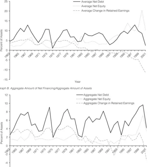
In Figure 1, the average ratios are the annual averages of net financing scaled by beginning-of-year assets (in percent), and the aggregate ratios are the annual aggregate amount of net financing of all firms scaled by the aggregate amount of beginning-of-year total assets (in percent). Figure 1 shows that the average net debt increase exceeded 10% of beginning-of-year assets in eight years. The average net equity issuance exceeded 6% in 12 years. The average change in retained earnings shows a declining trend, with the lowest value in 2001, the last year of our sample period. The aggregate net debt and equity issuances fluctuate substantially, with aggregate net external equity issuance peaking at over 7% of aggregate assets in 2000. The static trade-off theory has been unable to provide a satisfactory explanation for the magnitude of these fluctuations. The pecking
2Format code 5 is for Canadian firms, and format codes 4 and 6 are not defined in Compustat. 3To further reduce the effect of outliers, we also drop firm-year observations with book leverage
or market leverage that is negative or greater than one and Tobin’s Q that is negative or greater than 10. These variables will be defined later. Our results are robust to whether or not we keep these firm-year observations.
4We exclude 201 such firm years identified with Compustat footnote codes. The Financial
Ac-counting Standards Board (FASB) issued SFAS No. 94 in late 1987. Heavy equipment manufacturers and merchandise retailers were most affected by the standard because they made extensive use of unconsolidated finance subsidiaries. For example, Ford, General Motors, General Electric, and Inter-national Business Machines all had a huge increase in debt on their balance sheets from fiscal year 1987 to 1988. More specifically, Ford had a debt increase of about $93.8 billion, while its end-of-year total assets were $45.0 billion in 1987 and $143.4 billion in 1988, largely because Ford Credit was consolidated under the new standard. This standard also caused some firms to divest themselves of unconsolidated subsidiaries because otherwise they would violate debt covenant agreements on the maximum amount of leverage, and their returns on assets would appear too low and financial leverage would appear too high.
5When the liquidating value of preferred stock (item 10) is missing, we use the redemption value
of preferred stock (56). When the redemption value is also missing, we use the carrying value of pre-ferred stock (130). As one referee noted, convertible prepre-ferred stock is more equity-like than straight preferred stock. In unreported analysis we include the change in the carrying value of convertible preferred stock (214) in our definition of net equity. Our results remain qualitatively the same.
FIGURE 1
Average and Aggregate Financing Activities from the Balance Sheet
Net debt is the change in debt and preferred stock (Compustat items 181 + 10−35−79). Net equity is the change in equity and convertible debt (items 6−181−10 + 35 + 79) minus the change in retained earnings (36). Graph A of Figure 1 shows the equally weighted annual averages of net financing scaled by beginning-of-year assets of each firm (in percent). Graph B shows the annual aggregate amount of net financing of all firms in the sample scaled by the aggregate amount of beginning-of-year assets (in percent).
Graph A. Equally Weighted Averages of Net Financing/Assets
Graph B. Aggregate Amount of Net Financing/Aggregate Amount of Assets
order theory gains some support during 1974–1978, when the average net equity issuance was below 2%. As so often happens, however, the pattern on which the pecking order hypothesis was based began to break down shortly after the publication of Myers (1984).
Figure 1 understates securities issues because other firms that are retiring debt or buying back stock lower the averages. Table 1 reports the percentage of firms that are net securities issuers. Issuing firms in a year are defined as those for
TABLE 1
Percent of Firms in Different Financing Groups across Time
A firm is defined as issuing debt ifΔDscaled by beginning-of-year assets is at least 5%, whereΔDis the change in debt and preferred stock (Compustat items 181 + 10−35−79) from yeart−1 to yeart, or issuing equity ifΔEscaled by beginning-of-year assets is at least 5%, whereΔEis the change in equity and convertible debt (6−181−10 + 35 + 79) minus the change in retained earnings (36). The percentages of debt and equity issuers do not necessarily add up to 100 because firms can issue both debt and equity or neither debt nor equity. Firms with beginning-of-year assets of less than $10 million (1998 purchasing power) are excluded.
Year Total Number of Firms Debt Issues (%) Equity Issues (%)
1963 129 33.3 16.3 1964 465 35.7 12.0 1965 558 45.9 14.3 1966 722 54.2 16.3 1967 1,316 43.8 16.6 1968 1,570 53.9 24.5 1969 1,929 47.4 34.1 1970 2,211 40.9 14.7 1971 2,493 33.8 14.4 1972 2,739 43.0 16.7 1973 2,986 58.6 10.4 1974 3,039 57.9 6.8 1975 3,097 28.1 6.6 1976 3,046 38.6 8.1 1977 2,986 46.9 7.9 1978 2,875 57.7 9.5 1979 2,905 56.9 11.6 1980 2,975 45.5 15.4 1981 2,915 42.4 19.3 1982 3,073 34.8 13.1 1983 3,065 35.7 23.1 1984 3,146 45.3 17.7 1985 3,210 40.2 16.4 1986 3,079 39.6 19.4 1987 3,104 43.9 19.8 1988 3,097 44.4 14.8 1989 3,075 41.2 14.7 1990 3,063 39.7 13.5 1991 3,041 30.6 16.2 1992 3,133 35.8 21.8 1993 3,380 40.2 24.0 1994 3,715 45.0 24.5 1995 3,944 47.6 25.2 1996 4,214 43.5 29.7 1997 4,543 44.8 29.5 1998 4,564 49.5 27.4 1999 4,366 44.7 26.7 2000 4,202 43.1 31.5 2001 4,160 28.4 27.7
which debt or equity increases by more than 5% of beginning-of-year assets, the same definition that has been used, for example, in Hovakimian, Hovakimian, and Tehranian (2004) and Korajczyk and Levy (2003). Once we separate firms with net securities issues from other firms, we see a higher frequency of issuing. The percentage of firms with net debt issuance of at least 5% of assets is never below 28%. The pecking order theory predicts that equity issues will be rare. However, the proportion of net equity issuers (firms issuing at least 5% of assets) never drops below 6.6% in any year, peaks at over 34% in 1969, and is at least 25% in each year from 1995 to 2001.6
6Our proportion of equity issuers is much higher than in studies such as Jung, Kim, and Stulz
(1996) and DeAngelo, DeAngelo, and Stulz (2009), which define an equity issuer as a firm conducting a public seasoned equity offering for cash. Our definition of an equity issuer, which is standard in the empirical capital structure literature, includes firms that conduct private placements of equity or stock-financed acquisitions that increase the book value of equity by at least 5% of assets, net of share repurchases.
Overall, our summary statistics of financing activities cast doubt on the abil-ity of the pecking order model to describe most of the observed capital structures, consistent with Fama and French (2002), (2005), Frank and Goyal (2003), and Hovakimian (2006).
C. Summary Statistics of Macroeconomic Variables
How do firms judge the relative cost of equity? On the one hand, some firm executives may possess private information that is not reflected in market prices about their firms or their industries. On the other hand, they may follow certain psychological patterns. For example, reference points, as suggested by prospect theory, may play a role.7Alternatively, they may issue equity to take advantage
of publicly observable misvaluations if the equity market becomes temporarily overvalued (Stein (1996)).
Our proxy for the cost of equity is the implied ERP, estimated using analyst earnings forecasts (earnings per share (EPS) and LTG rate) at the end of the pre-vious calendar year for the 30 stocks in the Dow Jones Industrial Average.8The implied ERP is defined as the real internal rate of return that equates the current stock price to the present value of all future cash flows to common sharehold-ers of the firm (measured as book value of equity plus forecasted future residual earnings), minus the real risk-free rate (see Appendix A for details). Although they differ in their specific procedures, this is the general approach used by Claus and Thomas (2001), Gebhardt, Lee, and Swaminathan (2001), and Ritter and Warr (2002).9We follow Ritter and Warr (2002) to correct for inflation-induced
distortions in the estimation of the implied ERP. The equally weighted average of
7Casual conversations with investment bankers suggest that when they advise their clients on
the choice between debt and external equity financing, the most important factors they consider are whether a client’s stock price is near a 52-week high and whether the earnings yield on the stock is below the interest rate on debt.
8By using the lagged year-end values during yeartfor a firm with a Dec. 31 fiscal year, we are
using the Dec. 31 of yeart−1 accounting information and stock price. For a firm with a June 30 fiscal year, during yeartwe use the June 30 of yeart−1 accounting information and Dec. 31 of year t−1 stock price. We use forecasts from Value Line for 1968–1976 and from Institutional Brokers’ Estimate System (IBES) for 1977–2001. We hand-collect Value Line data fromValue Line Investment Surveyfor early years when the IBES database is not available. Because previous studies document that IBES and Value Line analysts make systematically different forecasts, we estimate the implied ERP for 1977 using analyst forecasts from both sources and then adjust the implied ERP for 1968– 1976 by multiplying the Value Line forecast by the ratio of the 1977 premium using IBES to the 1977 premium using Value Line. Brav, Lehavy, and Michaely (2005) estimate the implied nominal expected market return using target prices and future dividends from Value Line for 1975–2001. They estimate annual nominal expected returns varying from 34.1% in 1975 to 12.1% in 1997. Using their series instead of ours does not change our major results. Our qualitative results are also robust to using the value-weighted book-to-market ratio of equity for all NYSE-listed firms as a proxy for the relative cost of equity rather than the implied ERP.
9Consistent with the literature, we assume that analyst EPS forecasts are exogenous. Bayesian
an-alysts, however, may become overly conservative in their forecasts of EPS when the cost of equity is high, and overly optimistic when the cost of equity is low. This is because the market price implies fu-ture earnings, and a Bayesian analyst will incorporate these into his or her own forecasts. Furthermore, when P/E ratios are high, more optimistic forecasts are necessary in order to justify “buy” recommen-dations. The endogeneity results in a dampening of the time series of the implied ERP relative to its true fluctuations and hence creates a bias against our results.
the implied ERP for each of the Dow 30 stocks is used as an estimate of the ERP for the market. The time-variation of the implied ERP may be due to either the time-variation of risk, or of the risk aversion of investors (rational reasons), or to the time-variation of investor sentiment (an irrational reason).
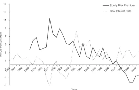
Figure 2 shows the real interest rate (RIR) and the implied ERP at the end of each calendar year. The ERP turned negative during 1996–2001, suggesting over-valuation of the stock market.10 Firms display a high propensity to issue equity during these years, as indicated in Table 1.
FIGURE 2
Equity Risk Premium and Real Interest Rate
The market equity risk premium is estimated using analyst forecasts at the year-end for the Dow 30 stocks from Value Line for 1968–1976 and from IBES for 1977–2001. The real interest rate is the nominal interest rate minus inflation, where the nominal interest rate is the yield on one-year Treasury bills in the secondary market at the beginning of each calendar year at http://www.federalreserve.gov/, and inflation is the rate of change of the consumer price index during the calendar year from CRSP.
Figure 2 also shows that the RIR was very low in 1973–1974 and 1978–1979, when the percentage of sample firms issuing debt rose to historic highs (over 56%
10Although we estimate a negative ERP for some years, our qualitative results are not dependent
on the ERPs being negative. The residual income methodology that we employ states that the value of equity is equal to the book value of equity plus the present value of future residual income (economic profits). Because we assume that future residual income is mean-reverting, a large present value of future residual income can only be achieved by using a low discount rate (i.e., since the numerator converges to zero, a small denominator is needed to generate a high ratio). When both the market-to-book ratio and the RIR are high, as was the case in the 1996–2001 period, the model produces a negative implied ERP. Some have argued that a high market-to-book ratio has existed in most years after 1995 because the book value of equity increasingly underrepresents the value of assets in place as intangibles represent more and more of firm value. If so, our estimates may overstate the downtrend in the ERP, and the true ERP may not be as negative as we estimate. Since we use the ERP as an explanatory variable, overestimating its decline would lead to underestimating the slope coefficient on the ERP.
for each of these years in Table 1). The RIR is used as a proxy for the time-varying cost of debt perceived by corporate executives.
Previous studies also use the term spread and the default spread as proxies for the costs of various forms of debt (e.g., Baker, Greenwood, and Wurgler (2003)). It is likely that the varying default risk premium can help explain the time-varying financing decisions. We thus include the default spread, which is defined as the difference in yields between Moody’s Baa- and Aaa-rated corporate bonds. The term spread, defined as the difference in yields between 10- and one-year Treasuries, is also included because firms might increase the use of long-term debt when the term spread is low.
We also include contemporaneous measures of the statutory corporate tax rate and the real gross domestic product (GDP) growth rate. The statutory cor-porate tax rate has changed over time and may have a major influence on the financing decisions of U.S. firms (see, among others, Graham (2003) and Kale, Noe, and Ramirez (1991)).11 The real GDP growth rate controls for growth
op-portunities. To the degree that these variables are important and have the expected signs, this lends support to the static trade-off model.
The lagged average announcement effect on seasoned equity offerings (SEOs) is included to see whether, as implied by the pecking order theory, time-varying information asymmetry is able to explain time-varying financing activities. Since the pecking order theory assumes that markets are semi-strong-form efficient, the announcement effect associated with equity issues is the primary proxy for the level of information asymmetry (Bayless and Chaplinsky (1996)).
Table 2 reports summary statistics for our proxies for market conditions. The implied ERP is positively correlated with the default spread and the statutory corporate tax rate and is negatively correlated with the RIR.
III.
Market Timing and Securities Issuance Decisions
How important are market conditions, especially the ERP, in securities is-suance decisions? This section reports and discusses the results from i) annual OLS regressions using a firm’s net debt issuance as the dependent variable and its net financing deficit as the independent variable, ii) pooled OLS regressions linking the pecking order slope coefficient to the time-varying cost of capital, and iii) a pooled nested logit regression for the joint decision of whether to issue securities and which security to issue.
A. Pecking Order Tests
Following Shyam-Sunder and Myers (1999), we first estimate
ΔDit = at+btDEFit+uit, (1)
11The statutory corporate tax rate was 52% in 1963, 50% in 1964, 48% in 1965–1967, 52.8% in
1968–1969, 49.2% in 1970, 48% in 1971–1978, 46% in 1979–1986, 40% in 1987, 34% in 1988–1992, and 35% in 1993–2001.
TABLE 2
Summary Statistics of Macroeconomic Variables
ERPt−1is the implied market equity risk premium at the end of yeart−1, estimated using analyst forecasts for the Dow 30 stocks from Value Line for 1968–1976 and from IBES for 1977–2001. RIRt−1is the nominal interest rate minus realized inflation, where the nominal interest rate is the yield (daily series) on one-year Treasury bills in the secondary market at the end of yeart−1 at http://www.federalreserve.gov/, and inflation is the rate of change of the consumer price index during yeartfrom CRSP. DSPt−1is the default spread, defined as the difference in yields (weekly series, since daily series only goes back to 1983) between Moody’s Baa-rated and Aaa-rated corporate bonds at the end of yeart−1. TSPt−1is the term spread, defined as the difference in yields (daily series) between 10- and one-year constant maturity Treasuries at the end of yeart−1. TAXRtis the statutory corporate tax rate during yeart. RGDPtis the real GDP growth rate during year tfrom the Bureau of Economic Analysis, Department of Commerce. RSEOt−1is the annual average of market-adjusted returns during yeart−1 from one day before to one day after the file date of seasoned equity offerings (SEOs), computed by the authors using SEO data from Thomson Financial. The average announcement effect is calculated from 1980, the first year the file date is available for most SEOs. Subscripttdenotes the current year andt−1 denotes the previous year. TAXR, RGDP, and RIR are available for 1963–2001. ***, **, and * denote statistical significance at the 1%, 5%, and 10% levels, respectively, in a two-tailed test.
ERPt−1 RIRt−1 DSPt−1 TSPt−1 TAXRt RGDPt RSEOt−1
N 33 39 39 39 39 39 21 Mean 0.031 0.016 0.011 0.007 0.430 0.033 −0.018 Std Dev 0.037 0.027 0.005 0.011 0.067 0.022 0.005 Min −0.043 −0.054 0.003 −0.014 0.340 −0.020 −0.028 Median 0.037 0.016 0.009 0.006 0.460 0.036 −0.017 Max 0.114 0.083 0.024 0.031 0.528 0.073 −0.008 Correlation ERPt−1 1 RIRt−1 −0.316* 1 DSPt−1 0.469*** 0.346** 1 TSPt−1 −0.058 0.218 0.117 1 TAXRt 0.705*** −0.257 0.126 −0.255 1 RGDPt −0.181 −0.035 −0.376** 0.291* 0.158 1 RSEOt−1 0.191 0.259 0.422* −0.273 0.420* 0.077 1
whereΔDitis the change in book debt as a percentage of beginning-of-year as-sets for firmiat the end of the fiscal year ending in calendar yeart, and DEFit is the change in assets minus the change in retained earnings as a percentage of beginning-of-year assets. To examine how the slope coefficient on the financing deficit has changed across time, we estimate this equation each year. The esti-mated slope coefficient, ˆb, known as the pecking order coefficient, shows very interesting time-series patterns and is reported in Figure 3. It ranges from 0.67 to 0.92 in the 1960s and the 1970s, from 0.48 to 0.79 in the 1980s, and from 0.27 to 0.58 from 1990 to 2001. Frank and Goyal (2003) find that the slope coefficient was low in the 1990s as well. However, a time trend does not explain everything. Even within each decade, there are ups and downs that might be explained with our proxy for the relative cost of equity capital.
Since the effect of market conditions on a negative financing deficit is un-clear, we focus on the effect of market conditions on a positive financing deficit by estimating the following regression, pooling all firm year observations:
ΔDit = a+bNDEFit+(c+dERPt−1+eRIRt−1+fDSPt−1+gTSPt−1
(2)
+hTAXRt+jRGDPt+kRSEOt−1)×PDEFit+εit,
where NDEFit equals DEFit if DEFit < 0 and zero otherwise; PDEFit equals DEFitif DEFit>0 and zero otherwise; ERPt−1is the implied market ERP at the
end of yeart−1; RIRt−1is the expected real interest rate at the end of yeart−1;
DSPt−1 is the default spread at the end of yeart−1; TSPt−1 is the term spread
FIGURE 3
Pecking Order Slope Coefficients
Coefficients are computed annually by estimating equation (1).
RGDPt is the real GDP growth rate during year t; and RSEOt−1 is the annual
average of market-adjusted returns for the three-day window[−1,+1]surrounding the file date of SEOs during yeart−1 (SEO data is from Thomson Financial’s new issues database). The market timing theory predicts a positive coefficient on the interaction between the ERP and the positive financing deficit. Results are reported in Table 3. Correlation of the observations across time for a given firm and correlation across firms for a given year could result in biased standard errors in our panel data set regressions. Consequently, we reportt-statistics using standard errors corrected for clustering by both firm and year (Petersen (2009)).12
Consistent with the market timing theory, firms finance a large proportion of their financing deficit with net external equity when the cost of equity is low. In Panel A of Table 3, we follow Baker and Wurgler (2002) to define the financing deficit as including dividends and the change in cash (i.e., higher dividends in-crease the financing deficit). In regression (1), the implied ERP at the end of year t−1 is positively related to the pecking order coefficient in yeart. In economic terms, a one-standard-deviation (0.037) increase in the implied ERP is associated with 10.8% more of the financing deficit being funded with net debt (for exam-ple, increasing from 60% to 70.8%). Elliott, Koeter-Kant, and Warr (2007) also
12Petersen (2009) suggests that the Rogers (1993) standard errors clustered by firm and by year
are more accurate than uncorrected standard errors in the presence of both firm and year correlations in a panel data set. The existing STATA software does not have a built-in command to correct for two-dimensional clustering (for example, clustering by both firm and year). However, Mitchell Pe-tersen kindly provides a STATA ado file used in PePe-tersen (2009) for two-dimensional clustering (see http://www.kellogg.northwestern.edu/faculty/petersen/htm/papers/se/se programming.htm).
TABLE 3
Market Conditions and the Funding of the Financing Deficit
The following equation is estimated:
ΔDit = a+bNDEFit+(c+dERPt−1+eRIRt−1+fDSPt−1+gTSPt−1+hTAXRt
+jRGDPt+kRSEOt−1)×PDEFit+εit.
In Panel A of Table 3, the financing deficit, DEFit, is defined asΔDit+ΔEit, whereΔDitis the change in debt and preferred stock (Compustat items 181 + 10−35−79) from yeart−1 to yeartas a percentage of beginning-of-year assets for firmi, andΔEitis the change in equity and convertible debt (items 6−181−10 + 35 + 79) minus the change in retained earnings (item 36) as a percentage of beginning-of-year assets. In Panel B, the financing deficit excludes dividends (item 127) and the change in cash (item 1). In both panels, NDEFitequals DEFitif the deficit is negative and zero otherwise, and PDEFit equals DEFitif the deficit is positive and zero otherwise. The standard deviations of PDEFitare 35.9% for the sample used in regressions (1) and (2) of Panel A, 40.8% for the sample used in regression (3) of Panel A, 31.9% for regressions (1) and (2) of Panel B, and 35.9% for regression (3) of Panel B. ERPt−1is the implied market equity risk premium at the end of yeart−1. RIRt−1is the nominal interest rate minus inflation in yeart. DSPt−1is the default spread, defined as the difference in yields between Moody’s Baa-rated and Aaa-rated corporate bonds at the end of yeart−1. TSPt−1is the term spread, defined as the difference in yields (daily series) between 10- and one-year constant maturity Treasuries at the end of yeart−1. TAXRtis the statutory corporate tax rate during yeart. RGDPtis the real GDP growth rate during yeart. RSEOt−1is the annual average of market-adjusted returns during yeart−1 from one day before to one day after the file date of seasoned equity offerings (SEOs). The average announcement effect is calculated from 1980, the first year the file date is available for most SEOs. All of the macroeconomic variables are presented in decimal form (i.e., a 5% ERP is presented as 0.05). Both the dependent variable and the financing deficit are presented as percentages. In each regression, we exclude firm year observations where|ΔDit|>400% or|ΔEit|>400%. Thet-statistics are corrected for correlation both across observations of a given firm and across observations of a given year (Rogers (1993)) and for heteroskedasticity (White (1980)).
(1) (2) (3)
1969–2001 1969–2001 1981–2001
Coeff. t-Stat. Coeff. t-Stat. Coeff. t-Stat.
NDEFit 0.71 17.18 0.70 17.41 0.68 15.33 PDEFit 0.50 24.22 0.27 1.65 0.33 1.79 ERPt−1×PDEFit 2.91 5.06 3.06 3.99 2.95 4.32 RIRt−1×PDEFit −0.56 −0.86 1.33 1.11 DSPt−1×PDEFit −2.03 −0.42 6.30 0.83 TSPt−1×PDEFit −3.70 −2.52 −3.67 −2.34 TAXRt×PDEFit 0.50 1.13 −0.53 −0.86 RGDPt×PDEFit 3.09 2.67 5.12 3.81 RSEOt−1×PDEFit −6.06 −3.33 Constant 0.70 2.96 0.51 2.46 0.85 3.96 Adj.R2 0.648 0.657 0.625 N 112,483 112,483 78,696 NDEFit 0.40 10.38 0.39 10.30 0.37 8.81 PDEFit 0.59 37.78 0.45 4.79 0.46 5.00 ERPt−1×PDEFit 3.14 7.42 3.27 6.44 3.36 7.14 RIRt−1×PDEFit −0.45 −1.03 0.74 1.04 DSPt−1×PDEFit 1.52 0.57 5.80 2.06 TSPt−1×PDEFit −3.42 −3.15 −3.54 −2.93 TAXRt×PDEFit 0.19 0.64 −0.35 −1.03 RGDPt×PDEFit 2.90 3.07 4.28 4.55 RSEOt−1×PDEFit −3.32 −2.90 Constant −0.14 −0.69 −0.21 −1.17 −0.44 −2.52 R2 0.676 0.681 0.664 N 112,467 112,467 78,682
Panel A. Financing Deficit (defined with dividend payments increasing the deficit)
Panel B. Financing Deficit (defined with dividend payments not affecting the value of the deficit)
relate the pecking order slope coefficient to the ERP estimated for each firm and find qualitatively similar results. Our estimate of the ERP at the market level using only the well-established Dow 30 companies with reliable accounting information is relatively conservative and is likely to understate the importance of valuation in the choice between debt and equity.
In regression (2) the estimated coefficient on the interaction between the ERP and the positive financing deficit changes little after controlling for the real rate of return on debt, the default spread, the term spread, the statutory tax rate, and the real GDP growth rate. The regression also shows that firms fund a larger
proportion of their financing deficit with net debt when the corporate tax rate is higher, consistent with the trade-off theory prediction that debt is used as a tax shield, although the relation is not statistically significant. The coefficient on the interaction between the real rate of GDP growth and the positive financing deficit is positive and statistically significant, suggesting that firms are more likely to fund their current growth opportunities with debt.
Regression (3) in Table 3 includes the average announcement effect of SEOs as an explanatory variable, using a shorter sample period because our RSEO se-ries does not begin until 1980. This variable measures the adverse selection costs of issuing equity, and has been used by, among others, Korajczyk, Lucas, and McDonald (1990), Choe, Masulis, and Nanda (1993), Bayless and Chaplinsky (1996), and Korajczyk and Levy (2003). The significantly negative sign of the interaction between the average announcement effect and the positive financing deficit is consistent with previous studies. That is, when this negative number is closer to zero, firms issue more equity. Economically, a one-standard-deviation (0.005) increase in the average announcement effect results in a decrease of 3.0% of the financing deficit being funded with net debt. Relative to the impact of the ERP, the average announcement effect (and therefore time-varying asymmetric in-formation) is of secondary importance in the choice of debt and equity financing. If a firm pays out the cash flow it generated as a dividend, then the financing deficit as defined in Panel A of Table 3 does not include that cash flow because both assets and retained earnings are decreased by the dividend. However, if the firm engages in a stock repurchase, then the financing deficit includes the cash flow because the deficit measures net external financing. In Panel B, we exclude dividends and the change in cash in the definition of the financing deficit (i.e., the payment of dividends does not affect the value of the financing deficit). The coefficient on the interaction between the ERP and the positive financing deficit becomes even larger, suggesting a greater role of the ERP in the choice between external debt and external equity to fund the financing deficit.
The regression approach has both advantages and disadvantages. The ad-vantages include the summarization of information in the pecking order slope coefficient, convenience for analyzing a large number of firms, and convenience for controlling for other factors in a multivariate framework. The disadvantages include the potentially large influence of a few outliers and the oversimplification of information. Furthermore, Chirinko and Singha (2000) question the validity of Shyam-Sunder and Myers’ (1999) pecking order tests.
To gain additional insight, in Figure 4 we randomly select 100 firms each year and draw scatter-plots. We limit the number of randomly selected firms to 100 per year because a larger number makes it difficult to visually identify mean-ingful patterns. If a firm funds 100% of its financing deficit with net debt, all of the points plotted will lie on the 45◦line. A firm with negative net equity issuance will lie on the left-hand side of the 45◦line, while a firm with positive net equity issuance will lie on the right-hand side of the 45◦line. We report the scatter-plots for only four years because those for other years with similar slope coefficients are qualitatively the same. In 1975, when the slope coefficient is 0.91, only a small number of firms deviate from the 45◦line. In 1992, however, when the slope co-efficient is 0.42, several percent of the points are far to the right of the 45◦line.
FIGURE 4
Scatter-Plots of Net Debt versus Net External Financing
The horizontal axis denotes net external financing scaled by beginning-of-year assets, and the vertical axis denotes net debt scaled by beginning-of-year assets. For each selected year, 100 randomly selected observations are plotted. The pecking order slope coefficient in Figure 3 is 0.909 for 1975, 0.768 for 1982, 0.482 for 1983, and 0.423 for 1992.
These firms issue a lot of equity to finance their financing deficit or to retire debt. Only a few firms are noticeably to the left of the 45◦ line, suggesting that firms only infrequently repurchase shares in a quantitatively important manner.
B. Nested Logit Model for the Joint Decision
In the pecking order tests, we assume that the financing deficit is exogenous. However, a firm may decide jointly whether to issue securities and which secu-rity to issue. Therefore, we also estimate a nested logit model (Greene (2003), pp. 725–727), as do Gomes and Phillips (2007).13 The nested logit model can
also potentially reduce the large influence of a few firms raising a large amount of debt or equity on the pecking order slope coefficient, because firms issuing 6% or
13A nested logit model is similar to a multinomial logit model. However, a multinomial logit model
assumes that choices between any two alternatives are independent of the other alternatives, while a nested logit model only assumes that the choices are independent within a group or “nest” of alterna-tives.
60% of assets are both assigned the same value in the nested logit model. Another concern regarding the pecking order tests is that the estimated coefficient from the financing deficit may simply reflect changing firm characteristics rather than changing market conditions (Flannery and Rangan (2006)). We control for firm characteristics in the nested logit model.
Our nested logit model includes two decision levels. The first-level alter-natives are security issuance versus no security issuance, and the second-level alternatives are equity versus debt issuance. Let Pr(i)equal either the probability of security issuance (i=s) or the probability of no security issuance (i=n), and Pr(j|s) equal either the probability of equity issuance (j=e) or the probability of debt issuance (j=d) conditional oni=s.14Then
Pr(j|s) = exp(xsjβ) exp(xseβ)+ exp(xsdβ) (3)
and
Pr(s) = exp(ysα+ηsIs)
exp(ysα+ηsIs)+ exp(ynα+ηnIn), (4)
where the inclusive valuesIi=ln{exp(xieβ)+ exp(xidβ)},xij, andyirefer to the row vectors of explanatory variables specific to categories (i,j) and (i), respec-tively, and ηi refers to the inclusive parameters. We use nonissuers as the base alternative at the first decision level, and debt issuers as the base alternative at the second decision level. The nested logit model is estimated using full-information maximum likelihood.15
We use the same set of explanatory variables, including both firm charac-teristics and market conditions, for all alternatives.16Firm characteristics include
financial slack (the sum of cash and short-term investments), profitability, capital expenditures, Tobin’s Q (market-to-book ratio of assets), R&D expenditures, the logarithm of net sales, the logarithm of the number of years the firm has been listed on CRSP, the lagged leverage, the market-adjusted return during the previ-ous fiscal year, and the market-adjusted return during the following three fiscal years. The results for the nested logit model are reported in Table 4.17 To
as-sist in gauging economic significance, we vary each explanatory variable by plus or minus one standard deviation from its sample value (a two-standard-deviation change), and then we average the change in the predicted probability over all firms in the sample in order to obtain the economic effects, holding other variables
14A firm is defined as issuing debt if the net change in debt is at least 5% of its
beginning-of-year assets. Similarly, a firm is defined as issuing equity if the net change in equity is at least 5% of its beginning-of-year assets. For convenience, firm years when both debt and equity are issued are excluded in the nested logit regressions. For characteristics of firms issuing both debt and equity, see Hovakimian et al. (2004). We keep these firms in other analyses.
15Several previous studies examine the choice between debt versus equity financing in isolation
using a logit model (e.g., Jung et al. (1996)) or a probit model (e.g., Mackie-Mason (1990)), implicitly assuming that the choice between issuing versus not issuing security is exogenous.
16If we restrict bothη
s=1 andηn=1, then we have a multinomial logit model.
17We are not aware of any statistical packages that are able to adjust nested logit regressions for
TABLE 4
Nested Logit Model of Securities Issuance Decisions
We estimate a nested logit model of the following structure:
We use nonissuers as the base alternative at the first decision level, and debt issuers as the base alternative at the second decision level. Firms that issue both debt and equity in the same year are excluded from the sample, which covers 1969– 2001.ΔDis the change in debt and preferred stock (Compustat items 181 + 10−35−79).ΔEis the change in equity and convertible debt (items 6−181−10 + 35 + 79) minus the change in retained earnings (36). A firm is defined as issuing debt ifΔD/At−1≥0.05. Similarly, a firm is defined as issuing equity ifΔE/At−1≥0.05. CASH is the sum of cash and short-term investments (1) scaled by assets. OIBD is operating income before depreciation (13) scaled by assets. CAPEX is the capital expenditure (128) scaled by assets. Q is the sum of the market value of equity and the book value of debt divided by the book value of assets. R&D is the research and development expense (46) scaled by assets and is set to zero if it is missing. R&DD is a dummy variable that equals one if R&D is missing and equals zero otherwise. SALE is the log of net sales (12). AGE is the natural log of the number of years the firm has been listed on CRSP. BL is book leverage, defined as book debt (items 181 + 10−35−79) scaled by assets. MARt−1is measured as the difference between the firm raw return and the value-weighted market return in the preceding fiscal year. MARt+1,t+3is measured as the difference between the firm raw return and the value-weighted market return in the following three fiscal years. If a firm is delisted, its post-event three-year raw return is calculated by compounding the CRSP value-weighted market return for the remaining months. ERPt−1is the implied market equity risk premium at the end of yeart−1. RIRt−1is the nominal interest rate minus inflation in yeart. DSPt−1is the default spread, defined as the difference in yields between Moody’s Baa-rated and Aaa-rated corporate bonds at the end of yeart−1. TSPt−1is the term spread, defined as the difference in yields (daily series) between 10- and one-year constant maturity Treasuries at the end of yeart−1. TAXRtis the statutory corporate tax rate during yeart. RGDPtis the real GDP growth rate during yeart. To help gauge the economic effects, we vary each explanatory variable from one standard deviation below to one standard deviation above its sample value, and use the coefficients from the nested logit regression to calculate the change in the predicted probability, holding all other variables fixed. We then average the change in the predicted probability over all firms in the sample to get economic effects. Thet-statistics are calculated using heteroskedastic consistent standard errors (White (1980)).
First-Level Decision: Second-Level Decision:
Issuing (vs. Not Issuing) Equity (vs. Debt)
Economic Economic
Coeff. t-Stat. Effect Coeff. t-Stat. Effect
CASHit−1 −1.051 −15.59 −7.1% 0.369 3.88 2.1% OIBDit−1 −0.793 −7.15 −4.5% −1.218 −10.50 −5.6% CAPEXit−1 3.213 27.17 11.3% 0.919 7.01 2.7% Qit−1 0.341 16.17 15.9% 0.384 28.62 14.7% R&DDit−1 0.071 3.86 1.6% 0.236 9.35 4.3% R&Dit−1 1.565 6.24 4.7% 3.452 14.07 8.3% SALEit−1 0.002 0.36 0.1% −0.134 −17.20 −9.3% AGEit −0.228 −20.32 −8.4% −0.107 −6.33 −3.2% BLit−1 0.177 3.17 1.6% 1.035 15.39 7.6% MARit−1 0.477 22.12 14.8% 0.384 21.08 9.9% MARit+1,t+3 −0.068 −11.67 −5.1% −0.106 −11.93 −6.5% ERPt−1 −3.164 −7.92 −5.4% −7.462 −13.30 −10.3% RIRt−1 −3.488 −9.36 −4.6% 3.510 6.36 3.8% DSPt−1 −13.417 −5.55 −3.0% 17.005 4.86 3.2% TSPt−1 −8.514 −11.14 −4.4% 3.889 3.31 1.7% TAXRt 1.271 6.44 3.7% 0.835 2.83 2.0% RGDPt 4.452 9.71 4.2% −4.324 −6.04 −3.4% N 82,653
fixed. Because our results are generally consistent with other results in the litera-ture, we will only highlight a few of the results.
We first briefly discuss results for the first-level decision: security issuance versus no security issuance. Consistent with the pecking order theory, firms that have more cash and higher profitability are less likely to access external capi-tal markets, while growth firms, as measured by capicapi-tal expenditure, Tobin’s Q,
R&D, and the preissue one-year market-adjusted firm return, are more likely to access external markets. Older firms rely less on external financing. Macroeco-nomic variables also appear to be important determinants of whether to access external markets.
We proceed to discuss results for the second-level decision: equity issuance versus debt issuance, conditional on the decision of security issuance. Our results are generally consistent with the existing literature. Firms with more cash are more likely to issue equity. Profitable firms are more likely to issue debt. Firms with more growth opportunities, as measured by capital expenditure, Tobin’s Q, R&D, and preissue one-year market-adjusted return, are more likely to issue eq-uity. Larger and older firms are more likely to issue debt.
Confirming the importance of market timing, Tobin’s Q and the past market-adjusted firm return are among the most important explanatory variables in the decision to issue equity, both statistically and economically. Holding other vari-ables at their sample values, if Tobin’s Q is increased from one standard deviation below to one standard deviation above its sample value, the propensity to issue equity increases by 14.7%. Similarly, if the past market-adjusted firm return is increased from one standard deviation below to one standard deviation above its sample value, the propensity to issue equity increases by 9.9%. Firms that subse-quently underperform are also more likely to issue equity, and this variable has a larger economic significance than most other variables. An increase in the future market-adjusted return from one standard deviation below to one standard devi-ation above results in almost a 6.5% reduction in the propensity to issue equity. This provides further support for the market timing theory.18
Consistent with the static trade-off theory, high leverage firms are more likely to issue equity rather than debt during 1964–2001. If we increase the lagged book leverage from one standard deviation below to one standard deviation above its sample value, the propensity to issue equity increases by 7.6%.
We are interested in whether the implied ERP has additional explanatory power after controlling for firm characteristics. If the lagged value of the ERP increases from one standard deviation below to one standard deviation above its sample value, the average propensity to issue equity instead of debt decreases by 10.3%. Economically, it is more significant than all other variables except the lagged firm level Tobin’s Q.
When the RIR is higher, firms are more likely to issue equity. Economically, an increase from one standard deviation below to one standard deviation above
18Jung et al. (1996) include the post-issue firm return as a proxy for expected misvaluation in a logit
model for firms’ choice between debt and equity issuance, although they do not find this variable to be statistically significant for a small sample of U.S. firms from 1977 to 1984. Consistent with our results, DeAngelo et al. (2009) also find a statistically significant negative relation between the probability of conducting an SEO and future three-year market-adjusted returns for U.S. firms from 1982 to 2001. However, they find that the propensity to issue equity increases by only 1.5% for a swing of a 75% loss to a 75% gain over three subsequent years, far below our 6.5%. The difference in results appears to be primarily due to two reasons: i) The definitions of equity issuers are different. They use SEOs, whereas we use the change in the book value of equity (net of increases in retained earnings), which includes private placements and stock-financed acquisitions. ii) Their 1.5% is the percent of equity issuers among all firms, while our 6.5% is the percent of equity issuers among debt issuers and equity issuers.
its sample value is associated with an increase of 3.8% in the propensity to issue equity. The default and term spreads have an even more modest effect on the debt versus equity choice. Inconsistent with the static trade-off theory that views the tax rate as a major factor in the decision to issue debt, the tax rate has only a secondary effect on the propensity to issue debt or equity.
The statistical and economic importance of our cost of capital proxies is consistent with the hypothesis that firms time their securities offerings to take advantage of intertemporal variation in the relative cost of different sources of capital. One could also interpret these results as being consistent with the static trade-off model, with firms moving to a new optimum as the relative costs of debt and equity change. Traditionally, researchers have assumed that the relative costs do not vary over time. Instead, researchers have assumed that firm characteristics might change over time, but the market-determined costs of debt and equity do not change.
In summary, the nested logit results in Table 4 suggest that Tobin’s Q, the preissue stock price run-up, and the implied ERP are the three most important de-terminants of firms’ choice between equity and debt.19This is consistent with the
market timing theory, although not necessarily inconsistent with the static trade-off theory with an optimal target that depends on the time-varying relative costs of debt and equity and growth opportunities. To further distinguish the alternative theories, in the next section we investigate how historical market conditions influ-ence a firm’s current leverage through their important role in the firm’s historical financing activities.
IV.
Effects of Market Timing on Capital Structure
Firms may adjust their capital structure with internal funds or external funds. The pecking order theory posits that external funds are more expensive than in-ternal funds and exin-ternal equity is more expensive than exin-ternal debt. Therefore, securities issues, especially equity issues, should be rare and only have a material impact on the capital structure of firms with insufficient internal funds. The mar-ket timing theory is similar to the pecking order theory in that observed capital structure is the outcome of historical external financing decisions, rather than a primary goal in itself.
In contrast, in the static trade-off theory, firms issue securities to adjust to-ward their target leverage. Once target leverage and partial adjustment are prop-erly controlled for, past securities issues and market conditions should have no important impact on current leverage (although with adjustment costs, Fischer, Heinkel, and Zechner (1989), Hennessy and Whited (2005), Ju, Parrino, Poteshman, and Weisbach (2005), Leary and Roberts (2005), Strebulaev (2007),
19We did several robustness checks: i) using a multinomial logit model even if our unreported test
shows that choices between any two alternatives are not independent of the other alternatives; ii) using the value-weighted market-to-book ratio of equity of all NYSE-listed firms prior to fiscal yeartas an alternative proxy for the cost of equity at the market level; iii) including convertible preferred stock in equity; and iv) excluding firm-year observations with major mergers and acquisitions and spin-offs. Our results are not qualitatively affected.
and others allow for a role). Therefore, it is important to examine the effects of past securities issues and market conditions on observed capital structures in or-der to compare the relative strength of each theory. This is especially important because there is widespread agreement that market timing considerations appear to be important in determining securities issues (see Alti (2006) and Hovakimian (2004), (2006), among others). The main debate is regarding the persistence of the effects of securities issues and market conditions on capital structure.
To control for target leverage when estimating the effects of past securities issues on current leverage, we estimate the following regression:
Lit = f(TARGET LEVERAGE PROXIESit−1, PDEFit−k, (5)
ERPt−k−1×PDEFit−k),
whereLitis the leverage ratio of firmiat the end of yeart,kis the lag length in years, PDEFit−kequals DEFit−k if DEFit−k >0 and zero otherwise (DEFit−kis the change in assets minus the change in retained earnings scaled by beginning-of-year assets for firmiin yeart−k), and ERPt−k−1is the implied ERP at the end of
yeart−k−1. Target leverage proxies include lagged firm characteristics, lagged or current macroeconomic variables, and year dummies. We examine whether the ERPk+1 years ago and firmi’s financing deficitkyears ago still have an impact on the firm’s current leverage. The static trade-off theory predicts that the coefficients on ERPt−k−1×PDEFit−kand PDEFit−kshould be insignificant whenkis large. The market timing theory predicts that the effect of ERPt−k−1×PDEFit−kon yeart leverage should be positive and statistically significant untilkbecomes very large. Table 5 reports pooled OLS results with book leverage (Panel A) or market leverage (Panel B) as the dependent variable fork=0, 4, 6, and 8. To remove the effects of clustering on the estimated standard errors, we reportt-statistics corrected for correlation both across observations of a given firm and across ob-servations of a given year (Petersen (2009)). Since the results regarding the target leverage proxies are generally consistent with previous studies, we focus our dis-cussions on the effects of the historical ERPs and financing deficits. Also, we focus our discussions on book leverage, since there is evidence that firms only slowly undo the effect on market leverage induced by stock price movements (Welch (2004)). In the market leverage regressions, the larget-statistics on Q are partly due to the mechanical relation induced by the market value of equity being in the numerator of Q and the denominator of the dependent variable.
The regression (1) results withk=0 are generally consistent with the results in Table 3. The coefficient on the interaction between the ERP and the financing deficit is statistically significant. The effect of the financing deficit on book lever-age is(3.687×ERPt−1+ 0.242)×PDEFit. Consistent with the market timing theory, the effect of the financing deficit on leverage is positively related to the implied ERP. The minimum estimated ERP is−0.043 (−4.3% per year) in 1999, and the maximum is 0.114 (11.4% per year) in 1974. For a firm with a financ-ing deficit of 10% (the sample mean) in 1999, the effect on its book leverage is
(3.687×(−0.043)+ 0.242)×10% = 0.83%. For a firm with a financing deficit of 10% in 1974, the effect on its book leverage is(3.687×0.114 + 0.242)×10% = 6.62%. Thus, the financing deficit results in a smaller increase in book leverage
TABLE 5
Effects of Historical Financing Activities and Market Conditions on Leverage
The following equation is estimated using firms from the period 1969–2001:
Lit = f(TARGET LEVERAGE PROXIESit−1,ERPt−k−1×PDEFit−k,PDEFit−k).
The dependent variable,Lit, is either book leverage or market leverage of firmiat the end of yeart. Book leverage is defined as book debt (items 181 + 10−35−79) divided by book assets (item 6). Market leverage is defined as book debt divided by market assets (items 181 + 10−35 + 25×199). Target proxies include firm characteristics, market conditions, and year dummies. Q is the sum of the market value of equity and the book value of debt divided by the book value of assets. R&D is the research and development expense (46) and is set to zero if it is missing. R&DD is a dummy variable that equals one if R&D is missing and equals zero otherwise. CAPEX is the capital expenditure (128). SALE is the log of net sales (12). OIBD is the operating income before depreciation (13). TANG is the net property, plant, and equipment (8). R&D, CAPEX, OIBD, and TANG are scaled by end-of-year assets. ERPt−k−1is the implied market equity risk premium at the end of yeart−k−1. RIRt−1is the nominal interest rate at the end of yeart−1 minus inflation in yeart. DSPt−1is the default spread at the end of yeart−1. TSPt−1is the term spread at the end of yeart−1. TAXRtis the statutory corporate tax rate during yeart. RGDPtis the real GDP growth rate during yeart. PDEFit−kis the positive financing deficit during fiscal yeart−k, scaled by total assets at the end of yeart. PDEFit−kequals zero if the financing deficit during fiscal yeart−kis negative. Firm year observations where PDEFit−k>10 are dropped. The standard deviations of PDEFit, PDEFit−4, PDEFit−6, and PDEFit−8are, respectively, 16.1%, 16.0%, 16.7%, and 18.2%. Year dummies and the intercept are included, but their coefficients are not reported. We reportt-statistics using standard errors corrected for correlation across both observations of a given firm and observations of a given year (Rogers (1993)).
(1) (2) (3) (4)
k=0 k=4 k=6 k=8
Coeff. t-Stat. Coeff. t-Stat. Coeff. t-Stat. Coeff. t-Stat. Panel A. Book Leverage
Qit−1 −0.037 −23.54 −0.030 −11.45 −0.026 −8.36 −0.023 −6.58 R&DDit−1 0.028 7.09 0.020 4.53 0.020 4.29 0.019 3.85 R&Dit−1 −0.456 −7.93 −0.480 −8.45 −0.486 −7.64 −0.498 −7.41 CAPEXit−1 0.055 1.86 0.126 2.38 0.108 2.14 0.083 1.57 SALEit−1 0.031 16.86 0.032 15.91 0.033 15.87 0.033 15.79 OIBDit−1 −0.347 −9.34 −0.439 −9.60 −0.488 −9.86 −0.524 −9.51 TANGit−1 0.002 0.13 −0.020 −1.44 −0.023 −1.68 −0.026 −1.76 ERPt−1 −0.479 −1.78 −0.284 −1.10 −0.476 −1.48 −0.332 −1.00 RIRt−1 0.189 1.17 0.256 1.43 0.317 1.88 0.390 2.26 DSPt−1 −0.198 −0.18 −0.514 −0.43 −0.528 −0.45 −0.325 −0.31 TSPt−1 0.037 0.10 −0.104 −0.27 −0.096 −0.26 −0.090 −0.20 TAXRt −0.525 −3.66 −0.474 −2.56 −0.506 −2.75 −0.606 −3.18 RGDPt −0.159 −0.80 −0.106 −0.48 −0.129 −0.50 −0.071 −0.27 ERPt−k−1×PDEFit−k 3.687 9.01 2.170 4.43 1.909 4.19 0.867 1.15 PDEFit−k 0.242 14.46 0.044 2.53 0.017 1.23 0.028 1.00
Year dummies Yes Yes Yes Yes
N 111,413 68,757 55,236 44,630
R2 0.217 0.182 0.181 0.179
Panel B. Market Leverage
Qit−1 −0.088 −26.50 −0.099 −19.12 −0.101 −19.19 −0.099 −18.75 R&DDit−1 0.026 5.74 0.018 3.60 0.017 3.20 0.016 2.99 R&Dit−1 −0.624 −10.38 −0.669 −11.93 −0.684 −11.31 −0.676 −10.72 CAPEXit−1 −0.066 −2.34 −0.044 −0.95 −0.043 −0.95 −0.041 −0.83 SALEit−1 0.021 21.51 0.021 17.33 0.021 16.22 0.022 14.78 OIBDit−1 −0.451 −8.82 −0.574 −9.27 −0.634 −10.08 −0.669 −10.54 TANGit−1 0.028 1.82 0.016 1.07 0.018 1.23 0.018 1.13 ERPt−1 −0.415 −1.41 −0.471 −1.93 −0.594 −1.70 −0.498 −1.31 RIRt−1 0.229 0.89 0.369 2.07 0.428 2.12 0.553 2.80 DSPt−1 −2.373 −1.75 −2.077 −1.55 −2.044 −1.35 −1.397 −1.10 TSPt−1 −0.265 −0.63 −0.129 −0.43 −0.169 −0.52 −0.188 −0.57 TAXRt −0.428 −2.01 −0.340 −1.50 −0.351 −1.49 −0.480 −2.11 RGDPt −0.523 −2.57 −0.523 −3.27 −0.569 −2.19 −0.436 −2.07 ERPt−k−1×PDEFit−k 1.388 3.78 1.905 3.96 2.146 4.49 0.754 1.04 PDEFit−k 0.136 9.77 0.015 0.79 −0.014 −0.91 0.016 0.61
Year dummies Yes Yes Yes Yes
N 111,413 68,757 55,236 44,630
when the cost of equity is low (1999) than when the cost of equity is high (1974), a pattern not predicted by the pecking order hypothesis. The total effect of the financing deficit on market leverage in Panel B also depends on the magnitude of the ERP, although the quantitative effect is smaller.
In regression (2) withk =4, the effect of the financing deficit five years ago on current book leverage is(2.170×ERPt−5+ 0.044)×PDEFit−4. For example,
a 10% financing deficit in 1996, when the implied ERP was low, would increase a firm’s book leverage five years later by only(2.170×(−0.004)+ 0.044)×10% = 0.35%. In contrast, a 10% deficit in 1974, when the implied ERP was high, would increase book leverage five years later by(2.170×0.114 + 0.044)×10% = 2.91%. The difference in the impact on book leverage of the 10% financing deficit between 1974 and 1996 is 2.56%.
The difference in the impact is economically significant. In our sample, the standard deviation of the change in book leverage during one year is only 10.08%, consistent with the high persistence in leverage documented by, among others, Kayhan and Titman (2007) and Lemmon et al. (2008)). Relative to the standard deviation, a 2.56% difference in leverage is not a small number. It should be noted that the role of the cost of equity capital is understated in this paper because our measure at the market level does not capture the cross-sectional variations at the firm level.
The coefficient on the interaction term continues to be statistically significant in regression (3) withk=6, suggesting that the ERP six years ago still has an impact on current leverage. The coefficient on the interaction term becomes much smaller in regression (4) with k=8, however, reassuringly suggesting that the ERP’s effect on future leverage does not implausibly persist forever.
Hovakimian (2006) and Kayhan and Titman (2007) suggest that the impor-tance of the external finance weighted average of historical market-to-book ratios in Baker and Wurgler (2002) is driven by the mean value of historical market-to-book ratios. They argue that the historical mean market-to-market-to-book ratio captures the cross-sectional variation in growth opportunities, which is one of the major deter-minants of long-term target leverage. Our measure of the cost of equity capital at the market level largely captures time-series variations instead of cross-sectional variations. The long-lasting effect of historical ERPs through their influence on fi-nancing decisions is inconsistent with the static trade-off theory, although it is not necessarily inconsistent with a dynamic trade-off theory with costly adjustment.
Our results also complement those of Alti (2006), who restricts his analysis to firms that have issued equity. It is possible that at least some debt issuers issued debt instead of equity because of a high ERP. Therefore, although using only equity issuers to examine the impact of market conditions on capital structure is informative, it provides an incomplete picture.
V.
Estimating the Speed of Adjustment
In the previous section, we regress leverage on a set of variables that predict leverage in order to generate a target leverage equation. In the Table 5 analysis, we do not control for firm fixed effects. It is possible that past securities issues capture unobserved firm characteristics that determine current target leverage. If