Joint Dynamics of Prices and Trading Volume on the Polish Stock Market

on the Polish Stock Market

This paper concerns the relationship between stock returns and trad-ing volume. We use daily stock data of the Polish companies included in thewig20segment (the twenty most liquid companies quoted on the primary market of the Warsaw Stock Exchange). The sample cov-ers the period from January1995to April2005. We find that there is no empirical support for a relationship between stock return levels and trading volume. On the other hand, our calculations provide evidence for a significant contemporaneous interaction between return volatil-ity and trading volume. Our investigations reveal empirical evidence for the importance of volume data as an indicator of the flow of in-formation into the market. These results are in line with suggestions from theMixture of Distribution Hypothesis.By means of the Granger causality test, we establish causality from both stock returns and return volatility to trading volume. Our results indicate that series on trading activities have little additional explanatory power for subsequent price changes over that already contained in the price series.

Key Words:abnormal stock returns, return volatility, abnormal trading volume,garch-cum-volume, causal relations jelClassification:c32,g14

1 Introduction

Most empirical research about stock markets focuses on stock price movements over time. The stock price of a company reflects investors’ expectations about the future prospects of the firm. New information

Dr Henryk Gurgul is a Professor at the Department of Applied Mathematics, University of Science and Technology, Poland. Dr Paweł Majdosz is an Assistant at the Department of Quantitative Methods, School of Economics and Computer Science, Poland. Dr Roland Mestel is an Assistant at the Institute of Banking and Finance, University of Graz, Austria.

The authors thank two anonymous referees for their valuable comments and suggestions on a previous version of the paper.

causes investors to change their expectations and is the main reason for stock price changes.

However, the release of new information does not necessarily induce stock prices to move. One can imagine that investors may evaluate the news heterogeneously (as either good or bad). Think of a company that announces an increase in dividend payout. Investors may interpret this as a positive signal about the future performance of the company and raise their demand prices. On the other hand, investors interested in capital gains might wish to sell the stock on the basis of this informa-tion, rather than receive dividend payouts (e. g. due to tax reasons). On average, despite its importance to individual investors, such information does not noticeably affect prices. Another situation in which new infor-mation might leave stock prices unaltered can arise if investors interpret the news homogeneously but start with different prior expectations (e. g. due to asymmetrically distributed information). One can conclude that stock prices do not mirror the information content of news in all cases.

On the other hand, a necessary condition for price movement is posi-tive trading volume. Trading volume can be treated as descripposi-tive statis-tics, but may also be considered as an important source of information in the context of the future price and price volatility process. Prices and trading volume build a market information aggregate out of each new piece of information. Unlike stock price behaviour, which reflects the av-erage change in investors’ beliefs due to the arrival of new information, trading volume reflects the sum of investors’ reactions. Differences in the price reactions of investors are usually lost by averaging of prices, but they are preserved in trading volume. In this sense, the observation of trading volume is an important supplement of stock price behaviour.

In 1989 Poland, and thereupon other Eastern European countries, started the transition process from a centrally planned economy to a market economy. There was no pre-existing economic theory of such a process to rely on. The early1990s were extremely difficult for these countries. Stock quotations on thewsewere launched on April16,1991. This was the day of the re-establishment of the wse as the exclusive place of trading on the Polish stock market after a break of more than 50years. Continuous trading started in1996, but only the most liquid stocks were included in this system. Hence, an interesting question arises as to whether the initial difficulties of the Polish stock market have now been overcome, and whether the same mechanisms on the Polish stock market as in developed capital markets can be identified.

To answer this question, we concentrate on the role of trading volume in the process that generates stock returns and return volatilities on the Polish stock market. Unlike most other studies on this issue, we use in-dividual stock data instead of index data. Our investigation covers not only contemporaneous but also dynamic (causal) relationships because we are mainly interested in whether trading volume can be regarded as a prognosis of stock return levels and/or return volatilities. One important difference distinguishing this study from contributions in the existing lit-erature is methodological. We do not use simple return and volume data but replace these two variables with abnormal stock returns and abnor-mal trading volume. To obtain these variables, we first calculate norabnor-mal (expected) returns and trading volume and then compute abnormal re-alizations as the difference between the actual ex-post observations and those expected from the model. Note that such a variable can be regarded as a measure of the unexpected part of a given realization.

Our computations show that, on average, there is almost no relation-ship between abnormal stock returns and excess trading volume in ei-ther direction. It follows that knowledge of trading volume cannot im-prove short-run return forecasts and vice versa. On the other hand, our data support the hypothesis of a positive contemporaneous as well as causal relationship between return volatility and trading volume. We find that these results are mostly independent of the direction of stock price changes. Finally, our models show that return volatility in many cases precedes trading volume.

The rest of the paper is organized as follows. Section 2 contains a brief overview of the existing literature on the relationship between stock prices and trading volume. Section3describes our data, reports prelimi-nary results, and also gives a detailed description of the applied method-ology to obtain abnormal return and excess volume outcomes. Section4 is dedicated to the tests used to check the contemporaneous relationship between stock returns, return volatility and trading volume. Section5 ex-tends our analysis to the examination of dynamic (causal) relationships. Section6concludes and provides suggestions for further research.

2 Existing Literature

An early work dedicated to the role of trading volume in the price gen-erating process is that by Clark (1973). He developed the well known Mixture of Distribution Hypothesis (mdh). This hypothesis argue that stock returns are generated by a mixture of distributions. Clark states

that stock returns and trading volume are related due to the common dependence on a latent information flow variable. According to Clark, the more information arrives on the market within a given time interval, the more strongly stock prices tend to change. The author advises the use of volume data as a proxy for the stochastic (information) process. From themdh assumption it follows that there are strong positive contem-poraneous but no causal linkages between trading volume and return volatility data. Under the assumptions of themdhmodel, innovations in the information process lead to momentum in stock return volatil-ity. At the same time, return levels and volume data exhibit no common patterns. The theoretical framework developed by Clark has been gener-alized among others by Epps and Epps (1976), Tauchen and Pitts (1983), Lamoureux and Lastrapes (1990), and Andersen (1996).

An important model explaining the arrival of information on a mar-ket is the sequential information flow model introduced by Copeland (1976). It implies that news is revealed to investors sequentially rather than simultaneously. This causes a sequence of transitional price equilib-rium which is accompanied by a persistently high trading volume. The most important conclusion from this model is that there exist positive contemporaneous and causal relationships between price volatility and trading activities.

In a framework which assumes stochastic fluctuations of stock prices, recent studies, e. g. by Blume et al. (1994) and Suominen (2001) state that data concerning trading volume deliver unique information to market participants; information which is not available from prices. Blume et al. argues that informed traders transmit their private information to the market through their trading activities. Uninformed traders can draw conclusions about the reliability of informational signals from volume data. Therefore, return volatility and trading volume show time persis-tence even in a case where the arrival of information does not show it. As do Blume et al., Suominen (2001) applies a market microstructure model in which trading volume is used as a signal to the market by unin-formed traders and can help to reduce information asymmetries. These two studies argue that trading volume describes market behaviour and influences market participants’ decisions. Both authors suggest strong relationships, not only contemporaneous but also causal, between vol-ume and return volatility.

These theoretical contributions have been accompanied by a number of empirical studies which deal with volume-price relationships on

cap-ital markets. The most important findings are those by Karpoff(1987), Hiemstra and Jones (1994), Brailsford (1996) and Lee and Rui (2002). The cited authors mainly use index data. Although these studies differ sig-nificantly with respect to sample data and applied methodologies, they convey empirical evidence of the existence of a positive volume-to-price relationship.

The interdependencies between stock return volatility and trading vol-ume have been the subject of investigation by Karpoff (1987), Bessem-binder and Seguin (1993), Brock and LeBaron (1996), Avouyi-Dovi and Jondeau (2000), and Lee and Rui (2002). All these studies give evidence of a strong relationship (contemporaneous as well as dynamic) between return volatility and trading volume. In contrast to these authors, Darrat et al. (2003), using intraday data fromdjiastocks find evidence of signif-icant lead and lag relations only. They do not report a contemporaneous correlation between return volatility and trading volume.

Lamoureux and Lastrapes (1990) were the first to apply stochastic time series models of conditional heteroscedasticity (garch-type) in the con-text of price-volume investigations. They analyzed the contemporaneous relationship between volatility and volume. They found that the per-sistence of stock return variance vanishes when trading volume is in-cluded in the conditional variance equation. Considering that trading volume is a proxy for the flow of information into the market, this result supports the mdh. A paper by Lamoureux and Lastrapes (1990) gives general proof of the fact that trading volume and return volatility are driven by the same factors. They do not, however, answer the question on the identity of these factors. Lamoureux and Lastrapes (1994), Andersen (1996), Brailsford (1996), and Omran and McKenzie (2000) expanded thisgarch-cum-volume approach.

3 The Data and Preliminary Results

Our data set consists of daily stock price and trading volume series for all companies listed in thewig20on April29,2005. Thewig20reflects the performance of the twenty most liquid Polish companies in terms of free float market capitalization. Our time series are derived from the database ofparkiet. The investigation covers the period from January 1995to April2005. An appendix at the end of the paper contains a list of all companies included in the sample as well as their period of quo-tation. We use continuously compounded stock returns calculated from daily stock prices at close, adjusted for dividend payouts and stock splits.

As a proxy for return volatility we employ the squared values of daily stock returns. We repeated all computations using absolute instead of squared stock returns and find that the use of this alternative measure for stock return volatility delivers almost the same results. To measure trading volume the daily number of shares traded is being used.

descriptive statistics

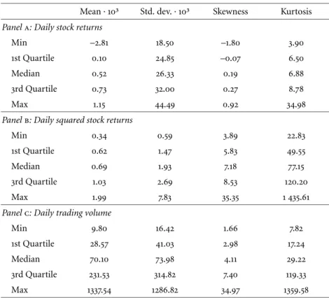
We start with some basic descriptive analysis of the time series of stock returns and trading volume. As can be seen from panelaof table1, the average daily stock return over the period under study ranges from – 0.28% (Netia) to0.12% (bre) with a median of –0.05%. Standard devi-ation is the lowest forpkn(1.85%) and the highest for Netia (4.45%).

The commonly reported fact of fat-tailed and highly-peaked return distributions is being supported by most of our series. The median of stock return kurtosis is6.88and ranges from34.98(sfc) to3.9(pkn). Return skewness is the highest for Netia (0.92) and the lowest forsfc (–1.8) with a median of 0.19. By applying Jarque-Bera and chi-square goodness-of-fit tests for normality, we additionally find strong support for the hypothesis that our return series do not come from a normal dis-tribution. Concerning autocorrelation properties, the Ljung-BoxQ-test statistics for the15th order autocorrelation provide evidence of signifi-cant low-order autocorrelation in about50% of all cases.

Unlike stock returns, both return volatility and trading volume com-monly display strong persistence in their time series. By means of Ljung-BoxQ(15)-statistics we find strong support for the hypothesis that trad-ing volume exhibits serial autocorrelation. Consistent with the stylized facts of volume series listed by Andersen (1996), our volume data exhibit a high degree of non-normality, expressed by their considerable kurtosis and their being skewed to the right (see panelcof table1).

As a proxy for return volatility we use the squared values of daily stock returns. These time series display the usual time dependency of stock returns in the second order moment (volatility persistence) implying, among other things, that returns cannot be assumed to be i. i. d. As for trading volume, the null hypothesis of squared returns coming from a normal distribution is strongly rejected (panelbin table1).

abnormal returns andabnormal trading volume One point that is essential in distinguishing our study from other contri-butions is that we focus on interactions between abnormal stock returns

table 1 Aggregated summary statistics for stock market data ofwig20companies Mean ·10³ Std. dev. ·10³ Skewness Kurtosis Panela: Daily stock returns

Min –2.81 18.50 –1.80 3.90

1st Quartile 0.10 24.85 –0.07 6.50

Median 0.52 26.33 0.19 6.88

3rd Quartile 0.73 32.00 0.27 8.78

Max 1.15 44.49 0.92 34.98

Panelb: Daily squared stock returns

Min 0.34 0.59 3.89 22.83

1st Quartile 0.62 1.47 5.83 49.55

Median 0.69 1.93 7.18 77.15

3rd Quartile 1.03 2.69 8.53 120.20

Max 1.99 7.83 35.35 1 435.61

Panelc: Daily trading volume

Min 9.80 16.42 1.66 7.82

1st Quartile 28.57 41.03 2.98 17.24

Median 70.10 73.98 4.11 29.22 3rd Quartile 231.53 314.82 7.40 119.33

Max 1337.54 1286.82 34.97 1359.58

and abnormal trading volume, instead of simple return and volume data. Since we concentrate on individual companies, instead of index data, our goal is to establish unique firm-specific relationships, i. e. we filter out systematic price and volume effects. For each trading daytwe compute the abnormal returnARi,t for companyi as the difference between the

actual ex-post return and the security’s normal (expected) return. For-mally we have

ARi,t =Ri,t−ERi,t|Ii,t−1 (1)

whereRi,tstands for the actual return of firmion dayt andE[Ri,t|It−1] stands for the predicted (normal) return conditional on the information setIt−1.

To model risk-adjusted expected returnsE[Ri,t|It−1]we use the Market Model approach, which relates a security’s return to the return of the market. The latter is approximated in our study by the log-returns of thewig, which comprises the majority of firms listed on the primary

market of the Warsaw Stock Exchange. For each day the relevant model parameters are estimated by means of an olsmethod. The estimation window comprises100trading days prior to that date. Since our analysis starts on January2,1995, this implies that the first realisation of abnormal stock returns for each company can be observed for the101st trading day in1995.

Abnormal trading volume is computed in a similar way. To isolate information-related trading activity, we follow Tkac (1999) who found that market-wide trading is also an important component of the trad-ing activity of individual firms, and that it should be taken into account when modeling volume time series. However, the application of a ‘Vol-ume Market Model’ proposed in Ajinkya and Jain (1989) generates many statistical problems. We find that the resulting abnormal volume series mostly depart from the underlying model assumptions. This leads to biased inferences. Taking this into account, we follow, among others, Beneish and Whaley (1996) by using firm-specific average volume data as a benchmark for normal trading volume. As was the case with the estimation window for the return parameters in the Market Model, the estimation window for the mean firm-specific volume also covers100 trading days.

testing for unit root

Testing for causal relationships between trading volume and stock price data can be sensitive to non-stationarities. Therefore, we check whether the time series of stock returns and trading volume can be assumed to be stationary by using the augmented Dickey-Fuller (adf) test. This is necessary to avoid model misspecifications and biased inferences. The adftest is based on the regression:

Δyt=μ+γyt−1+

p

i=1

δΔyt−i+εt, (2)

whereytstands for stock return or trading volume on dayt,μ,γ andδ

are model parameters, andεtrepresents a white noise variable. The unit

root test is carried out by testing the null hypothesis of a unit root in the stochastic process generatingyt(γ = 0)against the one-sided alternative

γ <0.

We conductadftests for each company’s time series of stock returns. We find the parameterγto be negative and statistically significant at rea-sonable levels in all cases. The same is true for the time series of trading

table 2 Cross-correlation coefficients between abnormal stock returns (AR), abnormal return volatility (AR2) and abnormal trading volume (AV)

j=−2 j=−1 j=0 j=1 j=2 Panela:Corr(ARt,AVt−j) Min –0.02 –0.01 0.04 –0.03 –0.02 1st Quartile 0.03 0.08 0.09 –0.01 –0.01 Median 0.04 0.10 0.12 0.00 0.00 3rd Quartile 0.07 0.13 0.13 0.03 0.02 Max 0.13 0.18 0.16 0.05 0.04 Panelb:Corr(AR2t,AVt−j) Min –0.10 –0.06 –0.07 –0.08 –0.13 1st Quartile 0.05 0.08 0.09 0.03 0.01 Median 0.08 0.15 0.17 0.07 0.04 3rd Quartile 0.11 0.20 0.20 0.10 0.07 Max 0.17 0.30 0.32 0.14 0.13

volume. Hence we come to the conclusion that both time series of stock returns and trading volume can be assumed to be invariant with respect to time.

cross-correlation analysis

At the beginning of our investigation of interactions between abnor-mal stock return and abnorabnor-mal trading volume data we calculate simple cross-correlation coefficientsCorrfor all companies:

Corr[ARt,AVt]= Cov[ARt,AVt]

SD[ARt]·SD[AVt], (3)

whereARt(AVt)denotes abnormal stock return (abnormal trading

vol-ume) on dayt,Covstands for covariance andSDis standard deviation. From panelaof table2we see that there is no direct contemporaneous correlation between abnormal stock return levels and excess trading vol-ume. The same results are obtained when one computesCorr between

ARand lagged (leading) data ofAV.

On the other hand, panelb of table2shows a positive contempora-neous correlation between abnormal trading volume and abnormal re-turn volatility. From this observation it follows that, due to its impact on return volatility, trading volume might indirectly contain information about stock price behaviour.

We also find an asymmetry in the cross correlation between squared

ARandAVaround zero. In all cases,Corr[AR2_t,AVt−j]is greater forj=−1

than forj = 1.This fact is in line with the widespread expectation that trading volume is, at least partly, induced by heavy price fluctuations.

4 Contemporaneous Relationship stock returns andtrading volume

In this section we test the contemporaneous relationship between ab-normal stock returns and excess trading volume. We use a multivariate simultaneous equation model proposed by Lee and Rui (2002), which is defined by the two equations:

ARt =α0+α1AVt+α2ARt₋1+ε1,t;

AVt=β0+β1ARt+β2AVt−1+β3AVt−2+ε2,t. (4)

We assume εt to be white noise. One has to take into account that

the jointly determined endogenous variables in each equation are not independent of the disturbances. This is important in respect to the esti-mation process. To take this possible dependence into account, we apply Full-Information Maximum Likelihood (fiml) methodology.fiml gen-erates asymptotically efficient estimators. An additional advantage is that the cross-equation correlations of the error terms are taken into account (see e. g. Davidson and MacKinnon2003). The significance of all coeffi -cients in models (4), (5) and (6) (see below), is proved by means of the t-Student test (t-ratio coefficients).

The findings are in line with our expectations of almost no essential contemporaneous relationship between abnormal stock returns and ex-cess trading volume. Across the whole sample, the parametersα1andβ1 in (4) turn out to be statistically significant in only4cases. Since the ma-jority of our abnormal return series exhibit no serial correlation, we find parameterα2to be significant in only6cases.

Time dependence in the trading volume time series is supported by the highly significant values found for parametersβ2 (16cases) and β3 (11cases). As one would expect, the sign of these coefficients is positive in all but two cases, implying positive autocorrelation in volume data.

Even though we find abnormal stock return levels and trading volume to be mutually independent, this does not mean that no relationships can be found in these market data at all. Several authors report that price fluctuations tend to increase in face of high trading volume. Therefore,

a relation might exist between higher order moments of excess stock re-turns and trading volume.

In addition, we check whether this volatility-volume relationship is the same irrespective of the direction of the price change, or whether trading volume is predominantly accompanied by either a large rise or a large fall in stock prices. We test this by using a bivariate regression model, given by the following equation:

AVt=α0+φ1AVt−1+φ2AVt−2+α1AR2t +α2DtAR2t +εt. (5)

In model (5),Dt denotes a dummy variable that equals 1 if the

cor-responding abnormal returnARt is negative, and 0 otherwise. The

esti-mator of parameterα1measures the relation between abnormal return volatility and excess trading volume, irrespective of the direction of the price change. The estimator ofα2, however, reflects the degree of asym-metry in this relationship. To avoid the problem of serially correlated residuals, we include lagged values ofAV up to lag2. After this, we find the error termεtin equation (5) to be largely serially uncorrelated.

By means of the mlmethod we estimate equation (5). According to our computations, the estimate of parameterφ1is significant in17cases and the estimate of parameterφ2is significant in15cases. We also estab-lish that parameterα1is positive and significant for all but2companies. This is in line with our earlier hypothesis of a strong contemporaneous relationship between squaredARandAV. The estimate of parameterα2 is significant in13cases and negative in all of these. We find that for our sample of the Warsaw Stock Exchange, strong price changes are always accompanied by an increase in trading volume, irrespective of the direc-tion of price fluctuadirec-tions.

trading volume and volatility

The stochastic process of stock returns is given by means of an aug-mented Market Model with an autoregressive term of order 1 in the conditional mean equation below. The conditional variance is captured by an adapted gjr-garch(1,1) model (Glosten et al.1993). In this ver-sion, trading volume is included as an additional predetermined regres-sor. Thegjrmodel captures the asymmetric (leverage) effect discovered by Black (1976), which states that bad information, reflected in an un-expected decrease in prices, causes volatility to increase more than good news. Engle and Ng (1993) supplied a theoretical and empirical support and stated that, among alternative models of time-varying volatility, the gjrmodel is the best at efficiently capturing this effect.

The model is represented by the following two equations: Rt =α0+α1Rt−1+α2Rm,t+εt, εt ∼(0,σ2t);

σ2

t =ht =β0+β1ht−1+β2ε2t−1+β3S−t−1εt2−1+γVt. (6)

Hereεt is assumed to be distributed ast-Student with νdegrees of

freedom conditional on the set of information available att−1;σ2_t repre-sents the conditional variance ofεt; andS−_t−1is a dummy variable, which

takes the value of 1 in the case of the innovationεt−1being positive and 0 otherwise. Model (6) rests upon the assumption that trading volume is a proxy for the flow of information into the market: if return volatility is in fact mostly influenced by the information flow, the effect of volatil-ity clustering should decrease if one incorporates trading volume in the conditional variance equation. In (6) the sum of parametersβ1 andβ2 reflects the persistence in the variance of the unexpected returnεt,

tak-ing values between 0 and 1. The closer this sum is to unity, the greater the persistence of shocks to volatility (volatility clustering). The estimate of parameterβ3 accounts for potential asymmetries in the relationship between return innovation and volatility.

We apply at-Student distribution for the return innovations εt

be-cause we find this to fit our turnover ratio series best. Thus, we use the conditionalt-Student distribution for which the normal is a special case (ν >30). For model (6), a likelihood functionLis defined as:

L=T lnΓ _ν+1 2 −lnΓ _ν 2 − 1 2ln[π(ν−2)] −1 2 t t=1 ln(σ2t)+(1+ν)ln 1+ 1 ν−2 εt σ2 t , (7)

whereTdenotes the sample size andΓ(.)denotes the gamma function. The model parameters are estimated by means of themlmethod. As a first step, we estimate the parameters of model (6) assuming thatγis equal to 0 (restricted variance equation, see table 3). We find that the estimate of parameterβ1as well as the estimate of parameterβ2is signif-icant in nearly all cases. For14companies, the observed sum (β1+β2) lies within the range[0.9−1]. The average is0.93, which indicates high per-sistence in conditional volatility. In most cases,β3is positive, but turns out to be statistically significant for one company only. This indicates that the asymmetric reaction of conditional variance to return innova-tions is rather modest in our data. In the next step we are interested in the unrestricted equation for conditional variance. We find parameterγ

table 3 Persistence in conditional stock return volatility [restricted versus unrestricted version of model (6)]

Symbol (β1+β2)a (β1+β2)b Symbol (β1+β2)a (β1+β2)b ago 0.93 0.08 kty 1.00 0.03 bph 0.98 0.97 net 1.00 0.88 bre 0.95 0.13 orb 0.97 0.21 bzw 0.81 0.90 peo 0.87 0.91 cpl 0.99 0.08 pkm 0.96 0.06 cst 0.75 0.41 pkn 0.96 0.89 dbc 0.70 0.11 sft 0.91 0.04 fsc 0.96 0.37 stx 0.96 0.89 kgh 0.98 0.89 tps 0.98 0.83 Average 0.93 0.48 to be positive and highly significant across the whole sample. Our data show a considerable decrease in the persistence of volatility when trad-ing volume is included in (6). The sum of parametersβ1andβ2declines for almost all companies. The mean falls from 0.93 to 0.48. The esti-mate of parameterβ2shows a significant drop. In the unrestricted form it becomes, for the most part, insignificant. Table3gives the degree of persistence in variance, measured by the sum (β1+β2) for the restricted and unrestricted form of (6). Results are shown for all stocks under con-sideration.

It cannot be derived from our data that trading volume is the true source of persistence in volatility. Empirical results support the conjec-ture that trading volume might itself be partly determined by return volatility, causing a simultaneity bias in the coefficient estimates. To solve this simultaneity problem we re-run model (6) substitutingVt−1forVt.

In line with Gallo and Pacini (2000), we find that volatility persistence under this approach remains almost the same as in the restricted version of (6). It can be concluded that contemporaneous trading volume is a sufficient statistic for the history of return volatility. Despite this, our re-sults can only partly be interpreted as an indication that themdhholds true.

5 Dynamic Relationship

Up to this point, our investigations focused exclusively on contempo-raneous relationships between trading volume and stock returns, and

trading volume and return volatility. The following part of the paper studies dynamic (causal) interactions between these variables. Testing for causality is important because it permits a better understanding of the dynamics of stock markets, and may also have implications for other markets.

From section3we get a hint that it is probable that causality is present in the relationship between return volatility and trading volume. This hypothesis can be proved by means of the Granger causality test (Granger 1969). A variableY is said not to Granger-cause a variableX if the dis-tribution ofX, conditional on past values ofX alone, equals the distri-bution ofX, conditional on past realizations of both X and Y. If this equality does not hold,Y is said to Granger-causeX. This is denoted by Y G. c.→ X. Granger causality does not mean thatY causesX in the more common sense of the term, but only indicates thatY precedesX. In the case of the feedback relationship (i. e.XGranger-causesYand vice versa) this relation is written asY G. c.↔ X.

As a test of Granger causality, we apply a bivariate vector autoregres-sion (var) of the form:

ARt =μ1+ p i=1 α1,iARt₋i+ p i=1 β1,iAVt₋i+ε1,t; AVt=μ2+ p i=1 α2,iAVt−i+ p i=1 β2,iARt−i+ε2,t. (8)

Model (8) is estimated using anolsmethod. In order to choose an appropriate autoregressive lag lengthpof the var, we apply the Akaike information criterion (aic). Based on this measure of goodness-of-fit, we establish the proper lag lengthpto be equal to 2 for all companies.

In terms of the Granger causality concept, it is said thatAR(AV) does not Granger-causeAV (AR) if the coefficientsβi (i = 1, . . . , p) in (8),

respectively, are not significant, i. e. the null hypothesisH0:β1 = β2 =

. . .=βp=0 cannot be rejected.

To test the null, we calculate theF-statistic: F = SSE0−SSE

SSE ·

N−2p−1

p . (9)

In (9) SSE0 denotes the sum of squared residuals of the regression model constrained byβi = 0(i = 1, . . . , p),SSE is the sum of squared

residuals of the unrestricted equation, andN stands for the number of observations. The statistic (9) is asymptoticallyF distributed under the

table 4 Number of rejected null hypotheses based on the Granger causality test Panela:Causality between excess trading volume and abnormal stock returns

ARG. c.→AV AVG. c.→AR ARG. c.↔AV

Sample size:18companies 11 0 1 Panelb:Causality between excess trading volume and squared abnormal stock returns

AR2G. c._{→AV AV}G. c._→AR2 _AR2G. c._↔AV

Sample size:18companies 8 1 3 Level of significance is5%. Orderpin (8) is equal to2.

non-causality assumption, withpdegrees of freedom in the numerator and(N−2p−1)degrees of freedom in the denominator.

Concentrating on the rejection of the null hypothesis of Granger non-causality, panelaof table4demonstrates that abnormal returns (excess trading volume) precede excess trading volume (abnormal returns) in 11(0) cases. Both numbers reflect exclusively unidirectional causalities. Only in one case a two-way causality (feedback relation) is detected. To conclude, short-run forecasts of current or future stock returns in gen-eral cannot be improved by the knowledge of recent trading volume data. The observation that stock returns precede trading volume in approxi-mately half of all cases is in line with similar findings by Glaser and Weber (2004) and confirms predictions from overconfidence models. To sum-marize, we find only weak evidence of causality between abnormal stock returns and excess trading volume, especially causality running from trading volume to stock returns. This is in line with our expectations.

To evaluate dynamic relationships between stock return volatility and trading volume, we substitute the abnormal return level for the squared values of abnormal stock returns, and re-estimate the model (8). Panel b of table4confirms the existence of causal relationships fromAR2to

AV. In 10cases,AR2 precedesAV, whereas in only 1case does Granger causality run fromAVtoAR2. This result is again in line with our earlier finding that stock price changes in any direction have information con-tent for upcoming trading activities. The preceding return volatility can also be seen as some evidence that the arrival of new information might follow a sequential rather than a simultaneous process.

Our results indicate that data on trading activity have only little addi-tional explanatory power for subsequent price changes that is indepen-dent of the price series. In this sense, our empirical results for the Polish stock market does not overall corroborate theoretical suggestions made by Blume et al. (1994) and more recently by Suominen (2001).

6 Conclusions

Our paper presents a joint dynamics study of daily trading volume and stock returns for Polish companies listed in thewig20. We test whether volume data provide only a description of trading activities or whether they convey unique information that can be exploited for modeling stock returns or return volatilities. These relationships are investigated by the use of abnormal stock return and excess trading volume data. Our re-sults give no evidence of a contemporaneous relationship between mar-ket adjusted stock returns and mean adjusted trading volume. The lin-ear Granger causality test of dynamic relationships between these data does not indicate substantial causality. We can conclude that short-run forecasts of current or future stock returns cannot be improved by the knowledge of recent volume data and vice versa. This finding is in line with the efficient capital market hypothesis. However, the Polish data show extensive interactions between trading volume and stock price fluc-appendix a Companies included in the sample, symbol legend

and period of quotation*

plpkn0000018 20April1999–29April1999 plpekao00016 7February1995–29April2005 pltlkpl00017 2January1995–29April2005 plkghm000017 2January1995–29April2005 plbph0000019 27October1995–29April2005 plagora00067 25May1998–29April2005 plbz00000044 2January1995–29April2005 plprokm00013 22April1997–17February2005 plnetia00014 10July1997–29April2005 plbre0000012 30January1996–29April2005 plstlex00019 11July2000–29April2005 plkety000011 20November1997–29April2005 plorbis00014 30June1998–29April2005 plsoftb00016 10February1998–29April2005 plcmpld00016 26November1999–29April2005 plcrsnt00011 2June1998–29April2005 plcelza00018 2January1995–29April2005 pldebca00016 18November1998–29April2005

tuations. We find that squared abnormal stock returns and excess trad-ing volume are contemporaneously related. This implies that both time series might be driven by the same underlying process. In contrast to Brailsford (1996), our findings provide evidence that for the Polish stock market this volatility-volume relationship is independent of the direc-tion of the observed price change. We apply our investigadirec-tions to a con-ditional asymmetric volatility framework in which trading volume serves as a proxy for the rate of information arrival on the market. The results to some extent support suggestions of the Mixture of Distribution Hy-pothesis, i. e. thatarchis a manifestation of daily time dependence in the rate of new information arrival. We also detect dynamic relationships between return volatility and trading volume data.

References

Ajinkya, B. B., and P. C. Jain.1989. The behavior of daily stock market trading volume.Journal of Accounting and Economics11:331–59. Andersen, T. G. 1996. Return volatility and trading volume: An

infor-mation flow interpretation of stochastic volatility.Journal of Finance 51:169–204.

Avouyi-Dovi, S., and E. Jondeau.2000. International transmission and volume effects ing5stock market returns and volatility.bis Confer-ence Papers, no.8:159–74.

Beneish, M. D., and R. E. Whaley.1996. An anatomy of thes&p game. Journal of Finance51:1909–30.

Bessembinder, H., and P. J. Seguin.1993. Price volatility, trading volume and market depth: Evidence from futures markets.Journal of Financial and Quantitative Analysis28:21–39.

Black, F.1976. Studies in stock price volatility changes. InProceedings of the 1976Business Meeting of the Business and Economics Statistics Section, 177–181. N. p.: American Statistical Association.

Blume, L., D. Easley, and M. O’Hara.1994. Market statistics and technical analysis: The role of volume.Journal of Finance49:153–81.

Brailsford, T. J.1996. The empirical relationship between trading volume, returns and volatility.Accounting and Finance35:89–111.

Brock, W. A., and B. D. LeBaron.1996. A dynamic structural model for stock return volatility and trading volume.The Review of Economics and Statistics78:94–110.

Clark, P. K.1973. A subordinated stochastic process model with finite vari-ance for speculative prices.Econometrica41:135–55.

Copeland, T.1976. A model of asset trading under the assumption of se-quential information arrival.Journal of Finance31:135–55.

Darrat, A. F., S. Rahman, and M. Zhong.2003. Intraday trading volume and return volatility of thedjiastocks: A note.Journal of Banking and Finance27:2035–43.

Davidson, R., and J. G. MacKinnon.2003.Econometric theory and meth-ods.New York: Oxford University Press.

Engle, R. F., and V. K. Ng.1993. Measuring and testing the impact of news on volatility.Journal of Finance48:1749–78.

Epps, T. W., and M. L. Epps.1976. The stochastic dependence of security price changes and transaction volumes: Implications for the mixture-of-distribution hypothesis.Econometrica44:305–21.

Gallo, G. M., and B. Pacini.2000. The effects of trading activity on market volatility.The European Journal of Finance6:163–75.

Glaser, M., and M. Weber.2004. Which past returns affect trading volume? Working Paper, University of Mannheim.

Glosten, L. R., R. Jagannathan, and D. E. Runkle.1993. On the relation between the expected value and the volatility of the nominal excess return on stocks.Journal of Finance48:1779–801.

Granger, C.1969. Investigating causal relations by economic models and cross-spectral methods.Econometrica37:424–38.

Hiemstra, C., and J. D. Jones. 1994. Testing for linear and nonlinear Granger causality in the stock price–volume relation. Journal of Fi-nance49:1639–64.

Karpoff, J. M. 1987. The relation between price changes and trading volume: A survey. Journal of Financial and Quantitative Analysis 22:109–26.

Lamoureux, C. G., and W. D. Lastrapes.1990. Heteroscedasticity in stock return data: Volume versusgarcheffects.Journal of Finance45:221–9. Lamoureux, C. G., and W. D. Lastrapes.1994. Endogenous trading vol-ume and momentum in stock-return volatility.Journal of Business and Economic Statistics12:253–60.

Lee, B.-S., and O. M. Rui.2002. The dynamic relationship between stock returns and trading volume: Domestic and cross-country evidence. Journal of Banking and Finance26:51–78.

Omran, M. F., and E. McKenzie.2000. Heteroscedasticity in stock returns data revisited: Volume versusgarcheffects.Applied Financial Eco-nomics10:553–60.

Suominen, M.2001. Trading volume and information revelation in stock markets.Journal of Financial and Quantitative Analysis36:545–65. Tauchen, G., and M. Pitts.1983. The price variability-volume relationship

on speculative markets.Econometrica51:485–505.

Tkac, P. A.1999. A trading volume benchmark: Theory and evidence. Jour-nal of Financial and Quantitative AJour-nalysis34:89–114.