Compendium of branched broomrape
research
Section 6. Life cycle
A COMPILATION OF RESEARCH REPORTS FROM THE
BRANCHED BROOMRAPE ERADICATION PROGRAM SOUTH
AUSTRALIA
Compendium of branched broomrape research
Information current as of 4 December 2013 © Government of South Australia 2013
Disclaimer
PIRSA and its employees do not warrant or make any representation regarding the use, or results of the use, of the information contained herein as regards to its correctness, accuracy, reliability and currency or otherwise. PIRSA and its employees expressly disclaim all liability or responsibility to any person using the information or advice.
Table of Contents
1. Effect of seed density on probability of branched broomrape establishment 4
2. Growing degree days 7
3. Relationship between infected broomrape paddocks and seasonal growing conditions - Analysis 1 17 4. Paddock level broomrape infection in relation to seasonal conditions - Analysis 2 25 See also the following publication:
Prider J., Williams A. (2014) The reproductive biology and phenology of the introduced root holoparasite, Orobanche ramosa subsp. mutelii (branched broomrape in South Australia (in preparation)
1.
Effect of seed density on probability of branched
broomrape establishment
Ray Correll
CSIRO Mathematics
February 2003
Abstract
The probability of establishment of branched broomrape is shown to be approximately proportional to the number of seeds released.
The only assumptions required in deducing the above are that the likelihood of establishment is low and that the seeds are scattered.
Consideration is given to the case when the seeds remain clumped the likelihood of establishment is less – in such cases the likelihood would be proportional to the number of clusters.
Introduction
The release of a paddock from quarantine that has been imposed because of an infection of branched broomrape will require a guarantee that that paddock contains no branched broomrape plants or viable seed. Sampling cannot guarantee that there are no seeds in that paddock. Release of paddocks from quarantine must be on a risk basis – a paddock is released only when the risk of spread from that paddock is sufficiently low.
As well as attempting to release paddocks from quarantine, the branched broomrape program is endeavoring to contain existing infections within a quarantine zone. Various ways are being used to restrict the spread. These include stringent restrictions on the movement of farm machinery and feed. There is also the possibility of stock spreading the disease through ingestion of the seeds and subsequent excretion of the seeds in a viable state.
The probability of seed survival will depend on many factors, including the animal type, nutrient levels and the rate of progress of the seed through the gut. The managers of the branched broomrape program are interested in the effect of increasing seed density of broomrape on its probability of successful
establishment after passing though the gut of an animal (e.g.. sheep or rabbit).
The probability of a seed surviving through the gut is small, but must be considered. This paper deals with the effect of seed density on the probability of a new infestation being caused by seeds that have passed through the gut.
Biological assumptions
It is assumed that a foraging animal (e.g. sheep or rabbit) can eat seeds of broomrape. A small proportion p of these seeds survives the gut and persists in a location such that it has the potential to flourish into a mature plant. There are several possibilities of how this may occur. We consider two extremes –
1. The seeds that are eaten behave independently;
2. The seeds remain clumped (perhaps remaining inside a capsule) up to the time of germination. We will refer to these as the independent and clumped cases.
Estimation of probabilities
Independent case
The probability of a seed being successful (surviving the gut and being lodged near an appropriate host) we defined above as p.
The probability of it not being successful is therefore (1 - p). The probability of two seeds both being unsuccessful is then (1 – p) (1 – p).
This generalizes to the probability of n seeds all being unsuccessful to (1 – p)n.
The probability of at least one being successful then is P(success) = 1 – (1 – p)n
For low seed density, the probability of successful establishment is proportional to the seed density. Details are given in the section Mathematical Considerations.
For a situation where there is a high probability of a success, the above approximation is not quite correct. However you will have lots of branched broomrape, so will not be interested in whether you have 90 or 100 successful establishments will be largely immaterial for plant quarantine (phytosanitary) purposes. In the hypothetical situation that a sheep eats a ripe indehisced capsule of seeds, it is feasible that all the seeds will stay together in their journey through the alimentary canal, and could come out in a single pellet. In that case, it is important where the capsule lands. If one seed is successful, then most of the other seeds could have been successful also. The probability of establishment in that case would be proportional to the number of capsules rather than the number of seeds.
Clumped case
In this situation, it is assumed that the seeds remain clumped together (perhaps inside the seed capsule) and are excreted in a single pellet. In that situation, if one seed has conditions that are favourable, then it is likely that all seeds will have favourable conditions. The success depends on the factors that affect the whole capsule rather than the individual seeds.
It is conceivable that if there is a clump of seeds and only a single available host plant, the probability of success will be governed by the availability of hosts, and seeds from a capsule that lodges in a favourable environment may compete with each other.
At a broader level, even if the seeds remain within a capsule, the individual capsules will behave more or less independently.
The likelihood of establishment in the clumped case will be reduced (perhaps by a factor somewhat less than the number of seeds in a cluster). In such a case, the likelihood of establishment will be determined more by the number of clusters than the number of seeds per cluster.
Mathematical Considerations
We consider the formulaFor ease of notation we use P to indicate P (success). We expand (1 – p)nas a binomial to give
1 – np + n(n –1 )/2p2 – n(n – 1)(n – 2)/6p3 …..
When the probability of successful establishment is low (np <<n), the above series can be estimated by the first two terms, namely 1 – np.
An estimate of successful establishment is therefore P = P(success) ≈ 1 – (1 – np) = np.
For small p, where np << 1, the probability of successful establishment is directly proportional to the number of seeds provided that they are randomly distributed (or well mixed in the gut).
An alternative derivation can be to consider the rate of change of P as n changes. Differentiating P with respect to n gives
np
p
dn
dP
ln
1
1
We note that ln
1 p
p, hence (and also using the approximate binomial expansion) we can write
np
p
dn
dP
1
and as (1-np) is approximately 1 for small np <<1, the rate of change of probability P as n increases is directly proportional to p, and almost unaffected by n. It follows therefore that P is directly proportional to n.
2.
Growing degree days
Anna Williams and Jane Prider
Branched Broomrape Eradication Program
February 2013
Introduction
Key limitations for the control of broomrape are finding it, knowing when to look for plants at various developmental stages, and when to apply herbicides, given that herbicides are the key method to prevent emergence after attachments have occurred. This requires knowledge of timing of germination,
underground development, attachment and emergence.
Growing Degree Days (GDD) are used to determine development rates such as flowering time of plants and also in determining opportune timing for application of chemicals for disease and pest control. They are typically counted from average daily soil temperatures and accumulate over the growing season or the time period of interest.
GDD have been used to predict the growth development of Orobanche minor on red clover hosts (Eizenberg et al. 2004, Eizenberg et al. 2005). GDD have also been used to predict O. cumana and Phelipanche aegyptiaca development on sunflower hosts (Eizenberg et al. 2009, Ephrath and Eizenberg 2010, Eizenberg et al. 2012) and P. aegyptiaca infection of tomato (Ephrath et al. 2012). This information has been used in selection of the optimal timing for herbicide applications for O. minor and O. cumana control (Eizenberg et al. 2006, Eizenberg et al. 2012).
In the Quarantine Area, broomrape emergence occurs between July and December. Discovery surveys commence only after the first emerged plants have been found. Out of season emergence has been observed in summer on weeds in irrigated crops.
Given the wide potential window of emergence there is a need to understand the developmental cycle. A study was initiated in 2006 to evaluate the timing of attachments and emergence in O. ramosa in relation to soil temperature.
Methods
Glasshouse study 2006
Carrot and cretan weed hosts were planted in 0.8 L pots of sand inoculated with broomrape seed. Pots were prepared by mixing 0.01 g of broomrape seed per pot of Tailem Bend sand. Four host seeds were sown in each pot and later thinned to one host per pot. Hosts were sown on two planting dates, 5 weeks apart, in August and September 2006. Hosts were also planted in November 2006 but a limited number of samples were collected from these plants. 10 pots of each host without broomrape seed were controls. Plants were kept in a glasshouse. Soil temperature was recorded with a T-Tech Temperature Logger, recording temperature every 1 minute and recording the hourly average. The daily minimum and maximum soil temperature commencing from the host sowing date were converted to Growing Degree Days (GDD) units using the formula:
Seven pots of broomrape infested hosts from each planting date were randomly selected every 100 GDD, soil was removed, and the roots were washed. Broomrape attachments were counted and measured on each host plant under a microscope. The controls were collected on the final retrieval date.
At harvest the following variables were measured:
• Host leaf length
• Number of host leaves
• Number of host flowers
• Diameter of base of host stem
• Length of host tap root
• Number of broomrape plants
• Broomrape developmental stage
• Parasite and host dry weight Broomrape developmental stages were:
1. New attachments: tubercle less than 2 mm in diameter, germ tube typically still present 2. Small attachments: tubercle up to 5 mm in diameter
3. Large attachments: tubercle more than 5 mm in diameter 4. Emerged plants
Field study 2006
Cretan weed volunteer hosts were sampled at the Mannum Trial Site in 2006. 300 cretan weed plants of similar size were selected and tagged with a pin marker soon after establishment. Every week, 10 X 30 cm soil cores, 15 cm deep, centred on each marked plant were collected and the soil washed from the roots. Roots were later examined under a microscope. Host and parasite data were collected as for the glasshouse study.
In addition, the broomrape was also divided into the following developmental stages to enable comparisons with other published studies:
1. New attachments (as above)
2. Tubercles with roots: tubercles larger than 2 mm in diameter with roots
3. Tubercles with buds: tubercles with roots (or in some cases the roots may have dropped off) with a bud shoot less than 10 mm long
4. Tubercles with stems: tubercles with roots (or in some cases the roots may have dropped off) with a stem greater than 10 mm long
5. Emerged plants
Minimum and maximum soil temperature data were accessed from the nearest weather station at Mypolonga for the calculation of Growing Degree Days (GDD). Temperatures were converted to GDD units using Formula 1. The starting date for the calculation of GDD was the first rains of the season that resulted in the germination of hosts.
Field study 2007
Broomrape plants were collected from volunteer hosts at two sites using the same method as in 2006. Cretan weed hosts were sampled from the Mannum trial site and capeweed hosts from a site at Wynarka. Soil temperature data was collected from weather stations located at each of these sites. GDD were calculated using equation 1 from the first rains of the season.
Results
Glasshouse experiment 2006
For planting dates in August and September, broomrape plants were first found attached to cretan weed and carrot hosts 35 days after host seeds were sown. For hosts sown in November, attachments were found at 28 days. The accumulation of GDD occurred slower at the earlier sowing dates such that attachments started appearing at 742, 700 and 580 GDD respectively for cretan weed (Fig. 1A) and 750, 690 and 440 GDD for carrot (Fig. 1B).
Figure 1. Number of broomrape plants at different stages of development on A) cretan weed hosts and B) carrot hosts, in relationship to cumulative GDD. PD1 = August sowing, PD2 = September sowing, PD3 = November sowing. Each point is the average of 7 host plants (n = 7). For clarity, zero values are not shown for GDD before the first appearance of that tubercle size stage.
0 0.1 0.2 0.3 0.4 0.5 0.6 0.7 0.8 0.9 1 0 500 1000 1500 2000 2500 lo g 10 num ber o f br o o m rap e pl an ts per ho st GDD 0 0.2 0.4 0.6 0.8 1 1.2 1.4 1.6 0 500 1000 1500 2000 2500 lo g 10 num ber o f br o o m rap e pl an ts per ho st GDD
New attachments PD1 New attachments PD2
New attachments PD3 Emerged PD1
Small attachments PD1 Small attachments PD2
Large attachments PD1 Large attachments PD2
A
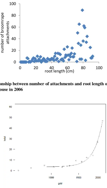
Figure 2. Relationship between number of attachments and root length of cretan weeds hosts grown in pots in glasshouse in 2006
Figure 3. Weibull four-parameter model fitted to data for total number of broomrape plants on cretan weed hosts grown in the glasshouse in 2006. Each point is the average of 7 plants.
Figure 4. Proportion of broomrape plants in different size categories at each sampling date on cretan weed hosts planted in pots in August 2006.
0 20 40 60 80 100 0 20 40 60 80 100 num ber o f br o o m rap e at ta chm ents root length (cm) 0 10 20 30 40 50 60 70 80 90 100 7 14 21 28 35 42 49 56 63 70 77 84 91 98 105 112 p ro p o rt io n o f b ro o m ra p e p la n ts
Days after planting
Flowering Budding Emerged but no buds Extra large attachments (=>30.1mm) Large attachments (10.1mm - 30mm) Immature attachments (2.1mm - 10mm) New attachments (<= 2mm)
There was a positive relationship between host root length and the number of new attachments (Fig. 2). Roots less than 10 cm long did not support any attachments. Roots grew to this length earlier in the November plantings.
Large attachments were found 42 days (900 GDD) after cretan weed hosts were sown in August. There was an exponential increase in the number of small and large tubercles on cretan weed hosts between 800 and 2000 GDD. The first cretan weed plant emerged at 1440 GDD. Overall the infection process of cretan weed by broomrape could be fitted to a Weibull four-parameter model (Fig. 3) Tubercle
development of broomrape on carrot hosts was slower than on cretan weed. Tubercles were not found until after 1000 GDD and the first plant emerged at 1560 GDD (Fig. 1B). Only a small proportion of
broomrape had emerged by the termination of sampling at 2270 GDD or 112 days after the August sowing. Sampling did not extend beyond 1500 GDD for the other sowing dates.
The proportion of new attachments on cretan weed increased gradually over time however the proportion of new attachments declined as tubercles developed so that by the time of the first emergence new attachments comprised half of the broomrape plants on each host (Fig. 4).
2006 Mannum Field Trial
The break of the season in Mannum occurred on March 27th in 2006 with a fall of over 30 mm in two days (Fig. 5). This resulted in the germination of the target host, cretan weed. Low rainfall occurred throughout the remainder of the growing season. Soil temperatures did not rise above 25 °C until the beginning of October. Minimum soil temperatures were approximately 10 °C although there were some very low temperatures in early May.
The first sampling of broomrape plants occurred in mid May. New attachments and small tubercles with roots were found on this date (Fig. 6). Small tubercles had formed by 730 GDD so these plants became attached before this. Larger tubercles with stems appeared after 750 GDD whilst emerged plants began appearing after 1500 GDD. The number of tubercles present per host plant was at its highest from 1000 to 1500 GDD and decreased after broomrape began emerging. Tubercle number showed no obvious correlation to rainfall (Fig. 6). However, the decrease in broomrape during September may have been a result of the low rainfall during August. The first emerged plant occurred on August 16th or at 1596 GDD.
New attachments continued to be found until the first emerged plant occurred (Fig. 7). Only dead new attachments were found after this date. Young tubercles with roots were found throughout the growing season in approximately equal proportion to young tubercles with bud shoots to less than 10 mm long. Larger tubercles with developing stems (> 10 mm long) began to appear from mid-June or 960 GDD.
Figure 5. Rainfall and soil temperatures throughout the 2006 growing season. Rainfall data are from the nearest weather station at Mannum (Bureau of meteorology). Soil temperature data are
0 5 10 15 20 25 30 -10 -5 0 5 10 15 20 25 30 35 40 rai nf al l ( m m ) so il tem per at ur e (° C)
minimum soil temperature maximum soil temperature daily rainfall
Figure 6. Average attachments per cretan weed host plant at different stages of development from soil cores collected at the Mannum Trial Site in 2006. The Growing Degree Days model is shown by the line.
Figure 7. Proportion of broomrape plants at different stages of development retrieved from 10 soil cores sampled at weekly intervals at the Mannum Trial Site in 2006.
0 500 1000 1500 2000 2500 3000 3500 0 2 4 6 8 10 12 14 1 -A pr -06 11 -A pr -06 21 -A pr -06 1 -M ay -06 11 -M ay -06 21 -M ay -06 31 -M ay -06 10 -J un -06 20 -J un -06 30 -J un -06 10 -J ul -06 20 -J ul -06 30 -J ul -06 9 -A u g -06 19 -A ug -06 29 -A ug -06 8 -S e p -06 18 -S ep -06 28 -S ep -06 8 -O c t-06 18 -O c t-06 28 -O c t-06 7 -Nov -06 17 -Nov -06 27 -Nov -06 G DD Num be r of at ta c hm en ts or r ai nf al l ( m m ) Date of collection
Small attachments group Murray Bridge Daily Rainfall (mm)
Large attachments group Emerged attachments
GDD accumulated from 27/3/06 0 0.1 0.2 0.3 0.4 0.5 0.6 0.7 0.8 0.9 1 17 -May 24 -May 31 -May 7-Jun 14-J un 21 -J un 28 -J un 5-Jul 12 -J ul 19 -J ul 26 -J ul 2 -A ug 9 -A ug 16 -A ug 23 -A ug 30 -A ug 6 -S ep 13 -S e p 20 -S e p 27 -S e p 4-O ct 11 -Oct 18 -Oct 25 -Oct 1 -Nov pr o po rti o n o f pl an ts in sta ge sampling date emerged underground stems tubercles with buds tubercles with roots new attachments
Field studies 2007
In the 2007 season, breaking rains occurred on April 29th and rainfall was very low through the growing
season, particularly at the more northern Mannum site. The first broomrape attachments at Wynarka were sampled on June 22nd at 720 GDD (Fig. 8). The first attachments at Mannum were observed on June 12th
at 600 GDD (Fig. 9). The first emergence was sampled at Wynarka on August 31st at 1510 GDD. The first
emergence at Mannum was sampled on September 19th at 1730 GDD.
Figure 8. Accumulated GDD and presence of broomrape attachments at the Wynarka site
Figure 9. Accumulated GDD and presence of broomrape attachments at the Mannum site. The 0 500 1000 1500 2000 2500 0 10 20 30 40 50 16 -Apr -07 30 -Apr -07 14 -M ay -07 28 -M ay -07 11 -J un -07 25 -J un -07 9 -J ul -07 23 -J ul -07 6 -Aug -07 20 -Aug -07 3 -Sep -07 17 -Sep -07 1 -Oc t-07 GD D
Rai
n
fal
l (
mm)
Date of collection
Broomrape attachments present Daily rainfall
GDD accumulation from 1st May 2007
0 500 1000 1500 2000 2500 0 10 20 30 40 50 19 -M ar -07 29 -M ar -07 8-A p r-07 18 -A p r-07 28 -A p r-07 8-M ay -07 18 -M ay -07 28 -M ay -07 7-Ju n -07 17 -J u n -07 27 -J u n -07 7-Ju l-07 17 -J u l-07 27 -J u l-07 6-A u g-07 16 -A u g-07 26 -A u g-07 5-Se p -07 15 -Sep -07 25 -Sep -07 5-Oct -07 15 -Oct -07
GDD
Rai n fal l (m m )Date of collection
Broomrape attachments present Daily rainfall
GDD accumulation from 1st May 2007
Figure 10. Average number of broomrape attachments per core found on sampled host plants on different dates at two sites.
Figure 11. Percentage of host plants in flower at the two field sites in 2006 and 2007 in relation to growing degree days.
There were more broomrape plants at the Mannum site than the Wynarka site (Fig. 10). The peak in broomrape numbers occurred during August at the Mannum site between 1000 and 1500 GDD. With the exception of root development (see Fig. 2), there were no obvious relationships between host development and broomrape development. For example, peak flowering of cretan weed hosts occurred earlier in 2006 than in 2007 but broomrape emergence and flowering occurred at similar times in both years (Fig. 11). Cretan weed host plants were much smaller in 2007 than in 2006 (data not shown).
0 0.5 1 1.5 2 2.5 3 3.5 4 4.5 18 -May -07 7 -J un -07 27 -J un -07 17 -J ul -07 6 -A ug -07 26 -A ug -07 15 -S ep -07 5-Oct -07 25 -Oct -07 br o o m rap e at ta chm ents sampling date Mannum Wynarka 0 10 20 30 40 50 60 70 80 90 100 0 500 1000 1500 2000 2500 % o f h o s t p la n ts i n f lo w e r GDD Mannum 2006 Mannum 2007 Schulz 2007
Discussion
We measured a consistent relationship between soil temperature and broomrape development. This was also relatively consistent between the hosts, cretan weed and carrot, and in field and glasshouse conditions. Under the cooler temperatures that may be expected during the growing season, the first attachments occur between 600 and 750 GDD. Variation could be due to host but may also be due to the timing of the break of season. Earlier breaks when soil temperatures are warmer, would result in faster broomrape germination. Broomrape has an optimal germination temperature of between 18 – 22 °C with slower and less germination occurring outside this temperature range. We found sowing date had an effect on initial attachment, with warmer soil temperatures resulting in earlier attachment.
As the first emerged plants occur at around 1500 GDD this would set a minimum development time of 750 - 900 GDD. There is limited data on how long emergence continues as most experiments were terminated after the first plants emerged. Other work has found that if host plants are kept watered emergence can continue at least into December for hosts sown in June. In the field situation we observed a marked decrease in the number of broomrape plants at the end of winter after plants start emerging. No new attachments form and there is probably competition between existing attachments. This could be a result of the dry spring conditions typical of the area in which broomrape grows. Where rainfall is sustained into spring broomrape emergence would be expected to continue over a long time period.
Only a small proportion of plants develop to emergence and this is probably also related to resources available to the host. Results from herbicide experiments where plants have been well watered have had large numbers of emerged broomrape per cretan weed host; an average of 10 emerged broomrape per host in 2010 and an average of 46 in 2011. Our field measurements at Mannum in 2006 and 2007 illustrate how seasonal affects influence the size of host plants and subsequently the size of broomrape populations.
GDD was used by the eradication program to assist with the timing of surveys and herbicide application. Soil temperature data from six weather stations throughout the quarantine area were used to calculate GDD units. This information was presented on a public-accessible web site. Spraying was recommended to occur initially after 1000 GDD, when the majority of attachments were predicted to occur. Searches for emerged plants occurred at 1500 GDD to confirm the date of the start of the discovery surveys. GDD were also used in research to determine optimal spray times for different herbicides and hosts. For herbicides such as Ally and Intervix, spraying between 500 and 1500 GDD gave effective control. For Broadstrike an earlier spray was more successful so the recommended spray date was shifted to 750 GDD. In years with an early season rainfall break and a long growing season with rainfall sustained into spring, a GDD analysis showed that a double spray would be necessary for broomrape control. A double spray was instigated for the 2011 spray season.
For precise control of broomrape, GDD provide a useful tool, particularly for crops grown in different seasons. Where host elimination is not desirable, timing of herbicide application is vital. For weed hosts, herbicide application and timing that provides the most optimal control will be the best option.
Our findings were consistent with the data from Eizenberg et al. (2004, 2005, 2006) which compared Orobanche minor growing on red clover. However our data contradicts the 45 day growth cycle of Orobanche ramosa in Texas ( Mike Chandler, pers comm.).
Our model doesn’t include a temperature below which development ceases. For our model we assume that temperatures do not fall below temperatures suitable for growth, i.e. 5 °C, which is commonly used in other Orobanche GDD modals. We used 0 °C but we don’t experience temperatures this low in practice.
References
Eizenberg, H., J. Colquhoun, and C. Mallory-Smith. 2005. A predictive degree-days model for small broomrape (Orobanche minor) parasitism in red clover in Oregon. Weed Science 53:37-40.
Eizenberg, H., J. Colquhoun, and C. A. Mallory-Smith. 2004. The relationship between temperature and small broomrape (Orobanche minor) parasitism in red clover (Trifolium pratense). Weed Science 52 :735-741.
Eizenberg, H., J. B. Colquhoun, and C. A. Mallory-Smith. 2006. Imazamox application timing for small broomrape (Orobanche minor) control in red clover. Weed Science 54:923-927.
Eizenberg, H., J. Hershenhorn, G. Achdari, and J. E. Ephrath. 2012. A thermal time model for predicting parasitism of Orobanche cumana in irrigated sunflower-Field validation. Field Crops Research 137:49-55. Eizenberg, H., J. Hershenhorn, and J. Ephrath. 2009. Factors affecting the efficacy of Orobanche cumana chemical control in sunflower. Weed Research 49:308-315.
Ephrath, J. E. and H. Eizenberg. 2010. Quantification of the dynamics of Orobanche cumana and Phelipanche aegyptiaca parasitism in confectionery sunflower. Weed Research 50:140-152.
Ephrath, J. E., J. Hershenhorn, G. Achdari, S. Bringer, and H. Eizenberg. 2012. Use of logistic equation for detection of the initial parasitism phase of Egyptian broomrape (Phelipanche aegyptiaca) in tomato. Weed Science 60:57-63.
3.
Relationship between infected broomrape
paddocks and seasonal growing conditions -
Analysis 1
Mark Habner
1and Anna Williams
2 1Rural Solutions South Australia
2
Branched Broomrape Eradication Program
January 2009
Aim
To investigate if there is a relationship between the number of paddocks found with BB each year with seasonal conditions such as start of GDD, date of 1500 GDD, growing season rainfall etc.
Methods
This investigation was carried out using daily rainfall data, from 1 Jan 2000 to current, obtained from the Bureau of Meteorology for twelve weather stations that are located near the branched broomrape quarantine area (Table 1, Figure 1). The average daily rainfall for the district during this period was calculated as the average of these twelve sites.
Historical soil temperature data from the Bureau of Meteorology for Loxton and soil temperature data collected near Mannum and Wynarka on DWLBC weather stations and from MDBNRM Board stations at Mypolonga, Caurnamont and Swan Reach were used to generate average daily soil temperatures. This is a very limited data set. Daily values for growing degree days were calculated using the average daily soil temperature.
Table 1: Details for the Bureau of Meteorology weather stations that measure daily rainfall located near the Branched Broomrape Quarantine Area.
Station Number Station Name Latitude Longitude 24517 Mannum Council Depot 34°54'52"S 139°18'04"E 24521 Murray Bridge Comparison 35°07'24"S 139°15'33"E 24535 Swan Reach 34°34'05"S 139°35'50"E 24536 Tailem Bend 35°15'17"S 139°27'15"E 24547 Nildottie 34°40'34"S 139°39'05"E 24572 Wellington (Brinkley South) 35°16'58"S 139°12'11"E 24585 Swan Reach (Ponderosa) 34°30'28"S 139°31'50"E 25002 Purnong (Claypans) 34°49'39"S 139°40'02"E 25003 Copeville 34°47'42"S 139°50'56"E 25006 Karoonda 35°05'24"S 139°53'50"E 25025 Perponda 34°58'24"S 139°48'26"E 25040 Bowhill 34°53'39"S 139°40'36"E
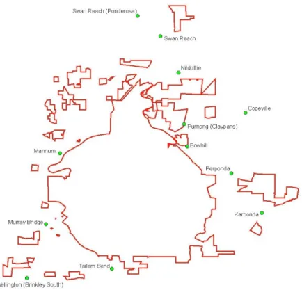
Figure 1. The locations of the Bureau of Meteorology weather stations that measure daily rainfall near the Branched Broomrape Quarantine Area (outlined in red).
Table 2: Branched Broomrape discovery statistics since 2000.
Year Number of “at risk”1 paddocks surveyed (A) Number of infested paddocks found (B) Proportion of infested paddocks (C = B/A) Number of new paddocks found Return rate of known paddocks Starting date of spring surveys 2000 2047 177 0.086 136 39.8% 12 Sep 2001 3145 221 0.070 133 32.0% 18 Sep 2002 3479 52 0.015 11 12.6% 10 Sep 2003 3661 280 0.077 122 40.4% 15 Sep 2004 3727 64 0.017 10 9.87% 20 Sep 2005 3853 97 0.025 13 16.6% 19 Sep * 2006 3982 147 0.037 44 17.5% 11 Sep 2007 4164 105 0.025 17 13.7% 10 Sep 2008 4551 81 0.018 24 8.1% 22 Sep 1
“At Risk” paddocks are those that were surveyed and now fall within the Branched Broomrape Quarantine Area (as of 22/02/09)
The yearly statistics on the branched broomrape season available for analysis include the number of “at risk” paddocks surveyed, the total number of infested paddocks found, the number of new paddocks found with branched broomrape, the return rate for previously known paddocks infested with broomrape and the starting date for surveys (Table 2). The proportion of infested paddocks found was calculated by dividing the number of infested paddocks found by the number of “at risk” paddocks surveyed each year.
In each year, indicator sites were regularly visited prior to the start of surveys to monitor for emerged broomrape plants. Surveys only commenced after emerged plants had been observed. This provides a good date for emergence and thus for 1500 GDD being reached. Therefore, this data can then be used for testing different break of season scenarios.
To determine the date of the break of season (BoS) each year, the GDD curves generated from two rules-of-thumb based on rainfall were compared to predicted date for BoS calculated by assuming that the start of surveys commenced at 1500 GDD. The rules-of-thumb tested were;
10mm of rain falling over two days after April 1st, and 25mm of rain falling over a fortnight ending after April 1st (Figure 2). 2001 and 2004 were the only years where the break of season date was more than two days different using the rules-of-thumb tested. In both of these years
25mm falling over a fortnight was closest to the BoS date generated using the starting date for survey data, therefore, this was used in further analysis of the data and the resulting date for the break of season for each year is displayed in Table 3.
Table 3: Seasonal temperature and rainfall indicators.
Year Date of break of season (based on 25mm in a fortnight) Break of season to 31st Dec (days) Potential period for emergence (days) (From 1500 to 31st Dec) Pre-season rain (mm) (From 1 Jan to break of season) Seasonal rain (mm) (from start to 1500 GDD) Annual rainfall (mm) 2000 13 April 263 150 109.1 146.7 371.7 2001 28 May 218 101 100.7 148.2 343.0 2002 20 May 226 104 69.8 81.4 208.6 2003 20 May 226 104 111.3 185.7 371.4 2004 15 June 200 88 76.7 139.4 325.5 2005 11 June 204 90 85.9 205.8 433.2 2006 28 April 248 127 91.5 88.9 233.1 2007 27 April 249 128 90.9 146.5 335.0 2008 19 May 227 105 49.4 121.8 269.1
Seasonal conditions including the number of days from the break of season to the end of the year, the potential period for emergence to occur (calculated as the number of days from GDD reaching 1500 to the end of the year), annual rainfall, various pre-season rainfall periods (including rainfall between 1st Jan – BoS, 1st Dec – 31st March and 1st Dec - BoS), and growing season rainfall periods (including BoS – 1500 GDD, 1st Apr – 31st Oct, 1st Jan – 31st Oct and 1st Jan – 1500 GDD) were calculated.
Figure 2. Average daily rainfall for the Branched Broomrape Quarantine area (averaged from 12 BoM weather stations) (primary y-axis) and the accumulation of growing degree days to reach 1500 (secondary y-axis) based on the 10mm of rain falling in two days and 25mm of rain falling over a fortnight after April 1st. The estimation of the break of season based on 1500 GDD having accumulated to the date that spring surveys started is shown in blue.
2000 0 10 20 30 40 50 0 1 /0 1 /2 0 0 0 3 1 /0 1 /2 0 0 0 0 1 /0 3 /2 0 0 0 3 1 /0 3 /2 0 0 0 3 0 /0 4 /2 0 0 0 3 0 /0 5 /2 0 0 0 2 9 /0 6 /2 0 0 0 2 9 /0 7 /2 0 0 0 2 8 /0 8 /2 0 0 0 2 7 /0 9 /2 0 0 0 2 7 /1 0 /2 0 0 0 2 6 /1 1 /2 0 0 0 2 6 /1 2 /2 0 0 0 Date R a in fa ll (m m ) 0 200 400 600 800 1000 1200 1400 1600 G D D 2001 0 10 20 30 40 50 0 1 /0 1 /2 0 0 1 3 1 /0 1 /2 0 0 1 0 2 /0 3 /2 0 0 1 0 1 /0 4 /2 0 0 1 0 1 /0 5 /2 0 0 1 3 1 /0 5 /2 0 0 1 3 0 /0 6 /2 0 0 1 3 0 /0 7 /2 0 0 1 2 9 /0 8 /2 0 0 1 2 8 /0 9 /2 0 0 1 2 8 /1 0 /2 0 0 1 2 7 /1 1 /2 0 0 1 2 7 /1 2 /2 0 0 1 Date R a in fa ll (m m ) 0 200 400 600 800 1000 1200 1400 1600 G D D 2002 0 10 20 30 40 50 0 1 /0 1 /2 0 0 2 3 1 /0 1 /2 0 0 2 0 2 /0 3 /2 0 0 2 0 1 /0 4 /2 0 0 2 0 1 /0 5 /2 0 0 2 3 1 /0 5 /2 0 0 2 3 0 /0 6 /2 0 0 2 3 0 /0 7 /2 0 0 2 2 9 /0 8 /2 0 0 2 2 8 /0 9 /2 0 0 2 2 8 /1 0 /2 0 0 2 2 7 /1 1 /2 0 0 2 2 7 /1 2 /2 0 0 2 Date R a in fa ll (m m ) 0 200 400 600 800 1000 1200 1400 1600 G D D 2003 0 10 20 30 40 50 0 1 /0 1 /2 0 0 3 3 1 /0 1 /2 0 0 3 0 2 /0 3 /2 0 0 3 0 1 /0 4 /2 0 0 3 0 1 /0 5 /2 0 0 3 3 1 /0 5 /2 0 0 3 3 0 /0 6 /2 0 0 3 3 0 /0 7 /2 0 0 3 2 9 /0 8 /2 0 0 3 2 8 /0 9 /2 0 0 3 2 8 /1 0 /2 0 0 3 2 7 /1 1 /2 0 0 3 2 7 /1 2 /2 0 0 3 Date R a in fa ll (m m ) 0 200 400 600 800 1000 1200 1400 1600 G D D 2004 0 10 20 30 40 50 0 1 /0 1 /2 0 0 4 2 0 /0 2 /2 0 0 4 1 0 /0 4 /2 0 0 4 3 0 /0 5 /2 0 0 4 1 9 /0 7 /2 0 0 4 0 7 /0 9 /2 0 0 4 2 7 /1 0 /2 0 0 4 1 6 /1 2 /2 0 0 4 Date R a in fa ll (m m ) 0 200 400 600 800 1000 1200 1400 1600 G D D 2005 0 10 20 30 40 50 0 1 /0 1 /2 0 0 5 2 0 /0 2 /2 0 0 5 1 1 /0 4 /2 0 0 5 3 1 /0 5 /2 0 0 5 2 0 /0 7 /2 0 0 5 0 8 /0 9 /2 0 0 5 2 8 /1 0 /2 0 0 5 1 7 /1 2 /2 0 0 5 Date R a in fa ll (m m ) 0 200 400 600 800 1000 1200 1400 1600 G D D 2006 0 10 20 30 40 50 0 1 /0 1 /2 0 0 6 2 0 /0 2 /2 0 0 6 1 1 /0 4 /2 0 0 6 3 1 /0 5 /2 0 0 6 2 0 /0 7 /2 0 0 6 0 8 /0 9 /2 0 0 6 2 8 /1 0 /2 0 0 6 1 7 /1 2 /2 0 0 6 Date R a in fa ll (m m ) 0 200 400 600 800 1000 1200 1400 1600 G D D 2007 0 10 20 30 40 50 0 1 /0 1 /2 0 0 7 2 0 /0 2 /2 0 0 7 1 1 /0 4 /2 0 0 7 3 1 /0 5 /2 0 0 7 2 0 /0 7 /2 0 0 7 0 8 /0 9 /2 0 0 7 2 8 /1 0 /2 0 0 7 1 7 /1 2 /2 0 0 7 Date R a in fa ll (m m ) 0 200 400 600 800 1000 1200 1400 1600 G D D 2008 0 10 20 30 40 50 0 1 /0 1 /2 0 0 8 2 0 /0 2 /2 0 0 8 1 0 /0 4 /2 0 0 8 3 0 /0 5 /2 0 0 8 1 9 /0 7 /2 0 0 8 0 7 /0 9 /2 0 0 8 2 7 /1 0 /2 0 0 8 1 6 /1 2 /2 0 0 8 Date R a in fa ll (m m ) 0 200 400 600 800 1000 1200 1400 1600 G D D 2001 2000 2002 2003 2004 2005 2006 2007 2008
Analysis
Regression analysis was used to investigate for a relationship between the amount of broomrape found and the seasonal conditions experienced. The broomrape discovery statistics were classed as response variables (y) and all climate data were potential explanatory variables (x). All combinations of y and x were plotted in scatter plots against each other in excel and linear trendlines were fitted to estimate the
correlation between the two variables plotted. The x variable “pre-season rain”, calculated as the total volume of rain to fall between 1st Jan and break-of-season, was found to have the strongest correlation of
any of the explanatory variables with the proportion of infested paddocks (r2 = 0.70) (Figure 3a), the return
rate (r2 = 0.75) (Figure 4a) and the number of new paddocks found (r2 = 0.57) (Figure 5). The reciprocal of
“proportion of infested paddocks” provided a slightly better correlation with pre-season rain (r2 = 0.78)
(Figure 3b) and the reciprocal of the return rate with pre-season rain also provided a higher correlation (r2
= 0.89) (Figure 4b). Transformation (e.g. Log10, square-root and reciprocal) of the number of new paddocks did not improve the correlation to pre-season rain. These scatter plots indicate that a linear relationship may not be the best fit. Therefore, using GENSTAT the fit of polynomial curves was investigated.
Results
Proportion of infested paddocks
The cubic regression for the reciprocal of the proportion of infested paddocks (1/y) on pre-season rain (x), 1/y = -517 + 23.39x – 0.2952x2 + 0.001148x3, provided the best fit (r2 = 0.962, P < 0.001). This regression
and the observed proportion of infested paddocks are shown in figure 3 (i.e. Figure 3d has the same data as Figure 3c but it shows y instead of 1/y). Looking at Figure 3c; the quartic regression constantly predicts higher 1/y values than the observed. The quadratic regression doesn’t predict the peak in 1/y values when x is around 70 and also doesn’t predict a plateau when x is >100. Looking at figure 3d: the quartic
regression will always predict a lower proportion of infested paddocks than observed and is least able to predict values when pre-season rain is > 90mm. The quadratic regression has a reasonable fit with the observed data until the pre-season rain is >100mm. The cubic regression shows a downward turn at the last data point (when pre-season rain was >111mm) this may not be reliable and I would be wary of using this equation to predict the extent of broomrape that may be found in a season when pre-season rain doesn’t fall between the range of values used in the analysis.
Return Rate
The quadratic regression for the reciprocal of the return rate (1/y) on pre-season rain (x), 1/y = 16.6 – 0.055x – 0.00068x2, provided the best fit (r2 = 0.868, P < 0.001). This regression and the observed return
rate are shown in figure 4 (i.e. Figure 4d has the same data as Figure 4c but it shows y instead of 1/y). Looking at Figure 4c it is difficult to visually assess which regression most accurately reflects the observed data. Looking at figure 4d, the quartic regression inaccurately predicts the return rate when pre-season rain is > 100mm.
Discussion
This data suggests that the volume of rainfall received during the pre-season period from 1st Jan to the
Break of Season is a more important contributor to the amount of branched broomrape that will emerge in the following season than any of the other seasonal indicators tested.
a) b)
c) d)
Figure 3. Analysis of the proportion of infested paddocks with pre-season rain: a) linear regression of pre-season rain on proportion of infested paddocks, b) linear regression of pre-season rain on the reciprocal of the proportion of infested paddocks, c) polynomial regression of pre-season rain on the reciprocal of the proportion of infested paddocks, showing linear, quadratic, cubic and quartic predictions, d) polynomial regression of pre-season rain on the proportion of infested paddocks, showing linear, quadratic, cubic and quartic predictions.
Observed values excluding 1999
y = 0.0012x - 0.0642 R2 = 0.7031 0 0.02 0.04 0.06 0.08 0.1 25 50 75 100 125 Pre-season rain P ro p _ B B p a d d o c k s
Observed values excluding 1999
y = 0.003x - 0.0701 R2 = 0.7373 0 20 40 60 80 100 25 50 75 100 125 Pre-season rain 1 /P ro p _ B B p a d d o c k s 0 20 40 60 80 100 25 50 75 100 125 Pre-season rain 1 /P ro p _ B B p a d d o c k s
Linear Prediction Quadratic Prediction Cubic Prediction Quartic Prediction Observed 0 0.02 0.04 0.06 0.08 0.1 0.12 0.14 0.16 0.18 0.2 25 50 75 100 125 Pre-season rain P ro p _ B B p a d d o c k s
Linear Prediction Quadratic Prediction Cubic Prediction Quartic Prediction Observed
a) b)
b) d)
Figure 4. Analysis of the return rate of paddocks known to have an infestation with pre-season rain: a) linear regression of pre-season rain on return paddocks, b) linear regression of pre-season rain on the reciprocal of the return paddocks, c) polynomial regression of pre-season rain on the reciprocal of the return paddocks, showing linear, quadratic, cubic and quartic predictions, d) polynomial regression of pre-season rain on the return paddocks, showing linear, quadratic, cubic and quartic predictions.
Observed values excluding 1999
y = 0.0056x - 0.2754 R2 = 0.7505 0 0.1 0.2 0.3 0.4 0.5 0 50 100 150 Pre-season rain R e tu rn R a te
Observed values excluding 1999
y = -0.1656x + 20.867 R2 = 0.8944 0 3 6 9 12 15 0 50 100 150 Pre-season rain 1 /R e tu rn R a te 0 3 6 9 12 15 25 50 75 100 125 Pre-season rain 1 /R e tu rn R a te
Linear Prediction Quadratic Prediction Cubic Prediction Quartic Prediction Observed 0 0.1 0.2 0.3 0.4 0.5 0.6 25 50 75 100 125 Pre-season rain R e tu rn R a te
Linear Prediction Quadratic Prediction Cubic Prediction Quartic Prediction Observed
Figure 5. Linear regression of the number of new paddocks found with an infestation of branched broomrape with pre-season rain
Observed values excluding 1999
y = 2.1499x - 130.92 R2 = 0.5701 0 30 60 90 120 150 0 50 100 150 Pre-season rain N e w P a d d o c k s
4.
Paddock level broomrape infection in relation to
seasonal conditions - Analysis 2
Jane Prider
Branched Broomrape Eradication Program
March 2010
Aim
To investigate the relationship between the number of paddocks found with branched broomrape each year with seasonal conditions such as start of GDD, date of 1500GDD, growing season rainfall etc.
Summary
Growing season rainfall, the timing of the break of season and broomrape emergence showed no correlation with the level of broomrape infection in paddocks. However, there is a non-linear positive relationship between the amount of rainfall occurring between January 1st and the break of season and the
occurrence of broomrape at the paddock scale. Rainfall totalling more than 100 mm in this period is correlated with high levels of infection, whereas rainfall totals up to 100 mm are correlated with low levels of infection. The models predict that in years with wet summers more paddocks will be infected but this is speculative as to date wet years have only occurred during the initial years of the broomrape program when control measures were not as well developed as in more recent years . Pre-season rainfall explains a high proportion of the variance in year to year occurrence of broomrape and it is therefore worthwhile investigating this further to see whether it has causal effects on broomrape occurrence.
Methods
Available data
Daily rainfall data, from 1 Jan 2000 to current, was obtained from the Bureau of Meteorology for twelve weather stations that are located near the branched broomrape quarantine area (Table 1, Fig. 1). The daily rainfall for the district during this period was calculated as the average of these twelve sites.
Table 1: Details for the Bureau of Meteorology weather stations that measure daily rainfall located near the Branched Broomrape Quarantine Area.
Station Number Station Name Latitude Longitude 24517 Mannum Council Depot 34°54'52"S 139°18'04"E 24521 Murray Bridge Comparison 35°07'24"S 139°15'33"E 24535 Swan Reach 34°34'05"S 139°35'50"E 24536 Tailem Bend 35°15'17"S 139°27'15"E 24547 Nildottie 34°40'34"S 139°39'05"E 24572 Wellington (Brinkley South) 35°16'58"S 139°12'11"E 24585 Swan Reach (Ponderosa) 34°30'28"S 139°31'50"E 25002 Purnong (Claypans) 34°49'39"S 139°40'02"E 25003 Copeville 34°47'42"S 139°50'56"E 25006 Karoonda 35°05'24"S 139°53'50"E 25025 Perponda 34°58'24"S 139°48'26"E 25040 Bowhill 34°53'39"S 139°40'36"E
Figure 1. The locations of the Bureau of Meteorology weather stations that measure daily rainfall near the Branched Broomrape Quarantine Area (outlined in red).
In each year, indicator sites were regularly visited prior to the start of surveys to monitor for emerged broomrape plants. Surveys only commenced after emerged plants had been observed. This provides a good date for emergence and thus for 1500 GDD being reached. Therefore, this data was used for testing different break of season scenarios.
To determine the date of the break of season (BoS) each year, the GDD curves generated from two rules-of-thumb based on rainfall were compared to predicted date for BoS calculated by assuming that the start of surveys commenced at 1500 GDD. The rules-of-thumb tested were; 10mm of rain falling over two days after April 1st, and 25mm of rain falling over a fortnight ending after April 1st . 2001 and 2004 were the only years where the break of season date was more than two days different using the rules-of-thumb tested. In both of these years 25mm falling over a fortnight was closest to the BoS date generated using the starting date for survey data, therefore, this was used in further analysis of the data.
Seasonal conditions including the number of days from the break of season to the end of the year, the potential period for emergence to occur (calculated as the number of days from GDD reaching 1500 to the end of the year), annual rainfall, pre-season rainfall periods from December and January to break of season, and growing season rainfall periods (from BoS – 1500 GDD) were calculated (Table 3).
Analysis
Correlations between predictor variables (Table 3) and response variables (Table 2) were calculated using Spearman’s rank correlations. These correlations were tested for a significant departure from the null hypothesis of a random scatter of points (no relationship between predictor and response). Where correlations between variable pairs were significant, linear and second to fourth-order polynomial models were fitted to these data. Each model fit was sequentially tested to determine the minimal model (i.e. the
model with the fewest terms) that adequately described the relationship between the predictor variable and the response variable. This model (or equation) can be used to predict the response variable from a known value of the predictor variable.
Table 2: Branched Broomrape discovery statistics since 2000
Year Number of “at risk”1 paddocks surveyed (A) Number of infested paddocks found (B) Proportion of infested paddocks (C = B/A) Number of new paddocks found Return rate of known paddocks Starting date of spring surveys 2000 2047 177 0.086 136 39.8% 12 Sep 2001 3145 221 0.070 133 32.0% 18 Sep 2002 3479 52 0.015 11 12.6% 10 Sep 2003 3661 280 0.077 122 40.4% 15 Sep 2004 3727 64 0.017 10 9.87% 20 Sep 2005 3853 97 0.025 13 16.6% 19 Sep 2006 3982 147 0.037 44 17.5% 11 Sep 2007 4164 105 0.025 17 13.7% 10 Sep 2008 4551 81 0.018 24 8.1% 22 Sep 2009 4549 47 0.010 6 5.2% 7 Sep
Table 3: Seasonal temperature and rainfall indicators
Year Break of season date (based on 25mm in a fortnight) Break of season to 31st Dec (days) Potential no. days for emergence (from 1500 to 31st Dec) Pre-season rain (mm) (From 1 Jan to break of season) Seasonal rain (mm) (From start to 1500 GDD) Annual rainfall (mm) 2000 13 April 263 150 109.1 146.7 371.7 2001 28 May 218 101 100.7 148.2 343.0 2002 20 May 226 104 69.8 81.4 208.6 2003 20 May 226 104 111.3 185.7 371.4 2004 15 June 200 88 76.7 139.4 325.5 2005 11 June 204 90 85.9 205.8 433.2 2006 28 April 248 127 91.5 88.9 233.1 2007 27 April 249 128 90.9 146.5 335.0 2008 19 May 227 105 49.4 121.8 269.1 2009 27 April 249 135 35.1 100.1 298.1
Results
The only significant seasonal predictor for broomrape infection of paddocks was pre-season rainfall (Table 4). The rainfall that occurs from seed production (end of November) to the break of season was
significantly correlated with the total number of infected paddocks, with this value expressed as a proportion of all “at risk” paddocks, and the return rate. Only the rainfall that fell from January to the break of season was significantly correlated with the number of new paddocks found.
There were also significant correlations between the year and the return rate and the pre-season rainfall from January (Table 4). Scatter plots of these variables show that over time the return rate and pre-season rainfall has declined (Figs 2, 3).
The pre-season rainfall measured from January 1st explained more of the variation in broomrape
occurrence in paddocks than rainfall measured from December 1st so the former data was analysed
further.
Table 4. P-values for Spearman rank correlations between predictor variables and response variables in columns. Shaded cells highlight significant correlations (p < 0.05).
Predictor Number of infected paddocks Number of new infected paddocks Proportion of infected
paddocks Return Rate
Pre-season rain (from Jan) Days from break of season
to emergence 0.894 0.497 0.577 0.96 Potential emergence period 0.96 0.544 0.638 0.987 Year 0.128 0.09 0.09 0.025 0.043 Annual Rain 0.098 0.244 0.074 0.082 Seasonal rainfall 0.054 0.214 0.074 0.074
Pre-season rain (from
Dec) 0.038 0.138 0.019 0.016
Pre-season rain (from Jan) 0 0.003 0 0
Figure 2. There is a significant negative linear decline in pre-season rainfall (from January to break of season) over time.
R² = 0.5109 y = -5.8749x + 11858 0 20 40 60 80 100 120 1998 2000 2002 2004 2006 2008 2010 pr e -s eas o n rai nf al l ( m m ) year
Figure 3. There is a significant negative non-linear (quartic) decline in return rate over time.
The relationship between pre-season rainfall and broomrape occurrence was non-linear. Quadratic polynomial models provided the best minimal fit to all response variables; return rate (Fig. 4), proportion of infected paddocks (Fig. 5), new paddocks and number of paddocks infected (Fig. 6). However, these models provided a poor fit to the lower rainfall values. Cubic polynomial models were also significant and gave a better fit to data points at low rainfall values.
For return rate, the proportion of infected paddocks and new paddocks (Figs 4, 5, 6), there was little change in broomrape occurrence when pre-season rainfall was less than 100 mm. Pre-season rainfall values above 100 mm were correlated with high levels of infected paddocks.
Figure 4. Scatterplot of return rate in relation to rainfall falling between January 1st and the break of season. The quadratic model (solid line) is the minimal model fit but the cubic model (dashed line, equation on chart) provides a better fit for data points at lower rainfall values.
y = 0.0002x4 - 1.5345x3 + 4616.9x2 - 6E+06x + 3E+09 R² = 0.6032 0 0.05 0.1 0.15 0.2 0.25 0.3 0.35 0.4 0.45 1998 2000 2002 2004 2006 2008 2010 ret u rn ra te year y = 2E-06x3 - 0.0004x2 + 0.0213x - 0.3454 R² = 0.9593 0 0.05 0.1 0.15 0.2 0.25 0.3 0.35 0.4 0.45 0 20 40 60 80 100 120 retur n rat e pre-season rainfall (mm)
Figure 5. Scatterplot of proportion of infected paddocks in relation to rainfall falling between January 1st and the break of season. The quadratic model (solid line) is the minimal model fit but the cubic model (dashed line, equation on chart) provides a better fit for data points at lower rainfall values.
Figure 6. Scatterplots of number of new paddocks and total number of infected paddocks found during surveys in relation to rainfall falling between January 1st and the break of season. The quadratic model (solid line) is the minimal model fit but the cubic model (dashed line, equations on chart) provides a better fit for data points at lower rainfall values.
Discussion
Growing season rainfall, the timing of the break of season and emergence showed no correlation with the level of broomrape infection in paddocks. Pre-season rainfall has a significant non-linear correlation with broomrape infection at the paddock level and explains more than 90% of the year to year variance in return rate and the proportion of infected paddocks. The models predict that rainfall above 100 mm during the summer months is critical. Higher return rates, more new infected paddocks and a higher proportion of infected paddocks have all occurred in the growing season following high summer rainfall. However, management of broomrape potentially confounds the results. Two of the wettest years occurred at the beginning of the program (Figs 2, 3), when management of broomrape may not have been as effective as later in the program, as suggested by the low return rates in 2008 and 2009.
y = 3E-07x3 - 5E-05x2 + 0.0022x - 0.0221 R² = 0.927 0 0.01 0.02 0.03 0.04 0.05 0.06 0.07 0.08 0.09 0.1 0 20 40 60 80 100 120 p ro p o rti o n o f in fe cte d p ad d o ck s pre-season rainfall (mm) New paddocks y = 0.0007x3 - 0.1142x2 + 5.595x - 75.286 R² = 0.8384 Infected paddocks y = 0.0006x3 - 0.0753x2 + 3.0016x + 18.225 R² = 0.8494 0 50 100 150 200 250 300 0 50 100 150 n u m b e r o f p ad d o ck s pre-season rainfall (mm) New paddocks Infected paddocks
One of the uses of these models is to be able to predict the severity of broomrape emergence in paddocks from the growing conditions of that year. Cubic models have the best predictive power as they provide a better fit to the data at low rainfall levels. It would be possible to use this model to predict the level of infection in a given year based on the pre-season rainfall. For 2009, a return rate of 8% was predicted and the return rate was 5.2%. The model may provide a useful check on whether management is reducing broomrape occurrence at the paddock level, taking into account seasonal factors.
Although these models show some interesting relationships they have no biological basis. They are useful for formulating questions for further research. The models indicate that seed bank processes have a greater impact on broomrape occurrence than processes that occur during the growing season. Pre-season rainfall has high explanatory power and it is therefore worthwhile investigating this further to see whether it has causal effects on broomrape occurrence.