sparse symmetric indefinite systems
by Olaf Schenk1, and Klaus G¨artner2
Technical Report CS-2004-004
Department of Computer Science, University of Basel Submitted to Electronic Transactions on Numerical Analysis
1Department of Computer Science, University of Basel, Klingelbergstrasse 50,
CH-4056 Basel, Switzerland email: [email protected]
2 Weierstrass Institute for Applied Analysis and Stochastics, Mohrenstr. 39,
D-10117 Berlin, Germany, email: [email protected] I
Technical Report is available at
SYMMETRIC INDEFINITE SYSTEMS
OLAF SCHENK † AND KLAUS G ¨ARTNER ‡
Abstract. This paper illustrates the effectiveness of various new pivoting factorization methods
for solving sparse symmetric indefinite systems. As opposed to many existing pivoting methods, our
Supernode–Bunch–Kaufman pivoting method LDLT−
SBK selects dynamically 1×1 and 2×2 pivots
and is supplemented by static pivoting within the numerical factorization. We demonstrate numerical stability and accuracy of this algorithm and also show that a high performance implementation is feasible. We will also show that symmetric maximum-weighted matching strategies add an additional
level of reliability to LDLT−SBK. Numerical experiments validate these conclusions.
Key words. direct solver, pivoting, sparse matrices, graph algorithms, symmetric indefinite
matrix, interior point optimization
AMS subject classifications.65F05, 65F50, 05C85
1. Introduction. We consider the direct solution of symmetric indefinite linear
systemAx=b, with
A=Pind(PF ill, PMS)LDL
TP
indT(PMS, PF ill) − E,
(1.1)
where D is a diagonal matrix with 1×1 and 2×2 pivot blocks, L is a sparse
lower triangular matrix, Pind is a permutation matrix constructed from structural
(permutation PF ill) and numerical (permutation PMS) information, and E reflects
small static half-machine precision perturbations that might be necessary to maintain
stability. PMS is a reordering that is based on a weighted matching of the matrix
A, and tries to move the largest off-diagonal elements directly alongside the diagonal
in order to form good initial 2×2 or 1×1 diagonal block pivots. PF ill is a fill-in
reducing reordering which honors the block structure ofPMS.
Sparse symmetric indefinite linear systems arise in numerous areas ranging e.g. from incompressible flow computations, to linear and nonlinear optimization, electro-magnetic scattering, finite element analysis and in shift-invert eigensolvers, even when
the original matrix A is sought to be symmetric positive definite. In general, some
kind of pivoting techniques must be applied in order to solve these systems accurately and the challange is to achieve numerical stability and sparsity of the factors.
1.1. Previous Work. Extensive investigation on pivoting techniques for
sym-metric indefinite direct solvers have been done by numerous researchers. There are three well known algorithms for solving dense symmetric indefinite linear systems: the Bunch-Kaufman algorithm [7], the Bunch-Parlett algorithm [8], and Aasen’s method [1]. The most recent algorithmic paper on pivot search and pivot-admissibility is [3] and the authors proposed a bounded Bunch-Kaufman pivot selection for bounding the numerical values of the factor. In this paper, we will always apply the
Bunch-Kaufman pivoting selection since it is also part of theLapackcodeDsytrfVersion
∗This work was supported by the Swiss Commission of Technology and Innovation under contract
number 7036.1 ENS-ES and the HP Integrity for Research Program at WIAS.
†Department of Computer Science Department, University Basel, Klingelbergstrasse 50, CH-4056
Basel, Switzerland, ([email protected]).
‡Weierstrass Institute for Applied Analysis and Stochastics, Mohrenstr. 39, D-10117 Berlin,
Germany, ([email protected]).
3.0 that we use within the factorization. However, the bounded Bunch-Kaufman algorithm may be another potential pivoting strategy that we might investigate in future research. For further details on symmetric pivoting techniques, and stability and accuracy issues see [14, 21] and the references therein.
In [24, 25] the new static pivoting approach in SuperLU is presented for the
factorization of sparse nonsymmetric systems. This method needs an additional pre-processing step based on weighted matchings [11] which reduces the need for partial pivoting thereby speeding up the solution process. More recently, in [13] scalings strategies based on symmetric weighted matchings have been investigated and rea-sonable improvements are reported for symmetric indefinite systems. Another recent contribution is [26], which discusses high-performance in-core and out-of-core sparse symmetric indefinite algorithms and implementations.
1.2. Contributions of the paper. We conduct an extensive study on the use
of Bunch and Kaufman pivoting using 1×1 and 2×2 pivots, followed by static
pivoting techniques for the factorization of sparse symmetric indefinite systems. To the best of our knowledge, our algorithm techniques is the first pivoting method, which uses both dynamic and static pivoting for symmetric indefinite systems, to be proposed. Furthermore, we also consider symmetric permutations based on numerical indistinguishable vertices and local modifications in the context of symmetric weighted matchings. The use of weighted matchings in combination with our pivoting method is new — similar techniques in combination with other pivoting methods have recently been proposed in [10] and explored in [13, 15, 28].
While we do not claim that this approach to factor symmetric indefinite systems will always work, we do hope that the results in this paper will contribute to further acceleration for direct solvers for sparse indefinite systems. We also hope that the combination of our pivoting methods and symmetric weighted matchings will find widespread use in the area of hard to solve symmetric indefinite linear systems. Our implementation of the new method is reliable and performs well. On a 2.4 GHz Intel 32-bit processor, it factors an indefinite symmetric Karush-Kuhn-Tucker (KKT) optimization example with about 2 millions rows and columns in less than one minute,
producing a factor with about 1.4×10⁸nonzeros.
The paper is organized as follows. Section 2 provides some background on sym-metric indefinite factorizations and presents our formulation of the factorization using
1×1 and 2×2 pivots. We follow this with a discussion of additional preprocessing
methods based on symmetric weighted matchings in Section 3 and 4. Finally, Section 5 presents our numerical results for sparse matrices from a wide range applications. Section 6 presents our conclusions.
2. TheLDLT−SBKalgorithm. Virtually all modern sparse factorization codes
rely heavily on a supernodal decomposition of the factor L to efficiently utilize the
memory hierarchies in the hardware as shown in Figure 2.1. The factor is decomposed
into dense diagonal blocks of size ns and into the corresponding subdiagonal blocks
such that the rows in the subdiagonals are either completely zero or dense. There are two main approaches in building these supernodes. In the first approach, consecutive
rows and columns with the identical structure in the factor L are treated as one
fundamental supernode. These supernodes are so crucial to high performance in sparse matrix factorization that the criterion for the inclusion of rows and columns in the same supernode can be relaxed [4] to increase the size of the supernodes. This is the second approach and it is called supernode amalgamation. In this approach consecutive rows and columns with nearly the same but not identical structures are
A= LD=
Fig. 2.1.Illustration of the fundamental supernodal decomposition of the factor for a
symmet-ric indefinite matrixA. The filled circles correspond to elements that are nonzero in the coefficient
matrixA, non-filled circles indicate elements that are zero and explicitly stored, the dotted circles
indicate zeros in the factor that are stored in the supernode structure but not accessed during nu-merical factorization, and triangles represent fill elements. The filled boxes indicate the diagonal supernode structure where Bunch-Kaufman pivoting is performed and the dotted boxes indicate the remaining part of the supernodes.
included in the same supernode, and artificial nonzero entries with a numerical value of zreo are added to maintain identical row and column structures for all members of a supernode. The rationale is that the slight increase in the number of nonzeros and floating-point operations involved in the factorization can be compensated by a higher factorization speed. In this paper, we will always use a fundamental supernodal decomposition with the extension that we add explicitly zeros in the upper triangular
part ofLin order to form a rectangular supernode representation that can be factored
using optimizedLapackroutines.
Algorithm 2.1. LDLT supernode Bunch-Kaufman pivot selection with
half-maschine precision perturbation.
1. γ1= maxk=2,...n|ak1|
2. γr≥γ1is the magnitude of the largest off-diagonal in the r−row.
3. if max(|a11|, γ1)≤:
4. use static pivot perturbation: a11=sign(a11)×
5. use perturbed a11as a1×1pivot.
6. else if |a11| ≥αγ1: 7. usea11as a1×1pivot. 8. else if |a11| ×γr≥αγ12: 9. use|a11|as a1×1pivot. 10. else if |arr| ≥αγr: 11. use|arr|as a1×1pivot. 12. else 13. use a11 ar1 ar1 arr as a2×2pivot
We will use a Level-3Blasleft-looking factorization as described in [29, 30]. An
interchange among the rows and columns of a supernode of diagonal sizens, referred
to as dynamic supernode Bunch-Kaufmann pivoting, has no effect on the overall
fill-in and this is the mechanism for finding a suitable pivot in our LDLT −SBK
method. However, there is no guarantee that the numerical factorization algorithm would always succeed in finding a suitable pivot within the supernode block. When the algorithm reaches a point where it cannot factor the supernode based on the previously
described 1×1 and 2×2 pivoting, it uses a pivot perturbation strategy similar to [25].
The magnitude of the potential pivot is tested against a constant threshold of, where
is a half-maschine precision perturbation. Therefore, any tiny pivots encountered
during elimination are set to sign(aii)·— this trades off some numerical stability for
the ability to keep pivots from getting too small. The result of this pivoting approach is that the factorization is, in general, not accurate and iterative refinement may be needed. Furthermore, when there are a small number of pivot failures, they corrupt
only a low dimensional subspace and each perturbation is a rank−1 update of A,
so iterative refinement can compensate for such corruption with only a few extra
iterations. Algorithm 2.1 describes the 1×1 and 2×2 Bunch-Kaufman pivoting
strategy with static half-maschine precision perturbation. To factor the individual
supernodes we incorporated this pivoting strategy into theLapackcode Dsytrf, a
right-looking indefinite factorization code.
3. Weighted Matchings. Numerical stability in the factorization is typically
maintained through pivoting, which can have a critical impact on the factorization speed. Unfortunately, row and column interchanges due to pivoting can unpredictably affect the non-zero structure of the factor, thus making it impossible to statically allo-cate data-structures. The motivation of the weighted matching approach is to restrict the pivoting during the factorization phase by obtaining a good initial pivoting or-der through a weighted matching in an additional preprocessing step. The idea to
use weighted matchingsPMas a static approximation of the pivoting order for
non-symmetric dense linear systems was firstly introduced in [27] and [11] is a significant
extension to sparse nonsymmetric systems. Permuting the rowsA ← PMA or the
columnsA ← APMof the sparse system to ensure a zero-free diagonal or to maximize
the product of the absolute values of the diagonal entries are techniques that are now often regularly used in direct and also iterative linear solvers [6, 24, 29, 31].
Until recently, only nonsymmetric permutations were considered. In [10] ideas
are presented on how to modify nonsymmetric matchingsPMfor the solution of
sym-metric systems while maintaining the symmetry of the permuted systemPMSAPMS
using a desired symmetric matchingMS. This work was a preliminary presentation
of the idea and [13, 15, 28] implemented and extended these methods in order to find good scalings and pivoting orderings for symmetric indefinite systems.
3.1. Matching Algorithms. An important reason for the success of weighted
matchings in current state-of-the art sparse solvers is the practical efficiency of these algorithms. They rely on associate graph representations of the matrices. In our case,
the algorithms work on abipartite graphGA= (Vr, Vc, E), whereVrandVcare vertex
sets of cardinalityN, representing the rows and columns of the matrix, respectively,
and E ={(i, j)|aij 6= 0}is the set of edges connecting the vertices in Vr and Vc.
Now, we are looking for a subsetM ⊆ E with the following properties: (a) for all
verticesv ∈ {Vr, Vc}, exactly one edge e∈ M is incident tov, and (b) the matched
edgese∈ Mmaximize a weight functionw(·), with
w(M) = X
(i,j)∈M
C(A)ij (3.1)
whereC(A) is a weight coefficient matrix that depends on the matrixA.
Such a subset M is called a perfect weighted matching of GA. The problem of
finding it is called abipartite weighted matching problem and the first condition can
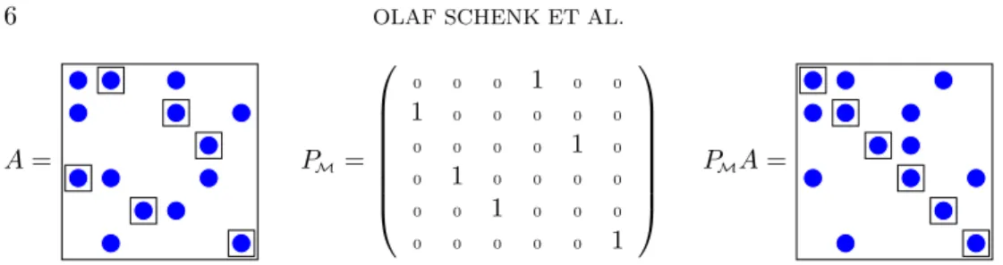
A= PM= 0 0 0 1 0 0 1 0 0 0 0 0 0 0 0 0 1 0 0 1 0 0 0 0 0 0 1 0 0 0 0 0 0 0 0 1 PMA=
Fig. 3.1. Illustration of the row permutation. The matched entries are marked with squares.
The permutation matrixPM is constructed as in (3.4).
matching algorithms are based on the principle of shortest augmenting paths. The
original algorithm, which is also calledHungarian method, is based on Kuhn’s idea [23].
A method based on augmented paths to compute matchings for sparse nonsymmetric
matrices has been used in [11] and an upper bound ofO(n(τ +kn) logn) is given in
[18]. However, experimental results confirm that the complexity is often significantly lower than this upper bound. Thus, the determination of the matching is expected to be in most cases only a minor part of the overall work, and negligible compared to the factorization, which we have also observed in our numerical experiments in Section 5.
3.2. Weight Criteria. An important consideration for the matching is the
choice of the weighting function C(A). As the matching algorithms typically
max-imize (3.1), the criterion has to be formulated in terms of the weight coefficientscij.
If we want to maximize thesum of the matched entries inA, the coefficient matrixC
can simply be defined as
cij =|aij|
(3.2)
The maximization of theproduct of the matched entries inAcan be acquired by using
the logarithm: cij = log|aij| ifaij6= 0, −∞ otherwise. (3.3)
Other variants are discussed in [11, 18]. All algorithms have in common that the coefficients are modified, either for a better performance of the matching, or to enforce the above conditions. See [18] for a survey of such techniques. Experimental results
suggest that themaximum product approach is generally the most beneficial method
[6, 12, 31].
3.3. Nonsymmetric Permutations. As soon as we have computed a weighted
matching, we can construct a corresponding permutation matrixPMwhich permutes
the rows or columns of the matrix such that the matched entries ofAare moved onto
the diagonal: (PM)ij = 1 if (j, i)∈ M 0 otherwise (3.4)
This is illustrated in Figure 3.1. In the permuted systemsPMA the matched, large
by modulus entries occur on the diagonal. While this approach may also be used for symmetric matrices, it has the undesirable drawback that the symmetry of the original system is destroyed.
3.4. Symmetric 1×1 and 2×2 block weighted matchings. In the case
of symmetric indefinite matrices, we are looking for a permutationPMSAPMS that
maintains symmetry. In addition, we impose the property that most of the matched
elements are permuted onto diagonal blocks of preferable 1×1 and 2×2 block size
to serve as initial pivot blocks for the LDLT −SBK factorization method. It can
be shown that the problem of finding symmetric weighted matchings in a symmetric matrix is equivalent to finding a matching in an undirected graph [13]. While these findings may be helpful in devising a special matching algorithm for this problem, to the best of our knowledge no such method exists as of today. We therefore deploy the
well-established general weighted matchingsPMand construct the desired symmetric
matchingPMS in an additional step, which has a linear complexity.
An observation on how to buildPMS from the information given by a weighted
matching PM was presented in [10]. It is noticed that the cycle structure of the
permutationPM can be exploited to derive such a permutation PMS. Cycle
repre-sentations are natural in the context of permutations. For example, the permutation
PM from Figure 3.1 can be written in cycle representation as
PM= (124)(35)(6).
(3.5)
A 1-cycle in this cycle representation corresponds to a diagonal element, that is — in terms of the weight criterion of the matching — the optimal element in its row and column. A cycle of length two can be seen as the representation of two large
symmetric off-diagonal elements aij and aji paired with two possibly small or even
zero diagonal elements aii and ajj. Any permutation ˜P mapping the nodes in the
cycleci of lengthl(ci) on (k, k+ 1, . . . , k+l(ci)−1,k=Pi −1 1 l(cj)) will result in a symmetric matrix ˜ A= ˜PAP˜T
having diagonal blocks of cycle lengthesl(cj) size containing all the matched elements
ofA. The fill-in corresonding to permutations of that class may be prohibitive large.
The cycles corresponding toPM are broken up into disjoint 2×2 and 1×1 cycles
c1, . . . , ckand the total length of all cycles sum up to the dimension ofA. These cycles
are used to define a symmetric permutationσ= (c1, . . . , ck), which is the permutation
PMS. One has to distinguish between cycles of even and odd length. It is possible
to break up even cycles into cycles of length two. For each even cycle, there are two possibilities to break it up. We use a structural metric [10] to decide which one to take. The same metric is also used for cycles of odd length, but the situation is
slightly different. Cycles of length 2k+ 1 must be broken up into kcycles of length
two and one cycle of length one. There are 2k+1 different possibilities to do this. The
resulting 2×2 blocks will contain the matched elements ofPM. However, there is no
guarantee that the remaining diagonal element corresponding to the cycle of length one will be nonzero. Our current implementation will randomly select one element
as a 1×1 cycle from an odd cycle of length 2k+ 1. If this diagonal element aii is
still zero during the numerical factorization, it will be perturbed using the strategies described in Section 2.
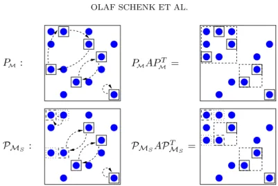
A selection of PMS from a weighted matching PM is illustrated in Figure 3.2.
The weighted matching consists of PM = (124)(35)(6) and the odd cycle of length
three is split into two cycles (1)(24) — resulting in PMS = (1)(24)(35)(6). If PMS
PM : PMAPMT =
PMS : PMSAP
T MS =
Fig. 3.2. Illustration of a symmeric permutation with PM = (124)(35)(6) and PMS =
(1)(24)(35)(6). The split matchingPMS has two additional elements (indicated by dashed boxes),
while one element of the original matching fell out (dotted box). The two 2-cycles are permuted into
2×2diagonal blocks to serve as initial2×2pivots.
the weighted matching will be permuted close to the diagonal and these elements will
form good initial 1×1 and 2×2 pivots for the subsequent LDLT−SBK factorization.
Good fill-in reducing orderingsPF ill are equally important for symmetric
indefi-nite systems and the following section gives a detailed account on how to combine these
reorderings with the matchingPMS. The resulting permutationPind(PF ill,PMS) is
derived usingPMS based on the numerical criterion and alsoPF illbased on structural
criterion will provide good initial pivots for the LDLT−SBK factorization as well as
a good fill-in reduction permutation.
4. Symmetric orderings based on numerical criterionsPMS and
struc-tural criterionsPF ill. In order to construct the factorization efficiently, care has to
be taken that not too much fill-in is introduced during the elimination process. We now examine two alternatives for the combination of reorderings based on weighted
matchings and the fill-in reorderings based on e.g. the Metis nested dissection
re-ordering [22].
4.1. Fill-in reductions PF ill based on numerical indistinguishable
ver-tices. In order to combine thePMS reordering with a fill-in reducing reordering, we
compress the graph of the reordered systemPMSAP
T
MS and apply the fill-in
reduc-ing reorderreduc-ing to the compressed graph. In the compression step, the union of the
structure of the two rows and columns corresponding to a 2×2 diagonal block are
built, and used as the structure of a single, compressed row and column represent-ing the original ones. Graph compression is an important technique that is critical for achieving best performance in modern codes [2]. To explain the rationale behind
graph compression, we must definenumerical indistinguishable vertices.
Definition 4.1. Given an undirected graphGA= (V, E), two verticesv, w∈V are numerically indistinguishable if and only if there exists an edge(v, w)∈E, andv
andw form a 2-cycle inPMS.
Numerical graph compression is the practice of finding sets of numerical
in-distinguishable vertices (v, w) ∈ V and replacing them with a single supervertex
u={u, v} ∈Vc in the compressed graphGc = (Vc, Ec). An edgeec= (s, u)∈Ec
of the following edges exits inE : (s1, u1),(s1, u2),(s2, u1) or (s2, u2). The fill-in
re-ducing ordering can be performed on the numerically compressed graphGc= (Vc, Ec)
with the understanding that members of a supervertex are numbered sequentially. All
verticesuassociated with 1−cycles will form a supervertexu={u, u}of size one in
Gc.
Algorithm4.2. Pseudo-code for the compressed graph approach based on nu-merical indistinguishable vertices.
1. M =build mps matching (A) 2. match cycles =get cycle repr (M)
3. split cycles =split cycle repr (match cycles)
4. (PMS, cyc index) =build numerical perm (split cycles)
5. Gc =compress matrix(PMSAP
T
MS,cyc index)
6. Pc =build metis reordering (Gc)
7. PF ill =expand reordering (Pc,cyc index)
8. Aˆ =PF illPMS A P
T MSP
T F ill
Algorithm 4.2 illustrates all components of the ordering based on numerical
in-distinguishable vertices. First, the weighted matchingPMand the corresponding 1×1
and 2×2 cycle representation is computed. In the next three steps, we determine
PMS using Algorithm 4.3 according to the information incyc index(s) that indicates
whether a vertex is a member of a 1−cycle or a 2−cycle. The numerically compressed
graph based on PMSAP
T
MS is determined and reordered using Metis. Finally, we
expand the compressed permutationPc toPF ill and apply the ordering toPMS with
Pind=PF illPMS.
Algorithm4.3. Construction of a reordering based on cycle representation.
1. function: (P,cyc index) =build numerical perm(split cycles)
2. i←1
3. P ←0∈Rn×n
4. cyc index←0∈Rn
5. forcycleγin split cycles: 6. ifγ= (s)is a 1-cycle: 7. cyc index(s)←1 8. Pi,s←1; i←i+ 1 9. ifγ= (s, t)is a 2-cycle: 11. Pi,s←1; i←i+ 1 12. Pi,t←1; i←i+ 1
15. return(P,cyc index)
4.2. Local modifications of the global fill-in reductionPF ill using PMS.
A second alternative for the combination of reorderings based on weighted matchings and fill-in reducing orderings is discussed in this section. The method is based
pri-marily on a global fill-in reduction of the adjacency graph GA ofA combined with
local modifications according to the weighted matching PMS. The Algorithms 4.4
and 4.5 illustrate the main components of the method.
Algorithm4.4. Pseudo-code local modifications of the global fill-in reduction method usingPMS.
1. M =build mps matching (A) 2. match cycles =get cycle repr (M)
3. split cycles =split cycle repr(match cycles)
4. (PMS, cyc index) =build numerical perm (split cycles)
7. PF ill =local mod reordering (PA, cyc index) 8. Aˆ =PF illPMS A P T MSP T F ill
The first four steps are identical to Algorithm 4.2 and we immediately see that
theMetisreorderingPAis applied to GA instead to the supervertex graphGc. The
next step is shown in detail in Algorithm 4.5. The method traverses the ordering
PAand immediately accepts a vertex that corresponds to a 1−cycle. If a vertexsis
traversed that corresponds to a 2−cycleγ= (s, t), this vertex is also accepted if the
counter vertext is already marked. In this case, we will accept the vertex with the
largest diagonal element|ass|or|att| first. If the counter vertextis not yet marked,
we will not accept node s, pass it for later processing, and mark both nodes t and
s. This strategy can be viewed as a delayed pivoting algorithm during the analysis
phase and it has the beneficial impact that 2×2 initial pivoting diagonal blocks are
preserved while at the same time maintaining a good fill-in reducing ordering.
Algorithm4.5. Local modification based on cycle representation.
1. function: Q=local mod reordering(PA, cyc index )
2. i←1;Q←0∈Rn×n 3. fork= 1, ..., n 4. vertexs=PA(k); 5. ifγ= (s)is a 1-cycle: 6. Qi,s←1; i←i+ 1 7. else 8. γ= (s, t)is a 2-cycle 9. ifvertext already marked
10. Qi,s←1; i←i+ 1 or Qi,t←1 i←i+ 1
11. Qi,t←1; i←i+ 1 Qi,s←1 i←i+ 1
12. else
13. delay vertexs; mark vertextands;
15. returnQ
5. Numerical Experiments. We now present the results of the numerical
ex-periments that demonstrate the robustness and the effectiveness of our pivoting ap-proach.
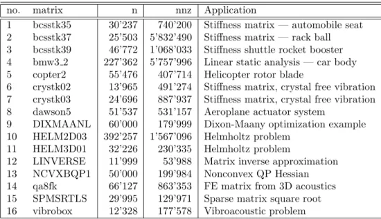
5.1. Sparse Symmetric Indefinite Matrices. The test problems employed
in this research can be classified as being either of augmented symmetric indefinite type A= A11 B BT 0
or of general symmetric indefinite type. The matrices A11 and B in the augmented
systemAare large and sparse, and no assumption is made for the upper left blockA11.
Most of the test problems are taken from extensive surveys [16, 17, 32] of direct solvers
for 61 indefinite systems1. This set is rather challenging and several of the matrices
could not be solved by some of the sparse direct solvers under the constraints imposed in the reports [16, 17, 32]. The matrices comprise a variety of application areas and Table 5.1 and 5.2 give a rough classification of the matrices including the number of unknowns, the number of zero diagonal elements, the total number of nonzeros in the matrix, and the application area. In addition to these matrices, Table 5.2 also
1
no. matrix n nnz Application
1 bcsstk35 30’237 740’200 Stiffness matrix — automobile seat
2 bcsstk37 25’503 5’832’490 Stiffness matrix — rack ball
3 bcsstk39 46’772 1’068’033 Stiffness shuttle rocket booster
4 bmw3 2 227’362 5’757’996 Linear static analysis — car body
5 copter2 55’476 407’714 Helicopter rotor blade
6 crystk02 13’965 491’274 Stiffness matrix, crystal free vibration
7 crystk03 24’696 887’937 Stiffness matrix, crystal free vibration
8 dawson5 51’537 531’157 Aeroplane actuator system
9 DIXMAANL 60’000 179’999 Dixon-Maany optimization example
10 HELM2D03 392’257 1’567’096 Helmholtz problem
11 HELM3D01 32’226 230’335 Helmholtz problem
12 LINVERSE 11’999 53’988 Matrix inverse approximation
13 NCVXBQP1 50’000 199’984 Nonconvex QP Hessian
14 qa8fk 66’127 863’353 FE matrix from 3D acoustics
15 SPMSRTLS 29’995 129’971 Sparse matrix square root
16 vibrobox 12’328 177’578 Vibroacoustic problem
Fig. 5.1.General symmetric indefinite test matrices. ndenotes the total number of unknowns,
andnnzthe nonzeros in the matrix.
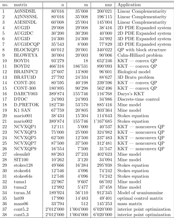
shows two augmented symmetric indefinite matriceslnt09andmass06from [20] and
two large augmented sparse indefinite systemscont5 2andcont5 3from the interior
point optimization package Ipopt [33]. The matrices have been especially included
in order to demonstrate the robustness benefit due to symmetric weighted matchings as an additional preprocessing strategy for symmetric indefinite sparse factorization methods.
5.2. Test Environment and Codes. All numerical tests were run on a double
processor Pentium III 1.3 GHz system with 2 GB of memory, but only one processor was used for the testing. The system runs a recent Linux distribution. In order to
provide realistic measurements, the timings were determined using thegettimeofday
standard C library function, which provides a high accuracy wall clock time. To compensate for the variations, we provide the best result out of three runs for each measurement.
All algorithms were implemented in Fortran 77 and C and were integrated into thePardisosolver package2, a suite of publicly available parallel sparse linear solvers.
The code was compiled byg77and gccwith the -O3 optimization option and linked
with the Automatically Tuned Linear Algebra SoftwareAtlaslibrary3 for the basic
linear algebra subprograms optimized for Intel architectures. The weighted matching
codemps, which is part of thePardisopackage, was provided by Stefan R¨ollin from
ETH Zurich, and it is based on [18]. In general, the performance and the results of
thempscode are comparable to themc64code from the HSL library [19].
In all numerical experiments in Section 5.5, right-hand side vectorsb=A ·1are
computed so that the exact solutionxis equal tox=1. In Section 5.6 we used the
original right-hand side that was generated by the interior point optimization package. For all our tests, scaling was found to make an insignificant difference and hence we
2http://www.computational.unibas.ch/cs/scicomp/software/pardiso 3https://sourceforge.net/projects/math-atlas
no. matrix n m nnz Application
1 A0NSDSIL 80’016 35’008 200’021 Linear Complementarity
2 A2NNSNSL 80’016 35’008 196’115 Linear Complementarity
3 A5ESINDL 60’008 25’004 145’004 Linear Complementarity
4 AUG2D 29’008 29’008 38’416 2D PDE Expanded system
5 AUG2DC 30’200 30’200 40’000 2D PDE Expanded system
6 AUG3D 24’300 24’300 34’992 3D PDE Expanded system
7 AUG3DCQP 35’543 8’000 77’829 3D PDE Expanded system
8 BLOCKQP1 60’012 20’001 340’022 QP with block structure
9 BLOWEYA 30’004 20’003 90’006 Cahn-Hilliard problem
10 BOYD1 93’279 18 652’246 KKT — convex QP
11 BOYD2 466’316 186’531 890’093 KKT — convex QP
12 BRAINPC2 27’607 13’800 96’601 Biological model
13 BRATU3D 27’792 24’334 88’627 3D Bratu problem
14 CONT-201 80’595 40’198 239’596 KKT — convex QP
15 CONT-300 180’895 90’298 562’496 KKT — convex QP
16 DARCY003 389’874 155’746 116’768 Darys’s KKT
17 DTOC 24’993 24’993 34’986 Discrete-time control
18 D PRETOK 182’730 53’570 885’416 Mine model
19 K1 SAN 67’759 20’805 303’364 Mine model
20 mario001 38’434 15’304 114’643 Stokes equation
21 mario002 389’874 155’746 1’167’685 Stokes equation
22 NCVXQP1 12’111 5’000 40’537 KKT — nonconvex QP
23 NCVXQP3 75’000 25’000 324’982 KKT — nonconvex QP
24 NCVXQP5 62’500 12’500 237’483 KKT — nonconvex QP
25 NCVXQP7 87’500 37’500 312’481 KKT — nonconvex QP
26 NCVXQP9 16’554 7’500 31’547 KKT — nonconvex QP
27 olesnik0 88’263 27’233 402’623 Mine model
28 SIT100 10’262 3’120 34’094 Mine model
29 stokes128 49’666 16’384 295’938 Stokes equation
30 stokes64 12’546 4’096 74’242 Stokes equation
31 stokes64s 12’546 4’096 74’242 Stokes equation
32 tuma1 22’967 9’607 66’592 Mine model
33 tuma2 12’992 5’477 37’458 Mine model
34 turan M 189’924 56’110 912’345 Model of uraniummine
35 lnt09 17’990 14’483 49’401 optimal control matrix
36 mass06 33’794 512 145’253 mass matrix
37 cont5 2 2’012’000 1’004’000 6’020’000 interior point optimization
38 cont5 3 2’012’000 1’004’000 6’020’000 interior point optimization
Fig. 5.2. Augmented symmetric indefinite test matrices. n denotes the total number of
un-knowns,mthe number of zero diagonals, andnnz the nonzeros in the matrix.
do not report on the effects on scalings here.
We used two steps of iterative refinement in cases where perturbations have been performed during the numerical factorization and a factorization is considered to be successful if the residual
kb− Axk < (kAk kxk+kbk)
is smaller than= 10−4. This corresponds to the same accuracy as used by Gould
and Scott in [17]. We also consider a factorization as not successful, if the residual significantly grows during one iterative refinement process.
5.3. Performance Profiles. In order to evaluate the quality of the different
pivoting methods for symmetric indefinite linear systems we used performance profiles as a tool for benchmarking and for comparing the algorithms. Theses profiles were firstly proposed in [9] for benchmarking optimization software and recently used in [16, 17, 32] to evaluate various sparse direct linear solvers.
The profiles are generated by running the set of pivoting methodsMon our set
of sparse matrices S and recording information of interest e.g. time for numerical
factorization, memory consumption and residual accuracy. Let us assume that a
pivoting methodm∈ M reports a statistictms ≥0 for the sparse indefinite matrix
s ∈ S and that a smaller statistic tms indicates a better solution strategy. We can
further define ˜ts= min{tms, m∈ M }, which represents the best statistic for a given
sparse matrixm. Then forα≥0 and eachm∈ Mands∈ S we define
k(tms,˜ts, α) =
1 iftms≤α˜ts
0 otherwise.
(5.2)
The performance profilepm(α) of the pivoting methodmis then defined by
pm(α) =
P
s∈Sk(tms,˜ts, α)
|S|
(5.3)
Thus, in these profiles, the values ofpm(α) indicate the fraction of all examples, which
can be solved withinαtimes, the best strategy e.g. pm(1) gives the fraction of which
pivoting methodmis the most effective method and limα→∞indicates the faction for
which the algorithm succeeded.
5.4. Factorization Pivoting Algorithms. Apart from our new approach based
on dynamic supernode Bunch and Kaufman pivoting followed by static pivoting, we provide comparisons with several other symmetric factorization pivoting methods as well as with symmetric matchings as an additional preprocessing method. In partic-ular, we will consider the following options:
CHOLESKY LLT factorization for symmetric positive definite
systems. The diagonal elements of all test matri-ces are changed in such a way that the resulting symmetric system is positive definite.
LDLT LDLT factorization with diagonal pivoting.
LDLT−SBK LDLT factorization with supernode Bunch and
Kaufman using 1×1 and 2×2 pivoting, followed
by static pivoting if the actual pivot is less than
= 10−8 in absolute value.
LDLT−CM−SBK LDLT factorization with symmetric matchings
based on compressed numerical indistinguishable
vertices, supernode Bunch and Kaufman using 1×1
and 2×2 pivoting, followed by static pivoting if the
actual pivot is less than= 10−8in absolute value.
LDLT−M−SBK LDLT factorization with symmetric matchings
based on local modification of the original adja-cency graph, supernode Bunch and Kaufman using
1×1 and 2×2 pivoting, followed by static pivoting
if the actual pivot is less than= 10−8in absolute
value.
We always usedMetis[22] to symmetrically reorder the rows and columns of all
matrices prior to factoring them. This is either performed on the original adjacency
graph for the methods CHOLESKY, LDLT, LDLT−SBK and LDLT−M−SBK or on
the compress 1×1 and 2×2 subgraph for the method LDLT−CM−SBK. We have
also included the CHOLESKY factorization in the numerical experiments in order to show the absolute performance of the indefinite symmetric pivoting methods. This performance profile represents in most of the cases an upper bound and it is useful to assess the quality of the algorithms for indefinite systems.
1 1.5 2 2.5 3 3.5 4 4.5 5 0 0.1 0.2 0.3 0.4 0.5 0.6 0.7 0.8 0.9 1
Performance Profile: AFS.CPU − 16 general indefinite symmetric problems
α
fraction of problems for which solver within
α of best CHOLESKY LDLT (3 failed) LDLT − SBK (0 failed) LDLT − CM − SBK (0 failed) LDLT − M − SBK (0 failed) 1 1.5 2 2.5 3 3.5 4 4.5 5 0 0.1 0.2 0.3 0.4 0.5 0.6 0.7 0.8 0.9 1 α
fraction of problems for which solver within
α
of best
Performance Profile: AFS.CPU − 38 augmented indefinite symmetric problems
CHOLESKY LDLT (32 failed)
LDLT − SBK (4 failed)
LDLT − CM − SBK (1 failed)
LDLT − M − SBK (1 failed)
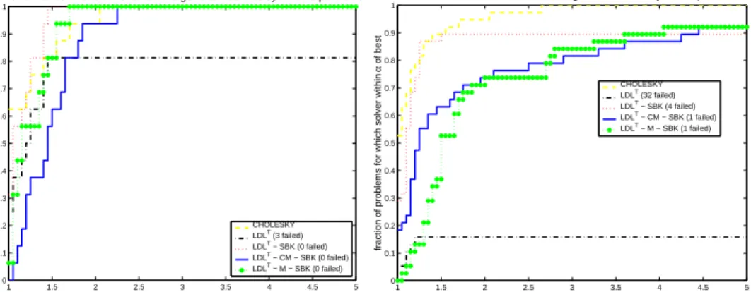
Fig. 5.3. Performance profile CPU time for the complete solution (analysis, factor, solve) for
both sets of symmetric indefinite matrices.
5.5. Numerical results for augmented and general symmetric indefinite
systems. We present the performance profiles for the CPU time for the complete
solution process including analysis, factorization, solve and potentially iterative re-finement in Figure 5.3. In Figure 5.3 and all other Figures 5.4 to 5.6 the left graphic
1 1.5 2 2.5 3 3.5 4 4.5 5 0 0.1 0.2 0.3 0.4 0.5 0.6 0.7 0.8 0.9 1
Performance Profile: Analysis.CPU − 16 general indefinite symmetric problems
α
fraction of problems for which solver within
α of best CHOLESKY LDLT (3 failed) LDLT − SBK (0 failed) LDLT − CM − SBK (0 failed) LDLT − M − SBK (0 failed) 1 1.5 2 2.5 3 3.5 4 4.5 5 0 0.1 0.2 0.3 0.4 0.5 0.6 0.7 0.8 0.9 1 α
fraction of problems for which solver within
α
of best
Performance Profile: Analysis.CPU − 38 augmented indefinite symmetric problems
CHOLESKY LDLT (32 failed)
LDLT − SBK (4 failed)
LDLT − CM − SBK (1 failed)
LDLT − M − SBK (1 failed)
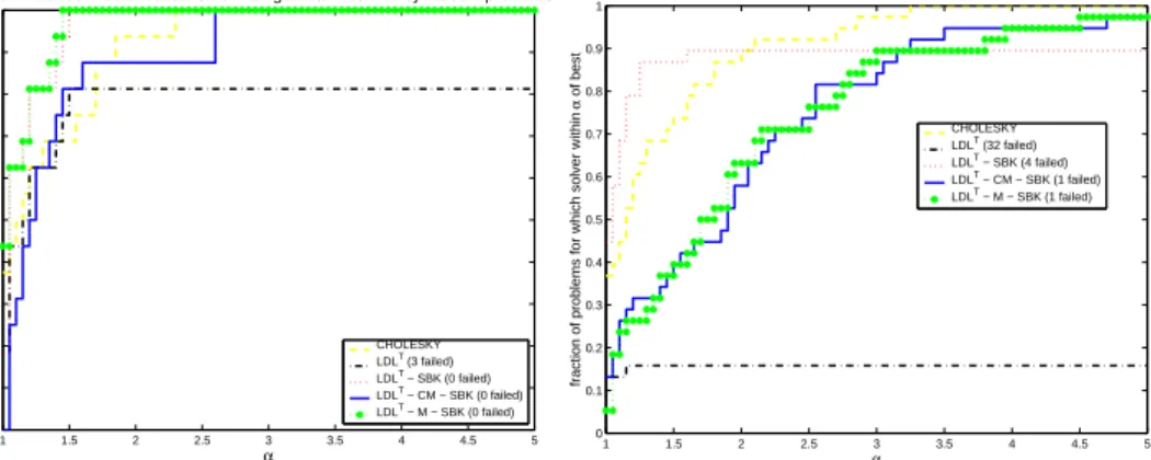
Fig. 5.4. Performance profile CPU time for the analysis for both sets of symmetric indefinite
matrices. 1 1.5 2 2.5 3 3.5 4 4.5 5 0 0.1 0.2 0.3 0.4 0.5 0.6 0.7 0.8 0.9 1
Performance Profile: Factor.CPU − 16 general indefinite symmetric problems
α
fraction of problems for which solver within
α of best CHOLESKY LDLT (3 failed) LDLT − SBK (0 failed) LDLT − CM − SBK (0 failed) LDLT − M − SBK (0 failed) 1 1.5 2 2.5 3 3.5 4 4.5 5 0 0.1 0.2 0.3 0.4 0.5 0.6 0.7 0.8 0.9 1 α
fraction of problems for which solver within
α
of best
Performance Profile: Factor.CPU − 38 augmented indefinite symmetric problems
CHOLESKY LDLT (32 failed)
LDLT − SBK (4 failed)
LDLT − CM − SBK (1 failed)
LDLT − M − SBK (1 failed)
Fig. 5.5. Performance profile CPU time for the numerical factorization for both sets of
sym-metric indefinite matrices.
always shows the performance profiles for the general indefinite systems whereas the right graphic shows profile information for the augmented symmetric indefinite sys-tems.
It is immediately apparent that augmented symmetric indefinite systems are much
harder to solve than general indefinite systems. The method LDLT failed on three
matrices out of 16 general indefinite systems and also on 32 out of 38 augmented sys-tems. This diagonal pivoting method is not reliable and more sophisticated methods must be used. Additionally it is clearly visible that the overall reliability of the
meth-ods LDLT−SBK, LDLT−M−SBK, and LDLT−CM−SBK is generally high and
the absolute CPU time is in the same order of magnitude as that of the CHOLESKY method. This is already a good indication of the robustness and performance of our method. The results also show that weighted graph matchings have a strong influence on the overall performance of the augmented symmetric indefinite systems, where the
method without symmetric matchings LDLT −SBK is superior if it works to the
LDLT −M−SBK, and LDLT−CM−SBK strategies. For the general indefinite
systems there is only a minor difference due to the reason that for almost all systems the permutation produced by the symmetric matchings is identical or very close to
1 1.5 2 2.5 3 3.5 4 4.5 5 0 0.1 0.2 0.3 0.4 0.5 0.6 0.7 0.8 0.9 1
Performance Profile: Nonzeros in L − 16 general indefinite symmetric problems
α
fraction of problems for which solver within
α of best CHOLESKY LDLT (3 failed) LDLT − SBK (0 failed) LDLT − CM − SBK (0 failed) LDLT − M − SBK (0 failed) 1 1.5 2 2.5 3 3.5 4 4.5 5 0 0.1 0.2 0.3 0.4 0.5 0.6 0.7 0.8 0.9 1 α
fraction of problems for which solver within
α
of best
Performance Profile: Nonzeros in L − 38 augmented indefinite symmetric problems
CHOLESKY LDLT (32 failed)
LDLT − SBK (4 failed)
LDLT − CM − SBK (1 failed)
LDLT − M − SBK (1 failed)
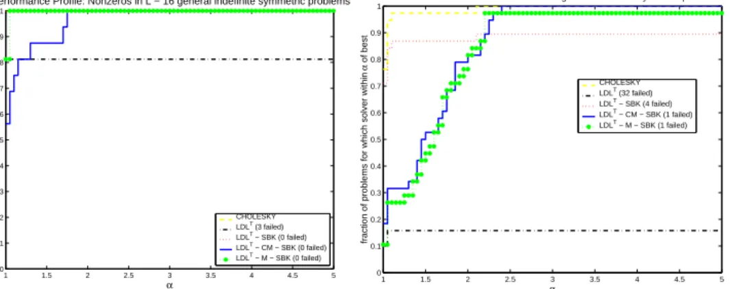
Fig. 5.6. Performance profile for the numbers of nonzeros in the factor L for both sets of
symmetric indefinite matrices.
2 4 6 8 10 12 14 16 10−9 10−8 10−7 10−6 10−5 10−4 10−3 10−2 10−1 100 Matrices
Log Scale of (No. of Pivots / No. of Unknowns)
Perturbed Pivots − 16 general indefinite symmetric problems
LDLT − SBK (0 failed) LDLT − CM − SBK (0 failed) LDLT − M − SBK (0 failed) 5 10 15 20 25 30 35 10−9 10−8 10−7 10−6 10−5 10−4 10−3 10−2 10−1
100 Perturbed Pivots − 38 augmented indefinite symmetric problems
Matrices
Log Scale of (No. of Pivots / No. of Unknowns)
LDLT − SBK (4 failed)
LDLT − CM − SBK (1 failed)
LDLT − M − SBK (1 failed)
Fig. 5.7. Percentage of perturbed pivots for both sets of symmetric indefinite matrices.
the identity. A close examination of the separate analysis, factorize and solution time will reveal this in Figures 5.4 to 5.10.
Figure 5.4 compares the profiles for the analysis. The analysis time for the
meth-ods CHOLESKY, LDLT, and LDLT −SBK are very similar since these methods
do not apply a weighted matching as an additional preprocessing step based on the
numerical values of A during analysis. As a result, these methods have the fastest
analysis time for both sets of indefinite systems. The graph-weighted matchings
meth-ods LDLT−M−SBK, and LDLT−CM−SBK produced a nontrivial permutation
for six general indefinite matricescopter2,dawson5,DIXMAANL,LINVERSE,NCVXBQP1,
SPMSRTLSand for all augmented symmetric indefinite systems. Comparing the
pro-files for LDLT−M−SBK, and LDLT−CM−SBK, we can see the analysis for the
method based in compressed indistinguishable vertices is faster compared to
reorder-ing method based on local modifications. The reason is that LDLT −CM−SBK
constructs a smaller adjacency graph based on compressed block pivots that are
iden-tified during the matching process. The analysis time for theMetis ordering on the
small compressed graph is in all cases smaller compared to theMetisordering on the
original adjacency graph for the LDLT−M−SBK method.
1 1.5 2 2.5 3 3.5 4 4.5 5 0 0.1 0.2 0.3 0.4 0.5 0.6 0.7 0.8 0.9 1
Performance Profile: Solve.CPU − 16 general indefinite symmetric problems
α
fraction of problems for which solver within
α of best CHOLESKY LDLT (3 failed) LDLT − SBK (0 failed) LDLT − CM − SBK (0 failed) LDLT − M − SBK (0 failed) 1 1.5 2 2.5 3 3.5 4 4.5 5 0 0.1 0.2 0.3 0.4 0.5 0.6 0.7 0.8 0.9 1 α
fraction of problems for which solver within
α
of best
Performance Profile: Solve.CPU − 38 augmented indefinite symmetric problems
CHOLESKY LDLT (32 failed)
LDLT − SBK (4 failed)
LDLT − CM − SBK (1 failed)
LDLT − M − SBK (1 failed)
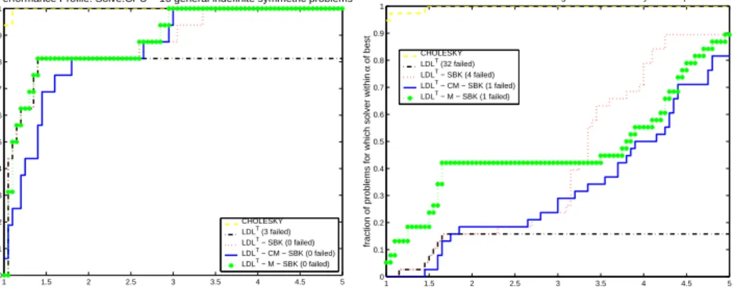
Fig. 5.8. Performance profile CPU time for the solve including iterative refinement for both
sets of symmetric indefinite matrices.
2 4 6 8 10 12 14 16 10−16 10−15 10−14 10−13 10−12 10−11 10−10 Matrix Number
Log Relative Residual
Relative Residual for 16 general indefinite symmetric problems
LDLT − SBK (0 failed) LDLT − CM − SBK (0 failed) LDLT − M − SBK (0 failed) 5 10 15 20 25 30 35 10−16 10−14 10−12 10−10 10−8 10−6 10−4 10−2 100 Matrix Number
Log Relative Residual
Relative Residual for 38 augmented indefinite symmetric problems
LDLT − SBK (4 failed)
LDLT − CM − SBK (1 failed)
LDLT − M − SBK (1 failed)
Fig. 5.9.Accuracy of the relative residual for both sets of symmetric indefinite matrices.
in the factors for all methods. It is remarkable that the LDLT−SBK factorization
method is faster than CHOLESKY for both types of linear systems. This clearly
demonstrates the high performance capabilities of our LDLT−SBK method. When
applying symmetric matchings to the augmented indefinite systems, the factorization is in general about a factor of three slower due to the fact that the resulting factors
require more nonzeros compared to LDLT−SBK. We also see that the LDLT−M−
SBK requires less non-zero entries in the factor compared to LDLT−CM−SBK for
the general indefinite systems.
Now we turn our attention to the numbers of perturbed pivots during factoriza-tion. Figure 5.7 demonstrates that only three of the sixteen general indefinite systems are effected by pivot perturbation. This is different for the augmented indefinite sys-tems, where for most of the systems pivot perturbation occurs during factorization. The Figure 5.7 shows the percentage of perturbed pivots and it can be seen that the additional preprocessing can reduce the occurrence of pivot perturbation by several
orders of magnitude due to the effective initial construction of 1×1 and 2×2 cycles
during the analysis. This increases the factorization time by about a factor of three, but it also adds reliability that might be needed in various applications.
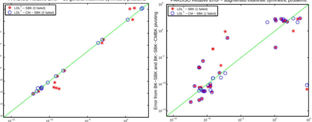
10−15 10−10 10−5 100 10−16 10−14 10−12 10−10 10−8 10−6 10−4 10−2 100 102
PARDISO Relative Error − 16 general indefinite symmetric problems
Error from LDLT solver with MA27 (BK pivoting)
Error from BK−SBK and BK−SBK−CMBK pivoting
LDLT − SBK (0 failed) LDLT − CM − SBK (0 failed) 10−15 10−10 10−5 100 105 10−15 10−10 10−5 100
105 PARDISO Relative Error − augmented indefinite symmetric problems
Error from LDLT with MA27 solver (BK pivoting)
Error from BK−SBK and BK−SBK−CMBK pivoting
LDLT − SBK (1 failed) LDLT − CM − SBK (1 failed)
Fig. 5.10.Comparison of relative error withLDLT−CM−SBK,LDLT−SBKand Ma27for
both sets of symmetric indefinite matrices.
mentioned in 5.2, we perform two steps of an iterative refinement method if any pivot
perturbation has been encountered during factorization for the methods LDLT −
SBK, LDLT −M−SBK, and LDLT−CM−SBK. It is clear that the solve step
is affected by this strategy and the figures demonstrate that the influence is higher for the augmented linear systems. There might be a different termination criterion e.g. based on the backward error as described in [24], but have have not further investigated this.
Figure 5.9 and Figure 5.10 show the accuracy for all factorization pivoting meth-ods and all general and augmented indefinite systems. Figure 5.9 compares the scaled
residual (kb−Axk/(kAk kxk+kbk)). A residual in the order of 1 indicates a failure
of the method. It can be seen that the residual is for most of the general indefinite
systems less than 10−14. For the augmented indefinite systems the LDLT−M−SBK
and LDLT−CM−SBK methods produce often residual close to machine precision.
The LDLT−SBK residuals are often a bit larger and for four systems, the
residu-als are in the order of 10−10. However, the general conclusion is that even in the
presence of large pivots, the iterative refinement can effectively recover the loss of
accuracy during factorization. Figure 5.10 assesses the accuracy of our LDLT−SBK
and LDLT−CM−SBK methods. The Figure plots the relative errorkx−1kfrom
both methods versus the relative error from a pivoting method that uses 1×1 and
2×2 Bunch and Kaufman pivoting for the complete matrix. In particular we selected
Ma27from [19] as a direct solver for thex-axis in the Figure. A dot on the diagonal
means that the two errors were the same, a dot above means thatMa27is more
accu-rate, and a dot below the diagonal means that the LDLT−SBK and LDLT−CM−SBK
methods are more accurate. Please note that it is not possible to solve some of the
systems withMa27and we only report the error for those matrices whereMa27did
not fail [17]. As already mentioned most of the augmented systems are much harder to solve than the general indefinite systems but it can be concluded from these figures
that the error of Ma27 and the LDLT−SBK and LDLT−CM−SBK methods in
Pardisoare of the same order.
5.6. Numerical results for interior point optimization matrices. In
Ta-bles 5.11 and 5.12 and Figure 5.13 we report the performance of Pardisousing the
whole set consists of 57 matrices of increasing size and can be found at [5]. We use a subset of 16 matrices, which was selected to include the hard to solve examples, as well as to give an impression of scalability and the robustness of the methods.
Therefore, matrices from the whole range were picked. The core step of the Ipopt
optimization algorithm is a damped Newton iteration, where in each step a modified, symmetrized linear system of the form
A= W + Σ +δwI B BT −δ cI (5.4)
is solved. In our examples, the upper left block A11 = W + Σ +δwI is a diagonal
matrix, B is of full rank, and δc is set to 10−8. We also refer to Ma27 since this
solver is used within this package to solve the symmetric indefinite linear systems.
There might be other packages fromHslthat are more appropriate for Ipopt. The
focus on this section is mainly to demonstrate the competitiveness of our innovative
LDLT−SBK and LDLT−CM−SBK methods to conventional approaches4.
The Table 5.11 shows the name of theIpoptmatrices, and the numbers of positive
and negative eigenvalues. It can be seen that all the matrices are very indefinite and in general hard to solve. The Table also shows the time in seconds for the analysis, factorization and solution. It can be seen that for larger examples the factorization
speedup ofPardisotoMa27is in the order of sixty, whereas solve and analysis time
are similar due to the fact that two steps of iterative refinement are used inPardiso
in cases if a pivot perturbation has been encountered.
Table 5.12 shows the numbers of nonzeros in the factors and the total memory requirement for both methods. The total memory requirement consists of the main memory for the factors and the main memory for additional data structures that the solver consumes during the complete solution process. It can be seen that the
Ma27 was not able to factorc-bigin our 32-bit environment due to high memory
consumption.
Finally, the relative errorkx−1kof both methods versusMa27is demonstrated
in Figure 5.13. As in Figure 5.10, a dot on the diagonal means that the two errors
were the same, a dot above means that Ma27 is more accurate, and a dot below
the diagonal means that the LDLT −SBK and LDLT −CM−SBK methods are
more accurate. We do not list the residuals here since we noticed that both solvers
always produced residuals close to machine precision. For allIpoptmatrices our fast
LDLT−SBK and LDLT−CM−SBK methods produced similar errors asMa27.
Finally, we evaluate the runtime of each step of the LDLT−CM−SBK in Figure
5.14 for all symmetric indefinite systems (general, augmented, Ipopt). The Figure
5.14 shows the fraction of runtime for the computation of the symmetric matching, the reordering and the solution including iterative refinement with respect to the time
for the numerical factorization. For large enough examples, theLDLT factorization
dominates all other steps. The computation of the matching is for all matrices smaller
than the analysis time except for the matrixBOYD2from the test set in Table 5.2. We
noticed that our matching codemps required a disproportionate amount of time for
matrixBOYD2, which seems to be due to a large number of dense rows in this matrix.
6. Conclusions. This paper demonstrates the effectiveness of various new
piv-oting methods for sparse symmetric indefinite systems. As opposed to many existing
4
Detailed comparisons of sparse direct linear solver for symmetric indefinite systems can be found in [16, 17, 32].
Matrix pardiso ma27
name n+ n− analysis factor solve analysis factor solve
c-20 1’621 1’300 0.05 0.01 .002 0.01 0.01 .001 c-22 2’130 1’662 0.08 0.01 .003 0.01 0.02 .002 c-27 2’621 1’942 0.08 0.01 .003 0.01 0.02 .002 c-30 2’823 2’498 0.21 0.01 .005 0.08 23.8 .033 c-33 3’526 2’791 0.12 0.02 .006 0.10 0.04 .004 c-40 5’477 4’464 0.20 0.02 .009 0.20 12.8 .031 c-42 5’930 4’541 0.27 0.05 .012 0.11 0.06 .006 c-55 19’121 13’659 1.47 5.64 0.11 0.78 158. 0.18 c-58 22’461 15’134 1.80 3.69 0.10 1.30 167. 0.18 c-62 25’158 16’573 2.01 13.5 0.20 1.72 863. 0.56 c-68 36’546 28’264 2.70 14.7 0.21 2.31 612. 0.38 c-70 39’302 29’622 3.07 4.20 0.14 0.89 90.3 0.16 c-71 44’814 31’824 3.83 47.6 0.41 3.30 1219 0.70 c-72 47’950 36’114 3.50 2.96 0.15 0.92 71.2 0.17 c-73 86’417 83’005 28.1 2.04 0.18 198. 1.62 0.08 c-big 201’877 143’364 18.9 214. 1.40 30.1 — —
Fig. 5.11. Comparison of two sparse direct linear solver Pardiso and Ma27 using default options for a subset of the IPOPT interior point optimization matrices. The table shows time in seconds for analysis, factorization and solve. n+andn−show the number of positive and negative
eigenvalues.
pivoting methods, LDLT−SBK uses both dynamical and static pivoting within the
numerical factorization, resulting in a fast factorization algorithm. We demonstrated numerical stability of the algorithm and also showed that a high performance imple-mentation is feasible for this algorithm. Our goal is to have sparse symmetric
indef-inite factorization as fast and reliable as sparse Cholesky factorization andPardiso
is competitive and faster than any other recent high-performance sparse symmetric indefinite code as shown in [16, 32].
Another benefit that adds a new level of reliability is the use of symmetric
weighted matchings as shown with the LDLT−CM−SBK and LDLT−M−SBK
methods. The numerical experiments show that the additional effort of symmetric
weighted matchings for producing good initial 1×1 and 2×2 pivots during the
anal-ysis is not always required. However, these two methods add an additional level of reliability without significantly decreasing the performance of the solver. For a large
number of real-world examples, LDLT−CM−SBK and LDLT−M−SBK reorderings
are capable of providing a feasible pivoting order for the factorization, while the cost of this preprocessing step is often negligible.
In addition, our methods open new possibilities to achieve scalability for symmet-ric indefinite factorization on parallel architectures, since similar data structures and communication patterns as in sparse Cholesky can be exploited.
Acknowledgments. The authors thank Jennifer Scott for discussions during the
surveys and providing the matrices from [17], and Andreas W¨achter for the Ipopt
interior point optimization matrices. We also thank Michael Hagemann for assisting in the implementation of the cycle matchings.
Matrix pardiso ma27
name nnz inL memory nnz inL memory
c-20 31’236 1 37’978 1 c-22 43’044 1 60’487 2 c-27 40’615 1 71’616 2 c-30 43’784 2 1’463’166 23 c-33 61’372 2 103’453 3 c-40 68’830 4 1’398’151 21 c-42 125’161 5 157’369 6 c-55 3’567’897 36 7’706’392 346 c-58 2’605’211 30 7’424’529 296 c-62 6’760’217 64 24’486’396 640 c-68 5’584’384 57 16’302’275 494 c-70 3’302’552 42 6’181’749 243 c-71 13’768’053 126 30’270’388 1’474 c-72 2’977’867 45 6’518’717 208 c-73 2’085’753 71 1’750’645 95 c-big 39’032’735 365 — >2 GByte
Fig. 5.12.Comparison of the direct linear solver PardisoandMa27using default options for a subset of the IPOPT interior optimization matrices. The table shows the numbers of nonzero in the factorLand the total memory requirement in MByte.
10−13 10−12 10−11 10−10 10−9 10−8 10−13 10−12 10−11 10−10 10−9
10−8 PARDISO Relative Error − general indefinite symmetric IPOPT problems
Error from LDLT solver with MA27 ( BK pivoting )
Error from BK−SBK and BK−SBK−CMBK pivoting
LDLT − SBK (0 failed)
LDLT − CM − SBK (0 failed)
Fig. 5.13.Comparison of relative error withLDLT−CM−SBK,LDLT−SBKand Ma27for
general symmetric indefiniteIpoptmatrices.
[1] J.O. Aasen. On the reduction of a symmetric matrix to triagonal form.BIT, 11:233–242, 1971.
[2] C. Ashcraft. Compressed graphs and the minimum degree algorithm. SIAM Journal on
Sci-entific Computing, 16:1404–1411, 1995.
[3] C. Ashcraft, R.G. Grimes, and J.G. Lewis. Accurate symmetric indefinite linear equation
solvers. SIAM J. Matrix Analysis and Applications, 20(2):513–561, 1999.
[4] C.C. Ashcraft and R.G. Grimes. The influence of relaxed supernode partitions on the
multi-frontal method. ACM Trans. Math. Softw., 15(4):291–309, 1989.
[5] Basel Sparse Matrix Collection. http://computational.unibas.ch/cs/scicomp/matrices.
[6] M. Benzi, J.C. Haws, and M. Tuma. Preconditioning highly indefinite and nonsymmetric
matrices. SIAM J. Scientific Computing, 22(4):1333–1353, 2000.
[7] J.R. Bunch and L. Kaufmann. Some stable methods for calculating inertia and solving
sym-metric linear systems. Mathematics of Computation, 31:162–179, 1977.
10−2 10−1 100 101 102 103 10−3 10−2 10−1 100 101 102
103 CPU statistics for all symmetric indefinite systems
LDLT−CM−SBK Factorization Runtime in Seconds
Fraction of LDL
T−CM−SBK Factorization Runtime
Symmetric Weighted Matching Reordering Solve and Iterative Refine BOYD2
Fig. 5.14.The runtime of theLDLT−CM−SBKmethod versus other steps (computation of the
matching, reordering and solution with iterative refinement) for all symmetric indefinite systems.
SIAM J. Numerical Analysis, 8:639–655, 1971.
[9] E. D. Dolan and J.J. Mor´e. Benchmarking optimization software with performance profiles.
Mathematical Programming, 91(2):201–213, 2002.
[10] I. S. Duff and J. R. Gilbert. Maximum-weighted matching and block pivoting for symmetric
indefinite systems. InAbstract book of Householder Symposium XV, pages 73–75, June
17-21 2002.
[11] I. S. Duff and J. Koster. The design and use of algorithms for permuting large entries to the
diagonal of sparse matrices. SIAM J. Matrix Analysis and Applications, 20(4):889–901,
1999.
[12] I. S. Duff and J. Koster. On algorithms for permuting large entries to the diagonal of a sparse
matrix.SIAM J. Matrix Analysis and Applications, 22(4):973–996, 2001.
[13] I. S. Duff and S. Pralet. Strategies for scaling and pivoting for sparse symmetric indefinite problems. Technical Report TR/PA/04/59, CERFACS, Toulouse, France, 2004.
[14] I.S. Duff, A.M. Erisman, and J.K.Reid. Direct methods for sparse matrices. Oxford Science
Publications, 1986.
[15] I.S. Duff and S. Pralet. Symmetric weighted matching and application to indefinite multifrontal
solvers. InSIAM Workshop on Combinatorial Scientific Computing (CSC04), February
25-27, 2004.
[16] N.I.M. Gould, Y. Hu, and J.A. Scott. A numerical evaluation of sparse direct solvers for the solution of large sparse, symmetric linear systems of equations. Technical report, Rutherford Appleton Laboratory, 2004. to appear.
[17] N.I.M. Gould and J.A. Scott. A numerical evaluation of HSL packages for the direct solution of large sparse, symmetric linear systems of equationss. Technical Report RAL-2003-019, RAL, 2003.
[18] A. Gupta and L. Ying. On algorithms for finding maximum matchings in bipartite graphs. Technical Report RC 21576 (97320), IBM T. J. Watson Research Center, Yorktown Heights, NY, October 25, 1999.
[19] Harwell Subroutine Library, AEA Technology, Harwell, Oxfordshire, England catalogue of sub-routines, 2002.
[20] J.C. Haws and C.D. Meyer. Preconditioning KKT systems. Numerical Linear Algebra with
Applications. Accepted, in press.
[21] N.J. Higham. Accuracy and Stability of Numerical Algorithms. SIAM Press, Philadelphia,
2002. Second edition.
[22] G. Karypis and V. Kumar. A fast and high quality multilevel scheme for partitioning irregular
graphs. SIAM J. Scientific Computing, 20(1):359–392, 1998.
[23] H. W. Kuhn. The hungarian method for solving the assignment problem. Naval Res. Logist.
Quart, (2):83–97, 1955.
[24] X. S. Li and J. W. Demmel. SuperLU DIST: A scalable distributed-memory sparse direct solver
for unsymmetric linear systems.ACM Trans. Math. Softw.Accepted, in press.
[25] X.S. Li and J.W. Demmel. A scalable sparse direct solver using static pivoting. InProceeding
Texas, March 22-34,1999.
[26] O. Meshar and S. Toledo. An out-of-core sparse symmetric indefinite factorization method.
ACM Trans. Math. Softw. Submitted. Under revision.
[27] M. Olschowka and A. Neumaier. A new pivoting strategy for gaussian elimination. Linear
Algebra and its Applications, 240:131–151, 1996.
[28] S. R¨ollin and O. Schenk. Maximum-weighted matching strategies and the application to
symmetric indefinite systems. In Workshop on State-of-the-Art in Scientific Computing
PARA’04, June 20-23 2004.
[29] O. Schenk and K. G¨artner. Solving unsymmetric sparse systems of linear equations with
PARDISO. Journal of Future Generation Computer Systems, 20(3):475–487, 2004.
[30] O. Schenk, K. G¨artner, and W. Fichtner. Efficient sparse LU factorization with left-right
looking strategy on shared memory multiprocessors.BIT, 40(1):158–176, 2000.
[31] O. Schenk, S. R¨ollin, and A. Gupta. The effects of unsymmetric matrix permutations and
scalings in semiconductor device and circuit simulation.IEEE Transactions On
Computer-Aided Design Of Integrated Circuits And Systems, 23(3), 2004.
[32] J.A. Scott. A numerical evaluation of sparse solvers for the direct solution of large sparse
sym-metric linear systems”. InTalk at CERFACS Sparse Days Meeting, June 2004. Available
atftp://ftp.numerical.rl.ac.uk/pub/talks/sct.cerfacs04.pdf.
[33] A. W¨achter and L. T. Biegler. On the implementation of a primal-dual interior point filter
line search algorithm for large-scale nonlinear programming. Technical report, IBM T. J. Watson Research Center, Yorktown, NY, March 2004.