Chapman University Chapman University
Chapman University Digital Commons
Chapman University Digital Commons
Business Faculty Articles and Research Business
3-26-2019
Dynamic Pricing with Fairness Concerns and a Capacity
Dynamic Pricing with Fairness Concerns and a Capacity
Constraint
Constraint
Matthew SeloveFollow this and additional works at: https://digitalcommons.chapman.edu/business_articles Part of the Business Administration, Management, and Operations Commons, Economic Theory Commons, Other Business Commons, and the Sales and Merchandising Commons
Dynamic Pricing with Fairness Concerns and a
Capacity Constraint
∗
Matthew Selove
†March 12, 2019
Abstract
Although some firms use dynamic pricing to respond to demand fluctuations, other firms claim that fairness concerns prevent them from raising prices during periods when demand exceeds capacity. This paper explores conditions in which fairness concerns can or cannot cause shortages. In our model, a firm announces a price policy that states its prices during high and low demand, and customers must travel to a venue to learn the current price. We show that the interaction of fairness concerns with travel costs can cause the firm to set stable prices, which leads to shortages during high demand. However, if the firm is able to inform customers about the current price before they incur any travel costs, then dynamic pricing with no shortages is optimal even with strong fairness concerns.
∗Helpful comments were provided by Anthony Dukes, Jeanine Mikl´os-Thal, Daniel Mochon,
Cristina Nistor, Mohammad Zia, and seminar participants at Chapman, Florida, UC Irvine, and the 2019 Marketing Theory Symposium. Peter Selove inspired me to work on this project.
1
Introduction
Managers often claim that fairness concerns compel them to maintain stable prices, even during periods when their demand exceeds their capacity. Until recently, Disney theme parks had ticket prices that stayed constant throughout the year, partly because executives “thought it would be unfair to charge different prices for what some would see as the same product” (Economist 2016). Disney did not raise ticket prices even during times of year when their parks consistently reached maximum capacity, so they had to close their gates to new customers (Martin 2014). Similarly, the commissioner of the National Basketball Association once stated that NBA teams did not set higher ticket prices for more popular games than for less popular games because doing so “raises questions about the fairness of your pricing” (Lefton and Lombardo 2003). Teams did not raise prices even for games they knew would have ticket sell-outs that left many fans unable to purchase (Rovell 2001).
However, some organizations that previously maintained constant prices have begun to vary prices over time. Disneyland has adopted a new policy in which ticket prices are higher during the most popular days to visit the park (Fritz 2016). Likewise, NBA teams and other professional sports teams have started setting higher ticket prices for more popular games than for less popular games (Drayer et al. 2012; Shapiro et al. 2016).
Academic researchers, consultants, and business journalists continue to debate how fairness concerns should affect firms’ price policies. Previous academic research has shown that many customers think it is unfair for a firm to raise prices during a temporary spike in demand (Kahneman et al. 1986; Bolton et al. 2003). These papers imply firms should maintain stable prices during demand spikes, even during shortages. On the other hand, the basic theory of supply and demand shows that, when demand exceeds capacity, price increases lead to higher profits and more efficient
allocation of resources (Feeney 2014; Weiner 2014; Mohammed 2015). Furthermore, customers who consider these price increases unfair can simply choose not to purchase during peak demand. Such arguments imply that fairness concerns should not lead to shortages.
The current paper develops a formal model to derive conditions in which fairness concerns can or cannot cause shortages. In our model, a firm sets a price policy that specifies its prices during high and low demand. In each period, customers in the market are uncertain whether demand is currently high or low. For example, news stories reported that many customers did not anticipate Disneyland’s high demand on Christmas Day until they had driven to the park (Martin 2014). Because they do not know the current demand level, customers must incur the cost of traveling to a venue (where the product is sold) to learn the current price. Under variable pricing, customers with fairness concerns anticipate that, if they travel then buy when prices are high, they will experience disutility both from the direct effect of a higher price and also from the unfairness of knowing they are paying more than customers who traveled when demand was low. To avoid imposing this disutility on its customers, a profit-maximizing firm may want to set stable prices, even if there are shortages during high demand.
However, if the firm can reveal the current price to customers before they travel, then customers with fairness concerns and low valuations can decide to travel only during low demand, when prices are low. In this case, the firm uses dynamic pricing with no shortages, even in the presence of strong fairness concerns. Thus, shortages occur in the model only if the firm does not have a low-cost way to reveal the current price to customers before they incur travel costs.
Our results provide one possible explanation for why some industries have adopted variable pricing, whereas others have not. As the Internet reduces communication
costs, some firms can easily provide advance price information to customers. For example, Disneyland’s website now states one-day admissions prices for each day of the current calendar year, with each day designated as “value,” “regular,” or “peak” pricing.1 If such communications allow customers to learn the current price before they drive to the park, then our results imply the firm should use variable pricing, which prevents shortages.
On the other hand, some firms maynot be able to provide customers with advance price information if they used variable pricing. For example, because weather forecasts are imprecise, a firm’s predictions of its own future price changes based on weather conditions would also be imprecise. Therefore, our results imply retail stores might want to maintain constant prices for umbrellas even though many stores sell out of umbrellas when it rains (Rogers 2016).2 Similarly, because predicting the future temperature and informing customers about a vending machine’s future prices may be costly or impractical, our results help explain why Coke abandoned a technology that would raise prices in its vending machine during high temperatures (Leonhardt 2005).3
Section 2 discusses related literature. Section 3 presents the formal model. Section 4 presents conclusions. The appendix contains formal proofs of all results.
1Prices are available at https://disneyland.disney.go.com/tickets/. As another example, Uber
sometimes warns customers about periods with unusually high surge prices. On New Year’s Eve of 2016, Uber released this statement: “On this busy night, fares will be the highest between midnight and 3am as people head home for the night” (Haydu 2016).
2We interviewed a Disneyland executive who said that stores in their theme park often have
stockouts of umbrellas when it rains. He said they would not consider raising the price of umbrellas when it is raining because of the potential backlash from customers who would consider such price increases unfair.
3The CEO of the Coca Cola Company once proposed vending machines that would automatically
raise the price of drinks when the temperature was hot. After complaints that this price policy would represent “gouging” and “exploitation” of customers, the company canceled its plans to vary prices based on temperature (Leonhardt 2005).
2
Related Literature
Kahneman et al. (1986) make an informal argument that fairness concerns can lead to shortages. They present survey results showing that most people would consider it unfair, for example, for a firm to raise the price of snow shovels after a snowstorm. The authors then hypothesize that, if firms engage in such price “gouging,” customers punish the firm by reducing their purchases during subsequent periods that have lower demand levels. Rotemberg (2005) develops a formal model in which customers punish a firm if it engages in unfair pricing. Our paper demonstrates a different mechanism for how fairness concerns can cause shortages. Fairness concerns in our model do not involve desire for punishment or enforcement of social norms. Rather, customers derive disutility from paying a higher price than others, and raising prices during peak demand does not lead to any punishment in subsequent periods if customers know in advance the firm’s price and demand level in each period. Customer uncertainty about demand is a key element of how fairness concerns cause shortages in our model. Lab experiments have shown that people may reject offers they perceive as unfair, even if accepting the offer would increase their own monetary payoff (e.g., Hoffman et al. 1994; Camerer and Thaler 1995). Field experiments have also shown that customers who pay a high price and then observe others paying a lower price for the same item are less likely to purchase from the company in the future, which is consistent with these customers deriving disutility from paying a higher price than others do (Anderson and Simester 2010). Motivated by such experimental findings, Fehr and Schmidt (1999) develop a model of fairness in which each player’s utility depends on his own payoff and the difference between this payoff and that of other players. We use this utility model as the basis for incorporating fairness into our model. Previous research has used a similar approach to incorporate fairness into models of channel pricing (Cui et al. 2007), third-degree price discrimination
(Englmaier et al. 2012; Okada 2014), pricing with customer recognition (Li and Jain 2016), pricing with private information about the firm’s costs (Guo 2015; Guo and Jiang 2016), and pay-as-you-wish pricing (Chen et al. 2017). These earlier models do not involve shortages or rationing in equilibrium. The new aspect of our paper is to develop a formal model of how fairness concerns in the style of the Fehr and Schmidt (1999) model can lead to rationing.
Under alternative assumptions, our model could generate shortages even without
fairness concerns. In particular, if we assumed there was a negative correlation between a customer’s valuation and the change in his probability of being in the market during high versus low demand periods, as in the model by Gilbert and Klemperer (2000), then rationing could occur in equilibrium even without fairness concerns. However, in the case of entertainment attractions like Disneyland, this alternative explanation for rationing would require that tourists (who are in the market primarily during peak demand periods) have alower per-visit valuation than local customers (who are in the market throughout the year), which is the opposite of what we would normally expect. Our results show that fairness concerns provide a different explanation for shortages, which does not depend on average valuation of customers in the market decreasing during peak demand.
Previous theoretical research has shown firms may want to restrict capacity to induce high valuation customers to buy during an early period with high prices and thus avoid possible regret or disappointment from being unable to purchase later (Liu and Shum 2013; Nasiry and Popescu 2012; Ozer and Zheng 2016). In these models, rationing increases profits by creating uncertainty about purchase availability for customers who wait to purchase at lower prices. Our paper provides a different explanation for rationing. The firm in our model does not intentionally restrict its capacity, and in fact, its profits increase as its capacity grows.
Previous research has studied other reasons firms might set prices low enough to require rationing their product. Rationing can occur if customers desire a product more as a result of other customers consuming it (Becker 1991), if price adjustment is costly (Levy et al. 1997), if a firm sets prices before learning demand for the period (Su 2010). We demonstrate a new explanation for rationing, in particular, that it can result from the interaction of customers’ uncertainty about demand and their disutility from paying a higher price than others.
Wernerfelt (1994) develops a model in which price advertising induces customers to incur the cost of inspecting a good. Similarly, in the current paper, the firm announces a price policy to induce customers to incur the cost of travel. We show how the optimal price policy (the choice of fixed versus variable pricing) depends on the firm’s ability to inform customers with fairness concerns about the current price before they incur travel costs.
3
Model
A monopolist can sell a product over an infinite number of periods, denoted by
t∈ {1,2,3, . . .}. There is a mass D of potential customers with product valuations uniformly distributed on [0, V]. Each customer can purchase at most one unit in each period, but can purchase in multiple different time periods. For analytical simplicity, we assume that a customer’s purchase decision in one period does not affect his valuation in subsequent periods. In contrast with dynamic pricing models in which each customer purchases at mostonce (e.g., Nasiry and Popescu 2012), in our model the firm seeks to maximizes profits from customers who make repeat purchases.
Each period has probability H of having high demand and (1− H) of having low demand, with the demand state independent across time periods. During high
demand periods, a mass DH of the customers are available potentially to purchase
the product, and during low demand periods, a mass DL of the customers are
potentially available, where 0 < DL < DH ≤ D. For example, in each period,
some potential customers consider traveling to a vacation destination, whereas others donot consider traveling to the destination (at any price) because they are busy with other professional or personal obligations during that period. The choice of which particular customers are in the market is independent across periods. There is a proportional shift in the demand curve between high and low demand periods, that is, there is no correlation between a customer’s valuation and the difference in his likelihood of being in the market during high versus low demand.
Before the fist period, the firm announces a price policy that specifies unit prices
PH and PL it will charge during high demand and low demand periods, respectively,
where PH ≥0 and PL ≥0. Customers learn the firm’s price policy as a result of its
announcement. The basic insights of our model would still hold if customers learned the price policy in other ways, for example, by reading news stories about the firm’s dynamic price policy or by learning about this policy through personal experience with their first few purchases. We initially assume the firm’s announcement is binding, but we relax this assumption in section 3.3 and allow the announcement to be “cheap talk,” and we derive conditions in which reputation effects compel the firm not to deviate from its announced price policy.
After learning the firm’s price policy, in each period customers in the market decide whether to incur cost c to travel to the venue where the product is sold to learn the price for the current period, where 0 ≤ c < V. We later present a model extension in section 3.4 that separates search and travel costs, so customers can search for the current price before deciding whether to travel to the entertainment venue (for example) or travel directly to the venue without searching first.
Customers who travel to the venue then have the option to attempt to purchase the product. The firm has a capacity constraint, so that in each period it can serve at most K customers, whereK >0. If the number of customers who attempt to buy exceeds capacity, thenK of the customers are randomly selected to buy the product, with all of the customers who attempt to buy having equal chances of being chosen. Customers maximize their expected utility, with fairness concerns modeled in a similar manner to the model of customer recognition by Li and Jain (2016). A customer with valuation vi derives utility 0 if he does not travel to the venue, −c if
he travels and then decides not to purchase or makes a failed purchase attempt, and
vi−c−Pt−α(Pt−min(PL, PH)) if he purchases at any pricePt≥min(PL, PH), where
α ≥ 0.4 The constant α reflects the disutility customers experience from paying a higher price than others. One interpretation is this term reflects inequity aversion, as in Fehr and Schmidt (1999). Another interpretation is customers who pay higher prices than others suffer transaction disutility, as in Thaler (1985). The particular functional form of this disutility is not essential for our findings. The important aspect of this utility function is that price dispersion across periods reduces the utility of customers who purchase in the high price condition.5
All production costs are normalized to zero, and the firm maximizes expected discounted profits, with discount factor δ, where 0< δ <1.6
4In our base model in section 3.1, price is always equal to one of the firm’s announced prices,
PLor PH, but the model extension in section 3.3 allows the firm to set different prices. We assume
customers derive utilityvi−c−Pt from purchasing at pricePt<min(PL, PH), although the firm
never has an incentive to deviate to a price below its minimum announced price.
5The model of inequity aversion by Fehr and Schmidt (1999) implies that price dispersion would
alsodecreasethe utility of customers in the low price condition who feel bad about inequity, whereas the model of transaction utility by Thaler (1985) implies price dispersion wouldincrease the utility of those in the low price condition who feel good about receiving a favorable deal. However, both models imply that the effect on customers in the high price condition is greater in absolute value than the effect on those in the low price condition. In the interest of parsimony, and similar to the model by Li and Jain (2016), we include only the effect on those in the high price condition.
6In our base model in section 3.1, the discount factor does not affect equilibrium outcomes, but
in the extension in section 3.3, the firm’s discount factor helps determine whether its non-binding price policy announcement is sustainable in equilibrium.
To summarize, the firm first announces a price policy that specifies PL and PH,
and in each period t the game timing is as follows:
1. Nature determines the demand state and the set of customers who are available in the market. The firm automatically sets its price according to its announced policy for the given demand state. Customers do not observe the current demand state or price.
2. Customers who are in the market decide whether to incur the cost to travel to the venue where the product is sold.
3. Customers who traveled to the venue learn the current price and have the option to make a purchase attempt. If there is excess demand, then the product is rationed. Payoffs for the period are realized.
3.1
Results
We first characterize customer behavior in response to any given price policy, and we then characterize the profit-maximizing price policy for the firm.
To decide whether to travel to the venue, customers need to form beliefs about the success probability for purchase attempts in each demand state, which depends on the number of other customers who attempt to purchase. In each period, the number of customers who attempt to purchase depends on the number of customers available in the market (based on the high or low demand state), the fraction of those customers in the market who then travel to the venue, and the fraction of customers at the venue who then attempt to purchase. Customers form beliefs about each of these variables based on rational expectations.
A customer in the market does not initially observe the demand state, but he knows that he himself is in the market, which provides some information about
de-mand. In particular, given prior probabilityH of high demand, a potential customer who observes that he is in the market updates his belief about the probability of the current state having high demand toHb, according to Bayes’ rule:
b
H = HDH
HDH + (1−H)DL
(1) For each demand state, customers form beliefs about the probability they will be able to purchase. Customers also anticipate the utility they would derive from purchasing given their valuation, the price, and possible disutility from unfairness because of price variation. A customer with valuation vi will incur the cost to travel
if the following condition holds:7
b
HSH max[vi−PH −α(PH −PL),0] + (1−Hb)SLmax[vi−PL,0]≥c (2)
where SH and SL are the probability that a purchase attempt succeeds during high
and low demand, respectively. The left side of this equation reflects the expected value to a customer with valuation vi of traveling to the venue.
In equilibrium, customers’ beliefs about success probabilities in each demand state must be accurate given the set of customers who travel. Let v∗ denote the lowest valuation for which customers travel. We will refer to the customer with valuationv∗
as the “marginal customer.” Demand in period tdepends on the maximum ofv∗ and the period’s pricePt, and if prices are not the same in all periods, it is possible forPt
to be either above or below v∗. We can compute the success probabilities as follows:
SH(v∗) = min KV DH(V −max[(PH +α(PH −PL)), v∗]) ,1 (3) 7We have stated this condition, and the following derivations of customer behavior, for the case
in which PH ≥ PL, which is true in equilibrium. In principle, our model also allows PL > PH,
in which case an analogous condition must be satisfied for a customer with valuation vi to learn
SL(v∗) = min KV DL(V −max[PL, v∗]) ,1 (4) These equations represent success probabilities based on the number of people who travel to the venue and make purchase attempts for a given value ofv∗. Note thatSH
and SL are continuous and weakly increasing functions of v∗, and both functions are
equal to one for any v∗ sufficiently close to V. Intuitively, if fewer customers travel, purchase attempts have a higher success probability.
If we insert vi =v∗ into (2), we see that, in equilibrium, the marginal customer’s
valuation must satisfy:
b
HSH(v∗) max[v∗−PH −α(PH −PL),0] + (1−Hb)SL(v∗) max[v∗−PL,0] =c (5)
The left side of (5) is strictly less thancforv∗ = 0, continuous and weakly increasing in v∗, and strictly greater than c for v∗ = V if prices are low enough to induce some customers to travel.8 Thus, for any given price policy, equilibrium customer behavior is characterized by a unique value ofv∗ that solves (5), for which customers with valuations exceeding v∗ travel and then attempt to purchase if their valuation exceeds the period’s price. When this equation holds, customers’ travel behavior is based on correct beliefs about their success probability given the probability of high demand and given the set of customers who travel in each demand state.
For a given price policy (PH, PL), we can computev∗ as described above, and the
firm’s quantity sold during each high-demand period,QH, quantity sold during each
low-demand period, QL, and expected profits in each period, E[πt], are as follows:
QH = min DH(V −max[PH +α(PH −PL)), v∗]) V , K (6) 8Profit-maximizing prices must induce customers with the highest valuation to travel if the success
probability is one. In particular, prices must satisfy (2) for vi = V, SH = 1, andSL = 1, or no
QL= min DL(V −max[PL, v∗]) V , K (7) E[πt] =HPHQH + (1−H)PLQL (8)
In general, there are three types of price policies the firm can use: variable prices (PH > PL) with no rationing; constant prices (PH = PL) with no rationing;
and constant prices (PH = PL) with prices low enough to require rationing during
high demand.9 Because the marginal customer’s valuation, v∗, depends on fairness
disutility during peak demand, and also depends on the purchase success probabilities (which depend on v∗ in a nonlinear manner), it is not generally possible to derive simple close-form expressions for profits under each type of policy. We instead derive sufficient conditions that ensure rationing either does or does not occur in equilibrium. We first show that, if customers do not have fairness concerns, then the firm sets prices such that all purchase attempts are successful, and rationing does not occur.
Proposition 1. If customers do not have fairness concerns (α = 0), there is no
rationing in equilibrium.
Intuitively, if customers do not have fairness concerns, then reducing PH until
shortages occur is not the most profitable way to encourage customers with a given valuation to travel. It would be more profitable to reduce PL to provide the same
expected utility to the marginal customer, that is, to generate the same value of v∗. We next show that, if customers have no travel costs, then in this case as well, no rationing occurs in equilibrium.
Proposition 2. If customers have no travel costs (c = 0), there is no rationing in equilibrium.
9Another feasible strategy would be to set prices that vary across periods, with rationing during
high demand. However, we show in the proof of Lemma 2 that this strategy is always dominated by one of the other strategies.
The intuition for this result is the following. If c = 0, customers travel as long as their valuation exceeds PL. Therefore, the firm can raise PH until no rationing
is necessary during high-demand periods, without affecting its profits during low-demand periods. In this case, strong fairness concerns do reduce the equilibrium price and profits during high demand, but the firm would still not want to set its high-demand price low enough to generate shortages.
We will now derive sufficient conditions to ensure rationing does occur in equi-librium. We focus on the following parameter region, which we show ensures the capacity constraint binds during high demand but not during low demand:
Condition 1. DL(V−c)
2V < K <
DH(V−c) 2V
Given this condition, we show that the firm sets prices such that the equilibrium value of v∗ lies in [v∗, v∗], as given below. The lower end of this range is the same as the lowest valuation that the firm would serve if it did not face a capacity constraint:10
v∗ = V +c
2 (9)
The upper end is the lowest valuation served such that the capacity constraint holds with equality during high demand:
v∗ =V 1− K DH (10)
Lemma 1. If Condition 1 holds, then in equilibrium, the minimum valuation for
which customers travel to the venue is given by v∗ ∈[v∗, v∗].
We next show the following condition ensures that, in order to induce customers to travel for any value ofv∗ ∈[v∗, v∗], it is more profitable for the firm to set constant
10If there were not a capacity constraint, the firm would set pricesP
H =PL= V−2c, and customers
prices rather than prices that vary across periods.
Condition 2. v∗ −v∗ < αc
1−Hb
Intuitively, the firm has two possible ways to induce the marginal customer with valuationv∗ to travel. It can set flat prices (PH =PL) so that the marginal customer
always attempts to purchase, or it can set variable prices (PH > PL) so that the
marginal customer always travels but purchases only during low demand. The firm’s choice between these two price policies involves a tradeoff between two types of inefficiency. Constant prices result in some low valuation customers buying during peak demand even when some higher valuation customers cannot due to rationing, whereas variable prices result in customer disutility from unfair prices during peak demand. If Condition 2 holds, then fairness concerns are strong enough, and the required reduction in PL to induce low-valuation customers to travel if the firm uses
variable pricing is also great enough, that flat prices are more profitable than variable prices over the entire range of possible values of v∗.
Lemma 2. If Conditions 1 and 2 hold, then in equilibrium, the firm sets the same
price during high and low demand, that is, PH =PL.
Finally, we show the following condition ensures that, if the firm does sets constant prices, it sets prices low enough to induce customers with valuations strictly less than
v∗ to make purchase attempts, so that rationing occurs during high demand.
Condition 3. V1− 2K DH > c 1−Hb +(1−HKVH)D L
As H approaches 0, Condition 3 becomes equivalent to V 1− 2K DH
> c, which is guaranteed to hold under Condition 1. On the other hand, as H approaches 1, Condition 3 is guaranteednotto hold. Thus, one can interpret Condition 3 as ensuring that the probability (H) of high demand is low enough that a firm setting constant
prices chooses a relatively low price, despite the inefficiency caused by rationing during the high demand periods.11
Proposition 3. If the firm’s capacity constraint binds during high demand
(Condition 1 holds), the interaction of fairness concerns with travel costs is high enough (Condition 2 holds), and the probability of any given period having high demand is low enough (Condition 3 holds), there is a unique equilibrium in which the firm sets the same price during high and low demand (PH =PL), with rationing
during high demand.
A key force behind this proposition is that the interaction of travel costs with fairness concerns makes variable prices less profitable. Higher travel costs imply that variable prices (as opposed to fixed prices) require a greater reduction in the low-demand price to induce the same marginal customer to travel. Stronger fairness concerns imply that this reduction in the low-demand price causes greater disutility for customers who buy at a higher price during high demand. Therefore, when the interaction of travel costs (c) with the fairness parameter (α) is large, as ensured by Condition 2, the firm prefers fixed prices. The other conditions of this proposition ensure that the capacity constraint binds during high demand, and that, conditional on a policy of constant prices, the firm sets its price low enough that rationing occurs during high demand.
3.2
Numerical Example
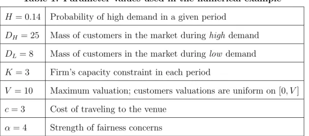
We now present a numerical example to help provide more intuition for the results from the previous section. Table 1 presents the parameter values used for the numerical example.
11The conditions of Proposition 3 are sufficient, but not necessary, for rationing to occur. Lemma
2 shows that Condition 2 ensures setting constant prices is optimal for the entire range of possible values ofv∗ derived in Lemma 1, which may be a stronger condition than necessary for rationing.
Fehr and Schmidt (1999) estimate that participants in their lab experiments have a fairness concern parameter,α, ranging from 0 to 4. We initially perform our numerical analysis for strong fairness concerns, with α= 4. We later repeat our analysis for weaker fairness concerns.12
Table 1. Parameter values used in the numerical example
H = 0.14 Probability of high demand in a given period
DH = 25 Mass of customers in the market during high demand
DL= 8 Mass of customers in the market during low demand
K = 3 Firm’s capacity constraint in each period
V = 10 Maximum valuation; customers valuations are uniform on [0, V]
c= 3 Cost of traveling to the venue
α= 4 Strength of fairness concerns
Given these parameter values, Conditions 1, 2, and 3 hold. Lemma 1 states that the optimal value of v∗ lies in [6.5,8.8]. Lemma 2 states that the firm’s optimal strategy is to set constant prices, and Proposition 3 states that this profit-maximizing price will involve rationing during high demand. We numerically compute that the firm’s optimal price is PL = PH = 4.0, which results in customers traveling to the
venue if their valuation exceeds v∗ = 7.6. During low demand, all purchase attempts succeed; but during high demand, there is rationing and only 49.3% of purchase attempts succeed. The firm sells 1.9 units during low demand and 3.0 units (full capacity) during high demand, and its expected profits in each period are 8.3.
We compare this optimal strategy with two alternative strategies that do not
involve rationing. For constant prices with no rationing, the profit-maximizing price 12As explained by Fehr and Schmidt (1999), a player withα= 4 would be willing to reduce his
own payoff by $1.00 in order to reduce the payoff of another player, who receives a larger payoff, by $1.25, and thus reduce the payoff gap by $0.25.
(for this type of policy) is PL =PH = 5.8, which results in expected profits in each
period of 7.2. For variable prices withno rationing, the profit-maximizing prices (for this type of policy) are PL = 3.0 and PH = 4.1, which results in expected profits in
each period of 6.9.
Table 2. Outcomes for three price strategies
Constant prices Constant prices Variable prices with rationing with no rationing with no rationing Price PH 4.0 5.8 4.1
Price PL 4.0 5.8 3.0
Min. val. to travel v∗ 7.6 8.8 7.5 Fill rate SH 49.3% 100% 100%
Fill rate SL 100% 100% 100%
Quantity QH 3.0 3.0 3.0
Quantity QL 1.9 1.0 2.0
Expected profits E[πt] 8.3 7.2 6.9
Note: Subscripts H and L denote variables for high- and low-demand periods. Table 2 summarizes the outcomes for these three pricing strategies. For this numerical example, the optimal policy with constant prices and rationing during high demand leads to 14.4% higher profits (8.3 vs. 7.2) than the best possible policy with constant prices and no rationing. The optimal policy with constant prices and rationing also leads to 20.6% higher profits (8.3 vs. 6.9) than the best possible policy with variable prices and no rationing.
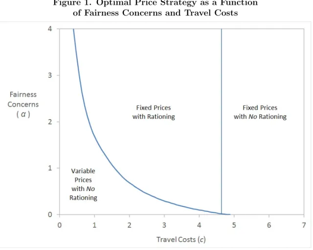
We now repeat our numerical analysis for a larger range of parameter values. Figure 1 presents the optimal price policy for values for the fairness parameter ranging from α = 0 to α = 4, and values of the travel cost parameter ranging from c = 0 to c = 7. The other parameter values used in this figure are the same as for the numerical example presented above.
Figure 1. Optimal Price Strategy as a Function of Fairness Concerns and Travel Costs
As noted in the discussion after Proposition 3, the interaction of fairness concerns with travel costs causes the firm to prefer fixed prices rather than variable prices. Consistent with this intuition, Figure 1 shows that the firm tends to prefer variable pricing when either α or c is sufficiently low, but it prefers fixed pricing when both parameters are large.
Figure 1 also shows that, when c > 4.7, the firm never rations the product. Intuitively, as the sunk cost required to purchase the product increases, the firm serves fewer customers in equilibrium. When this cost is sufficiently high, it is more profitable to set constant prices such that the capacity constraint exactly binds during high demand, so rationing is not required, rather than setting constant prices at a lower level that would require rationing. Thus, rationing can occur for intermediate
3.3
Model Extension: Reputation and Price Policy
This section relaxes the assumption that the firm’s price policy announcement is binding, and we derive conditions in which reputation effects compel the firm not to deviate from its announced policy.
We use the following timing assumptions. The firm first announces a non-binding price policy that specifies PL and PH. As in the previous section, this price policy
announcement affects customers’ utility function, as they derive disutility from paying a price higher than min(PL, PH). Then in each period t:
1. Nature determines the demand state for the period, which the firm observes. 2. The firm decides its price for the period (which can differ from its announced
price policy). Customers do not observe the current demand state or price. 3. Customers who are in the market decide whether to incur the cost to travel to
the venue.
4. Customers who traveled learn the current price, and they have the option to make a purchase attempt. If there is excess demand, then the product is rationed. Payoffs for the period are realized.
A one-shot version of this game, without any price commitment, cannot have an equilibrium with positive profits. Let v∗ denote the minimum valuation of customers who travel in such a potential equilibrium. To maximize profits, the firm would then set its price greater than or equal to the willingness-to-pay of a customer with valuation v∗; however, such a price implies a customer with valuation equal to v∗
did not have an incentive to incur the cost of travel. Therefore, the only possible equilibrium of a one-shot version of this game involves no customers traveling, and the firm setting its price at least as high as V −c, generating zero profits. We focus
on an equilibrium of ourrepeated game in which players revert to the bad equilibrium with zero profits if the firm ever deviates from its announced price policy, which provides the strongest possible incentive for the firm not to deviate.13
A policy of constant prices with rationing during high demand gives the firm a particularly strong incentive to deviate during high-demand periods. The firm can announce such a policy, with constant relatively low prices, to induce customers with fairness concerns to incur the cost of travel. However, once this policy announcement convinces customers to travel, which helps increase sales during low-demand periods, the firm could significantly increase its profits during a high-demand period by raising its price until demand equals capacity. Such a deviation from its announced policy would then cause the game to revert to the bad equilibrium with no profits in future periods. We show that this threat of reduced future profits can sustain a policy of constant prices with rationing during high demand if the following condition holds. The left side of the inequality in this condition is an upper bound on the additional profits a firm can generate by deviating from its price policy (from the equilibrium in Proposition 3) during a high-demand period, and the right side is a lower bound on the expected discounted value of its future profits if it maintains its optimal policy with constant prices.
Condition 4. K v∗−Pb 1+α < 1−δδPb HK+ (1−H)DLV −v∗ V
where price Pb is defined as follows:
b
P ≡v∗− c
1−Hb +HSb H(v∗)
(11) 13For simplicity, we assume, when the period ends, all potential customers learn about any
deviation from the firm’s price policy. For example, customers might learn about deviations through news stories or word of mouth. If only customers who traveled in the current period observed deviations, then our conditions for sustaining a fixed price policy would need to be modified, but results similar in spirit would still hold.
As we would expect based on folk theorem results, this condition holds if the discount factorδis sufficiently close to one. However, for anyδ >0, this condition also holds if customers have sufficiently strong fairness concerns, that is, ifαis sufficiently high. Fairness concerns reduce the firm’s temptation to deviate from its announced price policy because customers with strong fairness concerns are not willing to pay a large premium over the firm’s announced prices, even after they have incurred the cost of travel. As shown in the section 3.1, strong fairness concerns along with positive travel costs imply that the firm’s profit maximizing policy is to set constant prices; furthermore, the results in the current section show that fairness concerns also help the firm sustain such a policy of constant prices by reducing its incentive to deviate from this policy in a repeated game.
Proposition 4. If the conditions for rationing in Proposition 3 hold, and the firm is patient enough or customers have strong enough fairness concerns that Condition 4 holds, then the firm can sustain its profit-maximizing policy of constant prices with rationing during high demand, even if its price policy announcement is not binding.
For the numerical example in section 3.2, Condition 4 holds for anyα ≥1,c≤4, and δ ≥ 0.68. If this condition holds, the firm can sustain its optimal price policy, based on the threat of loss of reputation and lost future profits if it ever deviates from this policy.
3.4
Model Extension: Separate Search and Travel Costs
This section shows that our key findings still hold if search and travel decisions occur sequentially, so customers can search before deciding whether to travel to the venue, or they can travel directly to the venue without searching. We denote search costs by c1 and travel costs by c2, where 0 ≤c1 ≤ Hcb 2. The latter condition ensures that a customer who, in equilibrium, makes purchase attempts only during low demand
prefers to search before traveling to avoid the expected cost of traveling during high demand.
The timing for this model extension is as follows. The firm first announces a price policy that specifies PL and PH, and in each periodt:
1. Nature determines the demand state and the set of customers who are available in the market. The firm automatically sets its price according to its announced policy for the given demand state.14 Customers do not observe the current demand state or price.
2. Customers who are in the market decide whether to incur the search cost c1 to learn the price for the current period.
3. Customers who are in the market decide whether to incur the cost c2 to travel to the location where the product is sold. Customers who incur this travel cost learn the price even if they did not previously search.
4. Customers who traveled to the product location have the option to make a purchase attempt. If there is excess demand, then the product is rationed. Payoffs for the period are realized.
Under these timing assumptions, during periods with excess demand, customers must travel to the venue to learn whether they are able to purchase and consume the product in the current period. For example, customers who purchase electronic tickets to Disneyland sometimes find they unable to enter the park on a given day, in which case they must wait and use their tickets on a different day.15 In principle, we could derive similar results using alternative timing assumptions, in which customers who 14In this section, we assume the price policy announcement is binding, but in principle we could
allow for endogenous price commitment as in the previous section.
search online learn immediately whether they are able to consume the product on their preferred day.16
If the firm sets fixed prices (PH =PL), then searching for the current price provides
no information. In this case, customers follow the same strategy as in section 3.1. There is no search, and each customer travels to the venue if the expected value of doing so exceeds the cost of travel.17
On the other hand, if the firm uses a variable price policy (PH 6= PL), there are
three possible strategies a customer with valuation vi could follow. For a customer
who does not make purchase attempts during any demand state, there is no reason to search or travel, and this strategy results in zero utility.
Given the condition c1 ≤Hcb 2, for a customer who makes purchase attempts only during low demand, it is optimal to search first to avoid the expected cost of traveling during high demand, and this strategy results in the following expected utility:
(1−Hb)
SL(vi−PL)−c2
−c1 (12)
The customer prefers this strategy over the strategy of never purchasing if his valuation vi is high enough that the above expression is positive.
Finally, for a customer who makes purchase attempts during both demand states, it is optimal to travel directly to the venue without searching, as searching would impose additional costs without affecting his travel decision. A necessary condition for 16Under this alternative assumption, rationing could occur at the search stage as customers who
search learn whether they can purchase in the current period, or rationing could occur at the the venue itself as customers with high valuations would travel directly to the venue without searching if the success probability were sufficiently high.
17If we assumed customers who search could observe both the priceand the demand state, then in
some cases, customers might want to search even with a policy of constant prices, in order to avoid travel during high-demand periods with rationing. However, this alternative assumption allowing customers who search to learn the demand state would not affect our results. All customers who travel in the fixed-price equilibrium derived in this section gain greater expected utility from traveling directly to the venue than they would from searching and traveling only when demand is low.
this strategy to be optimal is the customer’s valuation must exceed the price during both demand states, which implies this strategy results in the following expected utility:18 b HSH vi−PH −α(PH −PL) + (1−Hb)SL(vi−PL)−c2 (13)
By comparing (13) with (12), we find that a customer would prefer to travel directly to the venue and purchase during both demand states rather than searching and purchasing only during low demand if his valuation is high enough that the following expression is positive:
b
HSH(vi−PH −α(PH −PL))−c2
+c1 (14) Based on the preceding analysis, for any given prices and success probabilities, we can compute cutoff values v∗1 and v∗2, where c2 ≤ v1∗ ≤ v2∗ ≤V, such that customers with valuations less thanv∗1 never purchase, those with valuations betweenv∗1 and v2∗
search and travel to the venue only during low demand, and those with valuations greater than v∗2 travel directly to the venue and always make purchase attempts. Because the low-demand success probability SL is a weakly increasing continuous
function of v1∗, and the high-demand success probability SH is a weakly increasing
continuous function of v∗2, for any given price policy, we can compute values of v1∗
and v2∗ such that customers’ search and travel behavior are optimal given the prices and success probabilities. In some cases, v1∗ =v∗2. For example, if prices and success probabilities for purchase attempts have sufficiently little variation across demand states, then a customer would either never purchase or always travel directly to the
18As in the previous sections, these derivations focus on policies for whichP
L≤PH, which is true
venue, and no customers would search.19
Similar to the analysis of the main version of the model in section 3.1, for this model extension we now derive sufficient conditions for rationing to occur in equilibrium. The first condition is that capacity satisfies:
Condition 5. DL(V−c2)
2V < K <
DH(V−c2) 2V
We show the above condition ensures, in equilibrium, the minimum valuation of customers who purchase during low demand, v1∗, lies in the interval [v∗1, v∗1], defined as follows: v∗1 = V +c2 2 (15) v∗1 =V 1− K DH (16) We next show that constant prices generate greater profits than variable profits for any value ofv∗1 in the interval specified above, ifc1 is sufficiently close toHcb 2 and the following condition also holds.
Condition 6. v∗1 −v∗1 < αc2 1−Hb
Finally, given constant prices, we show the firm serves customers with valuations strictly below v∗1 during both demand states, which requires rationing during high demand, if the following condition holds.
Condition 7. V1− 2K DH > c2 1−Hb +(1−HKVH)D L
Therefore, if all of these conditions hold, the firm sets constant prices with rationing during high demand.
19Formally, by deriving the minimum values ofv
i that make (12) and (14) positive, we find there
is a segment of customers who search only if PL+ [c1/(1−Hb) +c2)]/SL < PH+α(PH−PL) +
[−c1/Hb+c2)]/SH, in which case there is a range of valuations for which (12) is positive but (14) is
Proposition 5. In the model extension with separate search and travel costs, if Conditions 5, 6, and 7 hold, and c1 is sufficiently close to Hcb 2, there is a unique equilibrium in which the firm sets the same price during high and low demand (PH =PL), with rationing during high demand.
For notational simplicity, we have stated this proposition for the case in which
c1 →Hcb 2. The proof of Proposition 5 in the appendix derives more general conditions
for rationing. If c1 < Hcb 2 and we do not impose c1 → Hcb 2, then in place of
Condition 6, we require that the profits from fixed prices in equation (41) are greater than the profits from variable prices in equation (39) in the appendix.20 On the other hand, ifc1 >Hcb 2, then customers never search, and this model extension is equivalent to the main version of the model in section 3.1.
The intuition for Proposition 5 is similar to the intuition for Proposition 3. If fairness concerns are strong enough, and search costs and travel costs are both large enough, then the firm maintains low prices with rationing during high demand to encourage customers to travel to the venue duringlow demand. The main difference is Proposition 5 requires that search costs (c1) cannot be too low relative to a customer in the market’s perceived probability of high demand based on rational Bayesian updating (Hb) times travel costs (c2). Intuitively, if search costs are much lower than travel costs, then setting constant prices to encourage people to travel directly to the venue is not an efficient way to increase purchases during low demand. In such cases, it would be more profitable to use variable pricing and allow customers to search to discover the demand state.
20For a given value ofv∗
1, a reduction in search costs (c1) has three effects on the profits from a
variable price policy. First, reduced search costs allow the firm to increasePL while still attracting
the same customers during low demand. Second, given fairness concerns, the resulting increase in
PLimplies, all else equal, the firm can increasePH while still providing the same amount of utility to
customers during high demand. However, the third effect, which tends to offset the second, is that reduced search costs imply the firm must provide greater utility to customers during high demand to induce them to travel to the venue and purchase during both periods rather than searching and purchasing only during low demand. The conditions for rationing must account for all three effects when comparing the profits from variable versus fixed price policies.
As was the case for Proposition 3, the conditions of Proposition 5 are sufficient but not necessary for rationing to occur in equilibrium. In fact, we show that strictly positive fairness concerns, search costs, and travel costs are all necessary conditions for rationing.
Proposition 6. In the model extension with separate search and travel costs, if
customers do not have fairness concerns (α= 0), there is no rationing in equilibrium.
Proposition 7. In the model extension with separate search and travel costs, if either search costs are zero (c1 = 0) or travel costs are zero (c2 = 0), there is no rationing in equilibrium.
The intuition for these results is similar to the intuition for Propositions 1 and 2. If customers do not have fairness concerns, then setting PH low enough to generate
shortages is not an efficient way to induce customers to travel to the venue; and if search costs or travel costs are zero, then the firm can raise PH until no rationing is
necessary during high-demand periods without affecting its profits during low-demand periods.
Finally, we show that, if the firm can reduce search costs, making it easier for customers to find current price information, then doing so increases equilibrium profits.21
Proposition 8. In the model extension with separate search and travel costs, a
reduction in search costs (c1) weakly increases the firm’s equilibrium profits.
Intuitively, low search costs make it easy for customers with low valuations to avoid travel when prices are high. Therefore, a reduction in search costs allows the firm to use variable pricing, with price increases during peak demand, without causing a significant reduction in sales during low-demand periods.
21In the parameter range for which the firm sets variable prices, a marginal reduction in search
costs leads to strictly higher profits. In the parameter range for which the firm setsfixed prices, a marginal reduction in search costs has no effect on profits.
4
Conclusion
This paper studies an important problem in markets where a firm has a capacity constraint and customers have fairness concerns. We show the firm may want to set constant prices to avoid imposing disutility from unfairness on customers, who would have to incur travel costs to learn the current price under a variable price policy. However, if the firm can communicate each period’s price to customers before they incur travel costs, so that customers have the option not to travel during high demand, then the firm does use variable pricing.
Kahneman et al. (1986) claim that price variation based on demand fluctuations antagonizes customers, which can cause firms to set stable prices and experience shortages during peak demand. We predict that fairness concerns cause shortages only if customers face uncertainty about each period’s demand level, which the firm cannot resolve, either because the firm itself faces fundamental uncertainty in forecasting demand, or because it does not have a low-cost way of communicating these forecasts to its customers.
Future research could extend our model to explore other ways firms can manage demand spikes. For example, an exogenous capacity constraint, as in our model, is a reasonably accurate assumption for many entertainment firms. Disneyland has limited room to expand because of its location in the city of Anaheim (Vaux 2010). Similarly, the Boston Red Sox baseball team cannot, from a structural engineering perspective, add many new seats to their current stadium; they would need to build an entirely new stadium to increase their seating capacity (Charlotin 2010). However, some firms can expand capacity quickly. When ridesharing services such as Uber and Lyft increase prices during peak demand, it encourages more drivers to become active during peak demand (Kosoff 2015). Future research could incorporate endogenous capacity into our model to allow for this additional benefit of increased prices.
Future research could also explore different rationing rules. For example, a firm could potentially use observable customer characteristics, such as location of resi-dence, to decide which customers are able to purchase during high-demand periods. Such customers will have greater willingness to incur the cost of travel if they are confident their purchase attempts will be successful.
References
Anderson, E. T. and D. I. Simester (2010). Price stickiness and customer antagonism.
The Quarterly Journal of Economics 125(2), 729–765.
Becker, G. S. (1991). A note on restaurant pricing and other examples of social influences on price. Journal of Political Economy 99(5), 1109–1116.
Bolton, L. E., L. Warlop, and J. W. Alba (2003). Consumer perceptions of price (un)fairness. Journal of Consumer Research 29(4), 474–491.
Camerer, C. F. and R. H. Thaler (1995). Anomalies: Ultimatums, dictators and manners. Journal of Economic Perspectives 9(2), 209–219.
Charlotin, R. (2010). Boston Red Sox need a new Fenway Park. Bleacher Report. Chen, Y., O. Koenigsberg, and Z. J. Zhang (2017). Pay-as-you-wish pricing.
Market-ing Science 36(5), 780–791.
Cui, T. H., J. S. Raju, and Z. J. Zhang (2007). Fairness and channel coordination.
Management Science 53(8), 1303–1314.
Drayer, J., S. L. Shapiro, and S. Lee (2012). Dynamic ticket pricing in sport: An agenda for research and practice. Sport Marketing Quarterly 21(3), 184–194. Economist (2016). Disney discovers peak pricing. https://www.economist.com/
blogs/freeexchange/2016/02/price-discrimination-land.
Englmaier, F., L. Gratz, and M. Reisinger (2012). Price discrimination and fairness concerns. Working paper.
Feeney, M. (2014). The economics of Uber’s surge pricing. Cato Institute. https: //www.cato.org/blog/economics-uber-surge-pricing.
Fehr, E. and K. M. Schmidt (1999). A theory of fairness, competition, and coopera-tion. The Quarterly Journal of Economics 114(3), 817–868.
Fritz, B. (2016). Disney rolls out seasonal pricing for one-day park tickets. Wall Street Journal.
Gilbert, R. J. and P. Klemperer (2000). An equilibrium theory of rationing. The RAND Journal of Economics 31(1), 1–21.
Guo, L. (2015). Inequity aversion and fair selling. Journal of Marketing Re-search 52(1), 77–89.
Guo, X. and B. Jiang (2016). Signaling through price and quality to consumers with fairness concerns. Journal of Marketing Research 53(6), 988–1000.
Haydu, S. (2016). New Year’s Eve ride guide. Uber Newsroom.
Hoffman, E., K. McCabe, K. Shachat, and V. Smith (1994). Preferences, property rights, and anonymity in bargaining games. Games and Economic Behavior 7(3), 346 – 380.
Kahneman, D., J. L. Knetsch, and R. Thaler (1986). Fairness as a constraint on profit seeking: Entitlements in the market. The American Economic Review 76(4), 728– 741.
Kosoff, M. (2015). Don’t complain about Uber’s surge pricing tonight. Business Insider.
Lefton, T. and J. Lombardo (2003). Stern’s NBA shows its transition game. Street and Smith’s Sports Business Journal.
Leonhardt, D. (2005). Why variable pricing fails at the vending machine. New York Times.
Levy, D., M. Bergen, S. Dutta, and R. Venable (1997). The magnitude of menu costs: Direct evidence from large U.S. supermarket chains. The Quarterly Journal of Economics 112(3), 791–824.
Li, K. J. and S. Jain (2016). Behavior-based pricing: An analysis of the impact of peer-induced fairness. Management Science 62(9), 2705–2721.
Liu, Q. and S. Shum (2013). Pricing and capacity rationing with customer disap-pointment aversion. Production and Operations Management 22(5), 1269–1286. Martin, H. (2014). Disney parks on both coasts close temporarily on Christmas. Los
Angeles Times.
Mohammed, R. (2015). Of course disney should use surge pricing at its theme parks.
Harvard Business Review.
Nasiry, J. and I. Popescu (2012). Advance selling when consumers regret.Management Science 58(6), 1160–1177.
Okada, T. (2014). Third-degree price discrimination with fairness-concerned con-sumers. The Manchester School 82(6), 701–715.
Ozer, O. and Y. Zheng (2016). Markdown or everyday low price? The role of behavioral motives. Management Science 62(2), 326–346.
Rogers, J. (2016). LA tries to cope with rain in a place where rain is rare. Associated Press. https://www.businessinsider.com/ ap-la-tries-to-cope-with-rain-in-a-place-where-rain-is-rare-2016-1.
Rotemberg, J. J. (2005). Customer anger at price increases, changes in the frequency of price adjustment and monetary policy. Journal of Monetary Economics 52(4), 829 – 852. {SNB}.
Rovell, D. (2001). Jordan is just the ticket to boost NBA attendance. Espn.com.
http://assets.espn.go.com/nba/s/2001/0925/1255329.html.
Shapiro, S. L., J. Drayer, and B. Dwyer (2016). Examining consumer perceptions of demand-based ticket pricing in sport. Sport Marketing Quarterly 25(1), 34–46. Su, X. (2010). Optimal pricing with speculators and strategic consumers.
Manage-ment Science 56(1), 25–40.
Thaler, R. (1985). Mental accounting and consumer choice. Marketing Science 4(3), 199–214.
Vaux, R. (2010). Disney World compared to Disneyland. USA Today Travel Tips. Weiner, J. (2014). Is Uber’s surge pricing fair? Washington Post.
https://www.washingtonpost.com/blogs/she-the-people/wp/2014/12/ 22/is-ubers-surge-pricing-fair.
Wernerfelt, B. (1994). Selling formats for search goods. Marketing Science 13(3), 298–309.
Appendix: Proofs
Proof of Proposition 1 For any price policy that leads to rationing, we will show
that, if α = 0, there is a profitable deviation, which implies that such a price policy cannot be optimal.
Suppose rationing occurs only during high demand. If PH < v∗ < PL, then the
marginal customer with valuation v∗ buys only during high demand. In this case, a small increase inPH increases high-demand profits (PHK), without causing any sales
reduction during low demand, despite the resulting marginal increase inv∗. Similarly, if PL< v∗ ≤PH, then the marginal customer with valuationv∗ buys only during low
causing any sales reduction during low demand, because this price change does not affect v∗. In both cases, a small increase inPH leads to greater total profits.
The only way a marginal increase in PH can reduce sales during low demand is if
PH < v∗ and PL ≤v∗, in which case such a price increase leads to a higher value of
v∗ and reduces low-demand sales. Whenv∗ is weakly greater than the price for both demand states, prices must satisfy equation (5) as follows:
b
HSH(v∗)(v∗−PH) + (1−Hb)(v∗−PL) =c (17)
Suppose the firm increasesPH by=v∗−PH. In order to induce customers with the
same v∗ to continue traveling, it must decrease PL by
b
HSH(v∗) 1−Hb
so that (17) continues to hold. The net effect on expected profits of these price changes is:
HK + HSb H(v ∗) 1−Hb (1−H)DL V −v∗ V (18) Inserting Hb = HD HDH H+(1−H)DL, (1−Hb) = (1−H)DL HDH+(1−H)DL, and SH(v ∗) = KV DH(V−v∗) into this expression, we find that the net effect on expected profits is zero. Because we increased PH by, where =v∗−PH, we now havePL< v∗ =PH. As shown above,
further increases in PH increase profits during high demand without affecting sales
during low demand. Therefore, the initial price policy with rationing only during high demand could not be optimal.
Similar analysis shows that a price policy with rationing only during low demand cannot be optimal. Finally, if rationing occurs during both demand states, then the firm always sells K units, and a small price increase leads to greater profits. Thus, if
Proof of Proposition 2 Ifc= 0, then all customers always travel. Suppose a price policy leads to rationing during high demand. Increasing PH leads to greater profits
during high demand without affecting travel behavior. If PH ≥ PL, this increase
in PH does not affect sales during low demand. On the other hand, if PH < PL
this increase in PH leads to weakly greater sales during low demand by reducing the
effect of fairness concerns on low-demand sales. In either case, total expected profits increase. Therefore, rationing during high demand cannot be optimal. A similar argument shows that rationing during low demand cannot be optimal. QED
Proof of Lemma 1 We first show that any price strategy that leads to a minimum
travel valuation of v∗ > v∗ cannot be the firm’s profit-maximizing strategy. The upper bound v∗ was defined such that the firm always has excess capacity ifv∗ > v∗, so all purchase attempts succeed, and the equation (5) becomes:
b
Hmax[v∗−PH −α(PH −PL),0] + (1−Hb) max[v∗−PL,0] = c (19)
We will show that, for any v∗ > v∗, the most profitable way to induce customers with valuation v∗ to travel is by setting constant prices, PL =PH =v∗−c. Suppose
the firm starts with these constant prices. Now suppose the firm increases PH by
a small amount . If customers have no fairness concerns, so α = 0, then in order for customers with the same valuation v∗ to continue traveling, the firm must reduce
PL by (1−Hb
b
H) so that equation (19) continues to hold. Therefore, the net effect on expected profits of these price changes is HDHV−v
∗ V − b H (1−Hb) (1−H)DLV−v ∗ V . Note that Hb (1−Hb) = HDH
(1−H)DL. Therefore, forα = 0 and a given value of v
∗, the net effect on
expected profits of this deviation from constant prices isHDHV−v ∗
V [−] = 0, so the
firm is indifferent between constant prices and small deviations from constant prices. On the other hand, if α > 0, increasing PH by requires the firm to make an even
larger reduction in PL in order for (19) to continue to hold for the same v∗, so that
the net effect on expected profits is strictly negative. Similar derivation show that, starting with constant prices and a given value of v∗, the firm would not want to increasePL and reduce PH to induce the same value of v∗.
We also need to check non-local deviations. If the firm sets PH high enough that
PH +α(PH −PL)> v∗, then customers with valuation v∗ no longer purchase during
high demand, even if PL decreases enough that these customers continue to travel
and purchase during low demand. The firm’s profits during each high demand period become DHPH[V−PH−α(PH−PL)]
V . Taking the first derivative of these profits with respect
to PH, we have DH[V
−2PH−α(2PH−PL)]
V . Under Condition 1, this derivative is negative
for PH > v∗, so the firm could increase its profits by reducing its price. Therefore,
this non-local deviation from constant prices is not optimal. Similar analysis shows that a large (non-local) increase PL cannot be optimal, and therefore constant prices
are the profit-maximizing way to induce customer travel for any v∗ > v∗. With constant prices, the firm’s expected profits as a function of v∗ are:
E[πt] = [HDH + (1−H)DL](v∗−c) V −v∗ V (20)
Taking the first derivative, we have:
dE[πt] dv∗ = [HDH + (1−H)DL] V +c−2v∗ V (21)
Condition 1 guarantees v∗ > V2+c. Therefore, this derivative is negative for any
v∗ > v∗, and prices that lead to any suchv∗ cannot be optimal because the firm could increase its profits by reducing its prices.
We next show that any price strategy that leads to a minimum travel valuation of
that the firm could increase its profits by raising prices during one or both demand states. We need to consider three cases.
First, suppose the firm sets a price policy with PL < PH, and v∗ is such that
PL < v∗ < PH + α(PH −PL). In this case, customers with valuation v∗ makes
purchase attempts only during low demand periods. If the firm has excess demand even during low-demand periods, then profits during low demand are PLK. In this
case, a small increase inPL leads to greater profits during low demand. On the other
hand, if the firm can satisfy all customers during low demand, then its profits during low demand are PLDLV−v
∗
V , where pricePL must satisfy equation (5):
(1−Hb)(v∗−PL) =c (22)
Solving for price, we have PL = v∗− 1−c
b
H, which implies profits during low demand
periods are: πL = v∗− c 1−Hb DL V −v∗ V (23)
Taking the first derivative, we have:
dπL dv∗ =DL V + c 1−Hb −2v∗ V (24)
This derivative is positive for all v∗ < v∗. Therefore, increasing PL would increase
profits during low demand, and would also weakly increase profits during high demand by reducing the effect of fairness concerns on high-demand profits.
Next, suppose the firm sets a price policy with PH < PL, and v∗ is such that
PH < v∗ < PL+α(PL−PH). Given v∗ < v∗, the firm has excess demand during high
demand periods, during which it generates profits PHK. A similar argument to the
Finally, suppose the firm sets a price policy such thatPL< v∗andPH < v∗, so that
customers with valuationv∗ purchase during both demand states. A similar argument to the one described above (for v∗ > v∗) shows that constant prices (PH = PL)
are the optimal way to induce such an outcome. In particular, for α = 0 and a given value of v∗, if the firm starts with constant prices and increases PH by , it
must decrease PL by
b
HSH(v∗) 1−Hb
to induce customers with the same v∗ to continue traveling. This deviation leads to zero effect on expected profits (see the proof of Proposition 1 for additional detail). However, if α > 0, the firm must make an even larger reduction inPLto maintain the samev∗, which leads to strictly lower expected
profits. Therefore, constant prices are optimal for any policy in which customers with valuation v∗ purchase during both demand states.
Given PH = PL = P and v∗ < v∗, if the firm has excess demand during both
demand states, then a small price increase leads to greater profits. On the other hand, if the firm has excess demand during high demand periods but not during low demand, then prices must satisfy (5) as follows:
b
HSH(v∗)(v∗−P) + (1−Hb)(v
∗−
P) = c (25) Solving for price, we have P =v∗− c
1−Hb+HSb H(v∗), which implies expected profits are:
E[πt] = v∗− c 1−Hb +HSb H(v∗) HK+ (1−H)DL V −v∗ V (26) Inserting (1−Hb) = (1 −H)DL (1−H)DL+HDH, Hb = HDH (1−H)DL+HDH, and SH(v ∗) = KV DH(V−v∗) into the above equation, we have:
E[πt] =v∗ HK+ (1−H)DL V −v∗ V −c V −v∗ V [(1−H)DL+HDH] (27)