IHS Economics Series
Working Paper 249
February 2010
Risk Shocks and Housing Markets
Victor Dorofeenko
Gabriel S. Lee
Kevin D. Salyer
Impressum Author(s):
Victor Dorofeenko, Gabriel S. Lee, Kevin D. Salyer
Title:
Risk Shocks and Housing Markets
ISSN: Unspecified
2010 Institut für Höhere Studien - Institute for Advanced Studies (IHS)
Josefstädter Straße 39, A-1080 Wien
E-Mail: o [email protected]ffi
Web: www .ihs.ac. a t
All IHS Working Papers are available online: http://irihs. ihs. ac.at/view/ihs_series/
Risk Shocks and Housing
Markets
Victor Dorofeenko, Gabriel S. Lee, Kevin D. Salyer
249
Reihe Ökonomie
Economics Series
249
Reihe Ökonomie
Economics Series
Risk Shocks and Housing
Markets
Victor Dorofeenko, Gabriel S. Lee, Kevin D. Salyer
February 2010
Institut für Höhere Studien (IHS), Wien
Institute for Advanced Studies, Vienna
Contact: Victor Dorofeenko
Department of Economics and Finance Institute for Advanced Studies Stumpergasse 56 1060 Vienna, Austria : +43/1/599 91-183 email: [email protected] Gabriel S. Lee IREBS University of Regensburg Universitätsstraße 31 93053 Regensburg, Germany : ++49/941/943.5060 email: [email protected] and
Institute for Advanced Studies
Kevin D. Salyer (Corresponding Author) Department of Economics
University of California Davis, CA 95616, USA email: [email protected]
Founded in 1963 by two prominent Austrians living in exile – the sociologist Paul F. Lazarsfeld and the economist Oskar Morgenstern – with the financial support from the Ford Foundation, the Austrian Federal Ministry of Education and the City of Vienna, the Institute for Advanced Studies (IHS) is the first institution for postgraduate education and research in economics and the social sciences in
Austria. The Economics Series presents research done at the Department of Economics and Finance
and aims to share “work in progress” in a timely way before formal publication. As usual, authors bear full responsibility for the content of their contributions.
Das Institut für Höhere Studien (IHS) wurde im Jahr 1963 von zwei prominenten Exilösterreichern – dem Soziologen Paul F. Lazarsfeld und dem Ökonomen Oskar Morgenstern – mit Hilfe der Ford-Stiftung, des Österreichischen Bundesministeriums für Unterricht und der Stadt Wien gegründet und ist somit die erste nachuniversitäre Lehr- und Forschungsstätte für die Sozial- und
Wirtschafts-wissenschaften in Österreich. Die Reihe Ökonomie bietet Einblick in die Forschungsarbeit der
Abteilung für Ökonomie und Finanzwirtschaft und verfolgt das Ziel, abteilungsinterne Diskussionsbeiträge einer breiteren fachinternen Öffentlichkeit zugänglich zu machen. Die inhaltliche Verantwortung für die veröffentlichten Beiträge liegt bei den Autoren und Autorinnen.
Abstract
This paper analyzes the role of uncertainty in a multi-sector housing model with financial frictions. We include time varying uncertainty (i.e. risk shocks) in the technology shocks that affect housing production. The analysis demonstrates that risk shocks to the housing production sector are a quantitatively important impulse mechanism for the business cycle. Also, we demonstrate that bankruptcy costs act as an endogenous markup factor in housing prices; as a consequence, the volatility of housing prices is greater than that of output, as observed in the data. The model can also account for the observed countercyclical behavior of risk premia on loans to the housing sector.
Keywords
Agency costs, credit channel, time-varying uncertainty, residential investment, housing production, calibration
JEL Classification
E4, E5, E2, R2, R3Comments
We wish to thank David DeJong, Aleks Berenten, and Alejandro Badel for useful comments and suggestions. We also benefitted from comments received during presentations at: the Humboldt University, University of Basel, European Business School, Latin American Econometric Society Meeting 2009, and AREUEA 2010. We are especially indebted to participants in the UC Davis and IHS Macroeconomics Seminar for insightful suggestions that improved the exposition of the paper. We also gratefully acknowledge financial support from Jubiläumsfonds der Oesterreichischen Nationalbank (Jubiläumsfondsprojekt No. 13040).
Contents
1 Introduction
1
2 Model
Description
3
2.1 Production ... 3 2.1.1 Firms ... 3 2.1.2 Households ... 72.2 The Credit Channel ... 9
2.2.1 Housing Entrepreneurial Contract ... 9
2.2.2 Housing Entrepreneurial Consumption and House Prices ... 14
2.2.3 Financial Intermediaries ... 16
3 Equilibrium
16
4 Calibration
and
Data
20
5 Results
24
5.1 Steady State Values, Second Moments and Lead - Lag Patterns ... 245.2 Dynamics: Impulse Response Functions ... 27
5.3 Some Final Remarks ... 29
References 3
6 Data
Appendix
3
1
Introduction
The Great Recession of 2009 has dramatically underscored the importance that …nancial and housing markets have for the behavior of the macroeconomy. To better understand the role that these markets play in aggregate ‡uctuations, this paper presents a calibrated general equilibrium model that incorporates these factors but also introduces an impulse mechanism, time varying uncertainty, that, until recently, has not received much attention in the literature.1 In particular, we analyze the role of time varying uncertainty (i.e. risk shocks) in a multi-sector real business cycle model that includes housing production (developed by Davis and Heathcote, (2005)) and a …nancial sector with lending under asymmetric information (e.g. Carlstrom and Fuerst, (1997), (1998); Dorofeenko, Lee, and Salyer, (2008)). We model risk shocks as a mean preserving spread in the distribution of the technology shocks a¤ecting house production and explore how changes in uncertainty a¤ect equilibrium characteristics.2
Our aim in examining this environment is twofold. First, we want to develop a framework that can capture one of the main components of the current …nancial crises, namely, changes in the risk associated with the housing sector. In our analysis, we focus entirely on the variations in risk associated with the production of housing and the consequences that this has for lending and economic activity. Hence our analysis is very much a fundamental-based approach so that we side step the delicate issue of modeling housing bubbles and departures from rational expectations. The results, as discussed below, suggest (to us) that this conservative approach is warranted.3 Second, we want to cast the analysis of risk shocks in a model that is broadly consistent with some of
1 Some recent papers that have examined the e¤ects of uncertainty in a DSGE framework include Bloom et al. (2008), Fernandez-Villaverde et al. (2009), and Christiano et al. (2008). The last paper is most closely related to the analysis presented here in that it also uses a credit channel model.
2 Some of the recent works which also examine housing and credit are: Iacoviello and Minetti (2008) and Iacoviello and Neri (2008) in which a new-Keynesian DGSE two sector model is used in their empirical analysis; Iacoviello (2005) analyzes the role that real estate collateral has for monetary policy; and Aoki, Proudman and Vliegh (2004) analyse house price ampli…cation e¤ects in consumption and housing investment over the business cycle. None of these analyses use risk shocks as an impulse mechanism.
3 In a closely related analysis, Kahn (2008) also uses a variant of the Davis and Heathcote (2005) framework in order to analyze time variation in the growth rate of productivity in a key sector (consumption goods). He demonstrates that a change in regime growth, combined with a learning mechanism, can account for some of the observed movements in housing prices.
the important stylized facts of the housing sector such as: (i) residential investment is about twice as volatile as non-residential investment and (ii) residential investment and non-residential investment are highly procyclical.4
To that end, we employ the Davis and Heathcote (2005) housing model which, as demonstrated by the authors, can replicate the high volatility observed in residential investment despite the absence of any frictions in the economy. The recent analysis in Christiano et al. (2008), however, provides compelling evidence that …nancial frictions play an important role in business cycles and, given the recent …nancial events, it seems reasonable to investigate this role when combined with a housing sector.5 Consequently, we modify the Davis and Heathcote (2005) analysis by adding a …nancial sector in the economy and require that housing producers must …nance their inputs via loans from the banking sector. This modi…cation appears to be important; for instance, we show that by incorporating an explicit …nancial market into this model, we can produce large movements in housing prices, a feature of the data that was missing in the Davis and Heathcote (2005) analysis. We also demonstrate that housing prices in our model are a¤ected by expected bankruptcies and the associated agency costs; these serve as an endogenous, time-varying markup factor a¤ecting the price of housing. The volatility in this markup translates into increased volatility in housing prices. Moreover, the model implies that this endogenous markup to housing as well as the risk premium associated with loans to the housing sector should be countercyclical; both of these features are seen in the data.6
Our analysis …nds that plausible calibrations of the model with time varying uncertainty pro-duce a quantitatively meaningful role for uncertainty over the housing and business cycles. For
4 One other often mentioned stylized fact is that housing prices are persistent and mean reverting (e.g. Glaser and Gyourko (2006)). See Figure 1 and Table 4 for these cyclical and statistical features during the period of 1975 until the second quarter of 2007.
5 Christiano et al. (2008) use a New Keynesian model to analyze the relative importance of shocks arising in the labor and goods markets, monetary policy, and …nancial sector. They …nd that time-varying second moments, i.e. risk shocks, are quantitatively important relative to the the other impulse mechanisms.
6 In addition to these cyclical features, a marked feature of the housing sector has been the growth in residential and commercial real estate lending over the last decade. As shown in Figure 2, residential real estate loans (excluding revolving home equity loans) account for approximately50%of total lending by domestically chartered commercial banks in the United States over the period October 1996 to July 2007. Figure 3 shows the strong co-movement between the amount of real estate loans and house prices.
instance, we compare the impulse response functions for aggregate variables (such as output, consumption expenditure, and investment) due to a 1% increase in technology shocks to the con-struction sector to a 1% increase in uncertainty to shocks a¤ecting housing production. We …nd that, quantitatively, the impact of risk shocks is almost as great as that from technology shocks. This comparison carries over to housing market variables such as the price of housing, the risk premium on loans, and the bankruptcy rate of housing producers. The model is not wholly sat-isfactory in that it can not account for the lead-lag structure of residential and non-residential investment but this is not surprising given that the analysis focuses entirely on the supply of housing. Still, we think the approach presented here provides a useful start in studying the e¤ects of time-varying uncertainty on housing, housing …nance and business cycles.
2
Model Description
As stated above, our model builds on two separate strands of literature: Davis and Heathcote’s (2005) multi-sector growth model with housing, and Dorofeenko, Lee and Salyer’s (2008) credit channel model with time-varying uncertainty. For expositional clarity, we …rst brie‡y outline our variant of the Davis and Heathcote model and then introduce the credit channel model.
2.1
Production
2.1.1 Firms
The economy consists of two agents, a consumer and an entrepreneur, and four sectors: an in-termediate goods sector, a …nal goods sector, a housing goods sector and a banking sector. The intermediate sector is comprised of three perfectly competitive industries: a building/construction sector, a manufacturing sector and a service sector. The output from these sectors are then com-bined to produce a residential investment good and a consumption good which can be consumed or used as capital investment; these sectors are also perfectly competitive. Entrepreneurs
com-bine residential investment with a …xed factor (land) to produce housing; this sector is where the lending channel and …nancial intermediation play a role.
Turning …rst to the intermediate goods sector, the representative …rm in each sector is char-acterized by the following Cobb-Douglas production function:
xit=kiti(nitexpzit)1 i (1)
wherei=b; m; s(building/construction, manufacture, service),kit; nit;andzit are capital,
house-hold labor, and a labor augmenting productivity shock respectively for each sector, with i being
the share of capital for sector i.7 In our calibration we set
b < m re‡ecting the fact that
the manufacturing sector is more capital intensive (or less labor intensive) than the construction sector.
Productivity in each sector exhibits stochastic growth as given by:
zi=tgz;i+ ~zi (2)
where gz;iis the trend growth rate in sector i.
The vector of technology shocks,~z= (~zb;z~m;z~s), follows anAR(1) process:
~zt+1=B ~zt+~"t+1 (3)
The innovation vector~"is distributed normally with a given covariance matrix ".8
These intermediate …rms maximize a conventional static pro…t function every period. That is,
7 Real estate developers, i.e. entrepreneurs, also provide labor to the intermediate goods sectors. This is a technical consideration so that the net worth of entrepreneurs, including those that go bankrupt, is positive. Labor’s share for entrepreneurs is set to a trivial number and has no e¤ect on output dynamics. Hence, for expositional purposes, we ignore this factor in the presentation.
8 In their analysis, Davis and Heathcote (2005) introduced a government sector characterized by non-stochastic tax rates and government expenditures and a balanced budget in every period. We abstract from these features in order to focus on time varying uncertainty and the credit channel. Our original model included these elements but it was determined that they did not have much in‡uence on the policy functions that characterize equilibrium (although they clearly in‡uence steady-state values).
at time t;the objective function is: max fkit;nitg ( X i pitxit rtkit wtnit ) (4)
which results in the usual …rst order conditions for factor demand:
rtkit= ipitxit; wtnit= (1 i)pitxit (5)
where rt; wt, and pit are the capital rental, wage, and output prices (with the consumption good
as numeraire).
The intermediate goods are then used as inputs to produce two …nal goods,yj, wherej=c; d
(consumption/capital investment and residential investment respectively). This technology is also assumed to be Cobb-Douglas with constant returns to scale:
yjt=
i=b;m;sx1
ij
ijt; j=c; d: (6)
Note that there are no aggregate technology shocks in the model. The input matrix is de…ned by
x1= 0 B B B B B B @ bc bd mc md sc sd 1 C C C C C C A ; (7)
where, for example,mjdenotes the quantity of manufacturing output used as an input into sector
j. The shares of construction, manufactures and services for sector j are de…ned by the matrix
= 0 B B B B B B @ Bc Bd Mc Md Sc Sd 1 C C C C C C A : (8)
The relative shares of the three intermediate inputs di¤er in producing the two …nal goods. For example, in the calibration of the model, we set Bc < Bd to represent the fact that residential
investment is more construction input intensive relative to the consumption good sector. The …rst degree homogeneity of the production processes implies Pi ij = 1; j =c; d while market
clearing in the intermediate goods markets requiresxit=Pjx1ijt; i=b; m; s:
With intermediate goods as inputs, the …nal goods’ …rms solve the following static pro…t maximization problem att(as stated earlier, the price of consumption good,pct;is normalized to
1): max xijt 8 < :yct+pdtydt X j X i pitx1ijt 9 = ; (9)
subject to the production functions (eq.(6)) and non-negativity of inputs.
The …rst order conditions associated with pro…t maximization are given by the typical marginal conditions
pitx1ijt = ijpjtyjt; i=b; m; s; j=c; d (10)
Constant returns to scale implies zero pro…ts in both sectors so we have the following relationships: X j pjtyjt= X i pitxit=rtkt+wtnt (11)
Finally, new housing structures,yht, are produced by entrepreneurs (i.e. real estate developers)
using the residential investment good, ydt; and land, xlt; as inputs. For entrepreneur a, the
production function is denotedF(xalt; yadt)and is assumed to exhibit constant returns to scale.
Speci…cally, we assume:
yaht=!atF(xalt; yadt) =!atxalty 1
adt (12)
where, denotes the share of land. It is assumed that the aggregate quantity of land is …xed. The technology shock, !at, is an idiosyncratic shock a¤ecting real estate developers. The technology
!;t;follows anAR(1)process:
!;t+1= 10 !;texp" ;t+1 (13)
with the steady-state value 0; 2(0;1)and" ;t+1 is a white noise innovation.9
Each period, the production of new housing is added to the depreciated stock of existing housing units. Davis and Heathcote (2005) exploit the geometric depreciation structure of housing in order to de…ne a stock of e¤ective housing units, denotedht:Given the lack of aggregate uncertainty in
new housing production, the law of motion for per-capita e¤ective housing can be written as:
ht+1=xlty1dt (1 act) + (1 h)ht (14)
where his the depreciation on e¤ective housing units, represents the population growth rate (the
same for households and entrepreneurs), and act represents the agency costs due to bankruptcy
of a fraction of real estate developers.10 The last factor is critical and is discussed in more detail in the discussion of the lending channel presented below (see eq. (24)below).
2.1.2 Households
The representative household derives utility each period from consumption, ct;housing, ht, and
leisure,1 nt;all of these are measured in per-capita terms. Instantaneous utility for each member
of the household is de…ned by the Cobb-Douglas functional form of
U(ct; ht;1 nt) = c c t h h t (1 nt)1 c h 1 1 (15)
9 This autoregressive process is used so that, when the model is log- linearized,^
!;t(de…ned as the percentage
deviations from 0) follows a standard, mean-zero AR(1) process.
1 0 Davis and Heathcote (2005) derive the law of motion for e¤ective housing units (with no agency costs) and demonstrate that the depreciation rate his related to the depreciation rate of structures. As mentioned in the
text, it is not necessary to keep track of the stock of housing structures as an additional state variable; the amount of e¤ective housing units,ht, is a su¢ cient statistic.
where c and h are the weights for consumption and housing in utility, and represents the
coe¢ cient of relative risk aversion. The household maximizes expected lifetime utility as given by: E0 1 X t=0 ( )tU(ct; ht;1 nt) (16)
Each period agents combine labor income with income from assets (capital, housing, land and loans to the banking sector, denotedbt) and use these to purchase consumption, new housing and
investment. These choices are represented by the per-capita budget constraint:
ct+ kt+1+ phtht+1=wtnt+ (rt+ 1 )kt+ (1 h)phtht+pltxlt+ (Rt 1)bt (17)
where k and h are the capital and house depreciation rates respectively and Rt is the return
on bank deposits.11 Note that loans to the banking sector are intra-period loans and, because …nancial intermediation eliminates all idiosyncratic risk as discussed below, the equilibrium interest on these loans will be unity, i.e. Rt= 1:
The optimization problem leads to the following necessary conditions which represent, respec-tively, the Euler conditions associated with capital and housing and the intra-temporal labor-leisure decision: 1 = Et[(rt+ 1 ) U1(ct+1; ht+1;1 nt+1) U1(ct; ht;1 nt) ]; (18) pht= Et[ U2(ct+1; ht+1;1 nt+1) U1(ct; ht;1 nt) + (1 h)pht+1 U1(ct+1; ht+1;1 nt+1) U1(ct; ht;1 nt) ]; (19) wt= U3(ct; ht;1 nt) U1(ct; ht;1 nt) : (20)
1 1Note that lower case variables for capital, labor and consumption represent per-capita quantities while upper case denote will denote aggregate quantities. Also, in addition to household’s income from renting capital and providing labor, he also receives income from selling land to developers.
2.2
The Credit Channel
2.2.1 Housing Entrepreneurial Contract
The economy described above is identical to that studied in Davis and Heathcote (2005) except for the addition of productivity shocks a¤ecting housing production.12 We describe in more detail the nature of this sector and the role of the banking sector. It is assumed that a continuum of housing producing …rms with unit mass are owned by risk-neutral entrepreneurs (developers). The costs of producing housing are …nanced via loans from risk-neutral intermediaries. Given the realization of the idiosyncratic shock to housing production, some real estate developers will not be able to satisfy their loan payments and will go bankrupt. The banks take over operations of these bankrupt …rms but must pay an agency fee. These agency fees, therefore, a¤ect the aggregate production of housing and, as shown below, imply an endogenous markup to housing prices. That is, since some housing output is lost to agency costs, the price of housing must be increased in order to cover factor costs.
The timing of events is critical:
1. The exogenous state vector of technology shocks and uncertainty shocks, denoted(zi;t; !;t),
is realized.
2. Firms hire inputs of labor and capital from households and entrepreneurs and produce intermediate output via Cobb-Douglas production functions. These intermediate goods are then used to produce the two …nal outputs.
3. Households make their labor, consumption and savings/investment decisions.
4. With the savings resources from households, the banking sector provide loans to entrepre-neurs via the optimal …nancial contract (described below). The contract is de…ned by the size of the loan (f pat)and a cuto¤ level of productivity for the entrepreneurs’ technology
shock,!t.
5. Entrepreneurs use their net worth and loans from the banking sector in order to purchase the factors for housing production. The quantity of factors (residential investment and land) is determined and paid for before the idiosyncratic technology shock is known.
6. The idiosyncratic technology shock of each entrepreneur is realized. If!at !t the
entre-preneur is solvent and the loan from the bank is repaid; otherwise the entreentre-preneur declares bankruptcy and production is monitored by the bank at a cost proportional to total factor payments.
7. Entrepreneurs that are solvent make consumption choices; these in part determine their net worth for the next period.
A schematic of the implied ‡ows is presented in Figure 5.
Each period, entrepreneurs enter the period with net worth given bynwat:Developers use this
net worth and loans from the banking sector in order to purchase inputs. Lettingf pat denote the
factor payments associated with developera, we have:
f pat=pdtyadt+pltxalt (21)
Hence, the size of the loan is(f pat nwat): The realization of!at is privately observed by each
entrepreneur; banks can observe the realization at a cost that is proportional to the total input bill. Letting denote the proportionality factor, the cost is therefore given by f pat.
With a positive net worth, the entrepreneur borrows(f pat nwat) consumption goods and
agrees to pay back 1 +rL (f p
at nwat)to the lender, whererLis the interest rate on loans. As
Carlstrom and Fuerst (1998) demonstrate, the cuto¤ value of productivity, !t, that determines
solvency (i.e. !at !t)or bankruptcy (i.e. !at< !t) can be used to de…ne two functions (denoted
between producers and lenders, respectively. Denoting the c:d:f:and p:d:f: of !tas (!t; !;t)
and (!t; !;t), these functions are de…ned as:13
f(!t; !;t) = Z 1 !t (! !t) (!; !;t)d!= Z 1 !t ! (!; !;t)d! [1 (!t; !;t)]!t (22) and g(!t; !;t) = Z !t 0 ! (!; !;t)d!+ [1 (!t; !;t)]!t (!t; !;t) (23)
Note that these two functions sum to:
f(!t; !;t) +g(!t; !;t) = 1 (!t; !;t) (24)
Hence, the term (!t; !;t) captures the loss of housing due to the agency costs associated with
bankruptcy. Note that that loss of output due to agency costs combined with the constant returns to scale production function implies that the value of housing output must exhibit a markup over factor costs. Denote this markup as st > 1 which is taken as parametric for both lender and
real estate developer so that, by de…nition: phtyaht =stf pat. The optimal borrowing contract
is de…ned by the pair(f pat; !t)that maximizes the entrepreneur’s return subject to the lender’s
willingness to participate (all rents go to the entrepreneur). That is, the optimal contract is determined by the solution to:
max
!t;f pat
stf patf(!t; !;t) subject tostf patg(!t; !;t)>f pat nwat (25)
A necessary condition for the optimal contract problem is given by:
@(:) @!t :stf pat @f(!t; !;t) @!t = tstf pat @g(!t; !;t) @!t (26) 1 3The notation (!;
!;t)is used to denote that the distribution function is time-varying as determined by the
where t is the shadow price of the lender’s resources. Using the de…nitions of f(!t; !;t) and
g(!t; !;t), this can be rewritten as:14
1 1
t
= (!t; !;t) 1 (!t; !;t)
(27)
As shown by eq.(27), the shadow price of the resources used in lending is an increasing function of the relevant Inverse Mill’s ratio (interpreted as the conditional probability of bankruptcy) and the agency costs. If the product of these terms equals zero, then the shadow price equals the cost of housing production, i.e. t= 1.
The second necessary condition is:
@(:)
@f pat
:stf(!t; !;t) = t[1 stg(!t; !;t)] (28)
These …rst-order conditions imply that, in general equilibrium, the markup factor,st;will be
endogenously determined and related to the probability of bankruptcy. Speci…cally, using the …rst order conditions, we have that the markup,st;must satisfy:
st1= " (f(!t; !;t) +g(!t; !;t)) + (!t; !;t) f(!t; !;t) @f(!t; !;t) @!t # (29) = 2 6 6 6 41 | (!t;{z!;t)} A (!t; !;t) 1 (!t; !;t) f(!t; !;t) | {z } B 3 7 7 7 5
First note that the markup factor depends only on economy-wide variables so that the aggregate markup factor is well de…ned. Also, the two terms,AandB, demonstrate that the markup factor is a¤ected by both the total agency costs (termA) and the marginal e¤ect that bankruptcy has on the entrepreneur’s expected return. That is, termBre‡ects the loss of housing output, ;weighted by
1 4Note that we have used the fact that @f(!t; !;t)
the expected share that would go to entrepreneur’s,f(!t; !;t);and the conditional probability of
bankruptcy (the Inverse Mill’s ratio). Finally, note that, in the absence of credit market frictions, there is no markup so thatst= 1. In the partial equilibrium setting, it is straightforward to show
that equation (29) de…nes an implicit function!(st; !;t)that is increasing inst.
The incentive compatibility constraint implies
f pat=
1
(1 stg(!t; !;t))
nwat (30)
Equation (30) implies that the size of the loan is linear in entrepreneur’s net worth so that aggregate lending is well-de…ned and a function of aggregate net worth.
The e¤ect of an increase in uncertainty on lending can be understood in a partial equilibrium setting where standnwat are treated as parameters. As shown by eq. (29), the assumption that
the markup factor is unchanged implies that the costs of default, represented by the termsAand
B, must be constant. With a mean-preserving spread in the distribution for!t, this means that
!twill fall (this is driven primarily by the termA). Through an approximation analysis, it can
be shown that !t g(!t; !;t)(see the Appendix in Dorofeenko, Lee, and Salyer (2008)). That
is, the increase in uncertainty will reduce lenders’ expected return (g(!t; !;t)). Rewriting the
binding incentive compatibility constraint (eq. (30)) yields:
stg(!t; !;t) = 1
nwat
f pat
(31)
the fall in the left-hand side induces a fall inf pat. Hence, greater uncertainty results in a fall in
housing production. This partial equilibrium result carries over to the general equilibrium setting. The existence of the markup factor implies that inputs will be paid less than their marginal products. In particular, pro…t maximization in the housing development sector implies the
fol-lowing necessary conditions: plt pht = Fxl(xlt; ydt) st (32) pdt pht = Fyd(xlt; ydt) st (33)
These expressions demonstrate that, in equilibrium, the endogenous markup (determined by the agency costs) will be a determinant of housing prices. The production of new housing net of agency costs is denotedyht=xlty
1
dt [1 (!t; !;t) ]:
2.2.2 Housing Entrepreneurial Consumption and House Prices
To rule out self-…nancing by the entrepreneur (i.e. which would eliminate the presence of agency costs), it is assumed that the entrepreneur discounts the future at a faster rate than the household. This is represented by following expected utility function:
E0P1t=0( ) t
cet (34)
where ce
t denotes entrepreneur’s per-capita consumption at date t; and 2 (0;1): This new
parameter, , will be chosen so that it o¤sets the steady-state internal rate of return due to housing production.
Each period, entrepreneur’s net worth, nwt is determined by the value of capital income and
the remaining capital stock.15 That is, entrepreneurs use capital to transfer wealth over time (recall that the housing stock is owned by households). Denoting entrepreneur’s capital aske
t, this
implies:16
nwt=kte[rt+ 1 ] (35)
The law of motion for entrepreneurial capital stock is determined in two steps. First, new
1 5 As stated in footnote 6, net worth is also a function of current labor income so that net worth is bounded above zero in the case of bankruptcy. However, since entrepreneur’s labor share is set to a very small number, we ignore this component of net worth in the exposition of the model.
capital is …nanced by the entrepreneurs’value of housing output after subtracting consumption:
kte+1=phthtf(!t; !;t) =stf ptf(!t; !;t) cet (36)
Then, using the incentive compatibility constraint, eq. (30), and the de…nition of net worth, this can be written as:
ket+1=ket(rt+ 1 )
stf(!t; !;t)
1 stg(!t; !;t)
cet (37)
The term stf(!t; !;t)=(1 stg(!t; !;t)) represents the entrepreneur’s internal rate of return
due to housing production. Or, alternatively, it re‡ects the leverage enjoyed by the entrepreneur. Multiplying numerator and denominator bynwtand again using the incentive compatibility
con-straint we have: stf(!t; !;t) 1 stg(!t; !;t) =stf ptf(!t; !;t) nwt (38)
That is, entrepreneurs use their net worth to …nance factor inputs of value f pt; this produces
housing which sells at the markupstwith entrepreneur’s retaining fractionf(!t; !;t)of the value
of housing output. Given this setting, the optimal path of consumption implies the following Euler equation:
1 = Et (rt+1+ 1 )
st+1 f(!t+1; !;t+1) 1 st+1g(!t+1; !;t+1)
(39)
Finally, we can derive an explicit relationship between entrepreneur’s capital and the value of the housing stock using the incentive compatibility constraint and the fact that housing sells at a markup over the value of factor inputs. That is, since phtF(xalt; yadt) =stf pt, the incentive
compatibility constraint implies:
pht xltydt1 =kte
(rt+ 1 )
1 stg(!t; !;t)
Again, it is important to note that the markup parameter plays a key role in determining housing prices and output.
2.2.3 Financial Intermediaries
The banks in the model act as risk-neutral …nancial intermediaries that, in equilibrium, earn zero pro…ts. There is a clear role for banks in this economy since, through pooling, all aggregate uncertainty of housing production can be eliminated. The banking sector receives deposits from households and these are repaid by funds from two sources: loan repayment from solvent housing producers and the value of housing output, net of monitoring costs, of insolvent housing …rms.
3
Equilibrium
Prior to solving for equilibrium, it is necessary to express the growing economy in stationary form. Given that preferences and technologies are Cobb-Douglas, the economy will have a balanced growth path. Hence, it is possible to transform all variables by the appropriate growth factor. As discussed in Davis and Heathcote (2005), the output value of all markets (e.g. pdyd; yc; pixi for
i= (b; m; s)) are growing at the same rate as capital and consumption, gk: This growth rate, in
turn, is a geometric average of the growth rates in the intermediate sectors: gk=gBzbcgzmMcgzsSc:It is
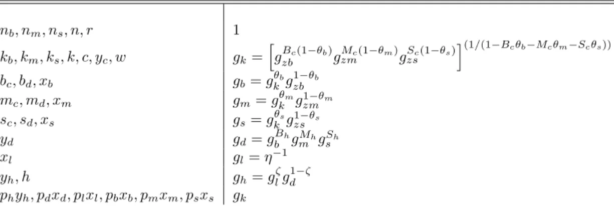
also the case that factor prices display the normal behavior along a balanced growth path: interest rates are stationary while the wage in all sectors is growing at the same rate. The growth rates for the various factors are presented in Table 1 (again see Davis and Heathcote (2005) for details). These growth factors were used to construct a stationary economy; all subsequent discussion is in terms of this transformed economy.
Equilibrium in the economy is described by the vector of factor prices (wt; rt);the vector of
intermediate goods prices,(pbt; pmt; pst);the price of residential investment(pdt), the price of land
Table 1: Growth Rates on the Balanced Growth Path nb; nm; ns; n; r 1 kb; km; ks; k; c; yc; w gk = h gBc(1 b) zb g Mc(1 m) zm gzsSc(1 s) i(1=(1 Bc b Mc m Sc s)) bc; bd; xb gb=gkbg1zb b mc; md; xm gm=gkmg1zmm sc; sd; xs gs=gksgzs1 s yd gd=gbBhgMmhgsSh xl gl= 1 yh; h gh=glg 1 d phyh; pdxd; plxl; pbxb; pmxm; psxs gk
equilibrium prices. In addition, the following quantities are determined in equilibrium: the vector of intermediate goods(xmt; xbt; xst);the vector of labor inputs(nmt; nbt; nst);the total amount of
labor supplied,(nt);the vector of inputs into the …nal goods sectors(bct; bdt; mct; mdt; sct; sdt), the
vector of capital inputs(kmt; kbt; kst);entrepreneurial capital(ket);household investment(kt+1); the vector of …nal goods output (yct; ydt);the technology cuto¤ level (!t); the e¤ective housing
stock(ht+1);and the consumption of households and entrepreneurs(ct; cet):In total, there are 24
quantities to be determined; adding the nine prices, the system is de…ned by 33 unknowns. These are determined by the following conditions:
Factor demand optimality in the intermediate goods markets
rt= i pitxit kit (3equations) (41) wt= (1 i) pitxit nit (3equations) (42)
Factor demand optimality in the …nal goods sector:
pctyct= pbtbct Bc = pmtmct Mc =pstsct Sc (3equations) (43) pdtydt= pbtbdt Bd =pmtmdt Md = pstsdt Sd (3equations) (44)
Factor demand in the housing sector (using the fact that, in equilibriumxlt= 1) produces two more equations: plt pht = y 1 dt st (45) pdt pht = (1 )ydt st (46)
The household’s necessary conditions provide 3 more equations:
1 = Et[(rt+ 1 ) U1(ct+1; ht+1;1 nt+1) U1(ct; ht;1 nt) ]; (47) pht= Et[ U2(ct+1; ht+1;1 nt+1) U1(ct; ht;1 nt) + (1 h)pht+1 U1(ct+1; ht+1;1 nt+1) U1(ct; ht;1 nt) ]; (48) wt= U3(ct; ht;1 nt) U1(ct; ht;1 nt) : (49)
The …nancial contract provides the condition for the markup and the incentive compatibility constraint: st1= " (f(!t; !;t) +g(!t; !;t)) + (!t; !;t) f(!t; !;t) @f(!t; !;t) @!t # (50) phtydt1 =k e t (rt+ 1 ) 1 stg(!t; !;t) st (51)
The entrepreneur’s maximization problem provides the following Euler equation:
1 = Et (rt+1+ 1 )
st+1 f(!t+1; !;t+1) 1 st+1g(!t+1; !;t+1)
(52)
To these optimality conditions, we have the following market clearing conditions: Labor market clearing:
nt= X
i
Market clearing for capital:
kt= X
i
kit; i=b; m; s (54)
Market clearing for intermediate goods:
xbt=bct+bdt; xmt=mct+mdt; xst=sct+sdt: (55)
The aggregate resource constraint for the consumption …nal goods sector (i.e. the law of motion for capital)
kt+1= (1 )kt+yct ct cet (56)
The law of motion for the e¤ective housing units:
ht+1= (1 h)ht+ydt1 (1 (!t) ) (57)
The law of motion for entrepreneur’s capital stock:
kte+1=kte (rt+ 1 )
1 stg(!t; !;t)
stf(!t; !;t) cet (58)
Finally, we have the production functions. Speci…cally, for the intermediate goods markets:
xit=kiti(nitexpzit)1 i; i=b; m; s (59)
For the …nal goods sectors, we have:
Table 2: Key Preference and Production Parameters Depreciation rate for capital: 0.056 Depreciation rate for e¤ective housing(h): h 0.014
Land’s share in new housing: 0.106 Population growth rate: 1.017
Discount factor: 0.951
Risk aversion: 2.00
Consumption’s share in utility: c 0.314
Housing’s share in utility: h 0.044
Leisure’s share in utility: 1- c h 0.642
ydt=bBdtdm Md
dt s Sd
dt (61)
These provide the required 33 equations to solve for equilibrium. In addition there are the laws of motion for the technology shocks and the uncertainty shocks.
~zt+1=B ~zt+~"t+1 (62)
!;t+1= 10 !;texp" ;t+1 (63)
To solve the model, we log linearize around the steady-state. The solution is de…ned by 33 equations in which the endogenous variables are expressed as linear functions of the vector of state variables(zbt; zmt; zst; !t; kt; ket; ht):
4
Calibration and Data
A strong motivation for using the Davis and Heathcote (2005) model is that the theoretical constructs have empirical counterparts. Hence, the model parameters can be calibrated to the data. We use directly the parameter values chosen by the previous authors; readers are directed to their paper for an explanation of their calibration methodology. Parameter values for preferences, depreciation rates, population growth and land’s share are presented in Table 2. In addition, the
Table 3: Intermediate Production Technology Parameters
B M S
Input shares for consumption/investment good(Bc; Mc; Sc) 0.031 0.270 0.700
Input shares for residential investment(Bd; Md; Sd) 0.470 0.238 0.292
Capital’s share in each sector( b; m; s) 0.132 0.309 0.237
Sectoral trend productivity growth(%) (gzb; gzm; gzs) -0.27 2.85 1.65
parameters for the intermediate production technologies are presented in Table 3.17
As in Davis and Heathcote (2005), the exogenous shocks to productivity in the three sectors are assumed to follow an autoregressive process as given in eq. (3). The parameters for the vector autoregression are the same as used in Davis and Heathcote (2005) (see their Table 4, p. 766 for details). In particular, we use the following values (recall that the rows of theBmatrix correspond to the building, manufacturing, and services sectors, respectively):
B= 0 B B B B B B @ 0:707 0:010 0:093 0:006 0:871 0:150 0003 0:028 0:919 1 C C C C C C A
Note this implies that productivity shocks have modest dynamic e¤ects across sectors. The con-temporaneous correlations of the innovations to the shock are given by the correlation matrix:
= 0 B B B B B B @
Corr("b; "b) Corr("b; "m) Corr("b; "s)
Corr("m; "m) Corr("m; "s) Corr("s; "s) 1 C C C C C C A = 0 B B B B B B @ 1 0:089 0:306 1 0:578 1 1 C C C C C C A
The standard deviations for the innovations were assumed to be: ( bb; mm; ss)= (0.041, 0.036,
0.018).
For the …nancial sector, we use the same loan and bankruptcy rates as in Carlstrom and Fuerst (1997) in order to calibrate the steady-state value of!, denoted$;and the steady-state standard
1 7Davis and Heathcote (2005) determine the input shares into the consumption and residential investment good by analyzing the two sub-tables contained in the “Use” table of the 1992 Benchmark NIPA Input-Output tables. Again, the interested reader is directed to their paper for further clari…cation.
deviation of the entrepreneur’s technology shock, 0. The average spread between the prime and commercial paper rates is used to de…ne the average risk premium (rp) associated with loans to entrepreneurs as de…ned in Carlstrom and Fuerst (1997); this average spread is1:87%(expressed as an annual yield). The steady-state bankruptcy rate (br)is given by ($; 0) and Carlstrom and Fuerst (1997) used the value of 3.9% (again, expressed as an annual rate). This yields two equations which determine ($; 0):
($; 0) = 3:90
$ g($; 0)
1 = 1:87 (64)
yielding$ 0:65, 0 0:23.18
Finally, the entrepreneurial discount factor can be recovered by the condition that the steady-state internal rate of return to the entrepreneur is o¤set by their additional discount factor:
sf($; 0) 1 sg($; 0)
= 1
and using the mark-up equation forsin eq. (29), the parameter then satis…es the relation
= gU
gK
1 + ($; 0)
f0($; 0) 0:832
where,gU is the growth rate of marginal utility andgKis the growth rate of consumption (identical
to the growth rate of capital on a balanced growth path). The autoregressive parameter for the risk shocks, , is set to 0.90 so that the persistence is roughly the same as that of the productivity shocks.
Figure 1 and Table 4 show the cyclical and statistical features for the period from 1975 through
1 8Note that the risk premium can be derived from the markup share of the realized output and the amount of pay-ment on borrowing: st!tf pt= (1 +rp) (f pt nwt):And using the optimal factor payment (project investment), f pt;in equation (30), we arrive at the risk premium in equation (64).
Table 4: Business Cycle Properties (1975:1 - 2007:2) Data: all series are Hodrick-Prescott …ltered
with the smoothing parameter set to 1600 % S.D.
GDP 1:2
Consumption 0:69
House Price Index (HPI) 1:9 Non - Residential Fixed Investment (Non-Res) 4:5 Residential Fixed Investment (Res) 8:7 Correlations
GDP, Consumption 0:83
GDP, HPI 0:31
GDP, HPI (for pre 1990) 0:21 GDP, HPI (for post 1990) 0:51
Non-Res, Res 0:29
GDP, Non-Res 0:81
GDP, Res 0:30
GDP, Real Estate Loans (from 1985:1) 0:15 Real Estate Loans, HPI 0:47
Lead - Lag correlations i= 3 i= 0 i= 3
GDPt; N on rest i 0:47 0:78 0:31
GDPt; rest i 0:27 0:20 0:32
N on rest i; rest 0:63 0:26 0:27
the second quarter of 2007 using quarterly data. The U.S. business cycle properties for various aggregate and housing variables are listed in Table (4). As mentioned in the Introduction, the stylized facts for housing are readily seen i): Housing prices are much more volatile than output; ii) Residential investment is almost twice as volatile as non-residential investment; iii) GDP, con-sumption, the price of housing, non-residential - and residential investment all co-move positively; iv) and lastly, residential investment leads output by three quarters.
Table 5: Steady - State Values: Ratios to GDP
Variables Our model Davis and Heathcote Data Data
(D & H) (1948 - 2001) (1948 - 2007)
Capital Stock (K) 1.96 1.52 1.52 1.43
Residential structures stock(Pd S) 3.20 1.00 1.00 1.00
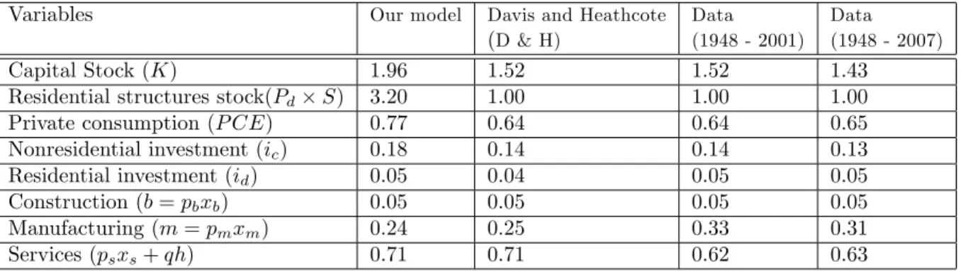
Private consumption (P CE) 0.77 0.64 0.64 0.65 Nonresidential investment(ic) 0.18 0.14 0.14 0.13 Residential investment(id) 0.05 0.04 0.05 0.05 Construction(b=pbxb) 0.05 0.05 0.05 0.05 Manufacturing(m=pmxm) 0.24 0.25 0.33 0.31 Services(psxs+qh) 0.71 0.71 0.62 0.63
5
Results
5.1
Steady State Values, Second Moments and Lead - Lag Patterns
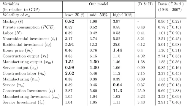
Table 5 shows some of the selected steady-state values from our model that includes the …nancial friction. These steady state values di¤er somewhat from those in Davis and Heathcote (2005) but the calibrated parameter values produce steady-state values that are broadly in line with the data. Our main interest is in the business cycle, i.e. second moment, properties of the model. To examine this, we solve the model for three di¤erent levels of stochastic volatility: a low level in which the innovation to stochastic volatility has a standard deviation of 0.20, a medium level in which the innovation to stochastic volatility has a standard deviation of 0.50;and a high level of volatility in which the innovation to stochastic volatility has a standard deviation of 1.10:19 That is we assume that for the low volatility economy," N(0;0:20);the medium volatility economy has" N(0;0:50)and the high volatility economy has" N(0;1:10):(For all economies the autoregressive parameter for the shock process was held constant at = 0:90.) The results from this exercise are shown in Table 6. We compare the second moments from our economy to that in the Davis and Heathcote (2005) model and to the data. For the last comparison, we present a two-standard deviation range as a crude measure of a 95% con…dence interval.1 9Recent research by Gilchrist et al. (2009) suggests that a relative standard deviation of 110% is not unreason-able.
Table 6: Standard Deviations in ratio to GDP with low volatility of variance
Variables Our model (D & H) Data (+2s.d.)
(in relation to GDP) (1948 - 2007)
Volatility of ! low: 20 % mid: 50% high:110%
Markup (s) 0.82 1.90 3.97 - 0.96 (+0.22) Private consumption (P CE) 0.52 0.52 0.55 0.48 0.78 (+0.15) Labor (N) 0.39 0.42 0.53 0.41 1.01 (+0.20) Nonresidential investment(ic) 3.17 3.74 5.52 3.21 2.51 (+0.45) Residential investment(id) 5.91 12.2 25.0 6.12 5.04 (+0.98) House price(ph) 0.46 0.76 1.44 0.4 1.36 (+0.31) Construction output(xb) 3.85 6.15 11.5 4.02 2.74 (+0.53) Manufacturing output(xm) 1.51 1.50 1.46 1.58 1.85 (+0.36) Service output(xs) 0.98 1.00 1.06 0.99 0.85 (+0.16) Construction labor(nb) 2.62 5.46 11.2 2.15 2.37 (+0.45) Manufacturing(nm) 0.38 0.38 0.39 0.39 1.53 (+0.30) Service(ns) 0.39 0.45 0.64 0.37 0.66 (+0.13) Construction Investment(ib) 2.87 5.60 11.3 25.9 9.69 (+1.88) Manufacturing Investment(im) 1.05 1.04 1.02 3.23 3.53 (+0.69) Service Investment(is) 1.04 1.05 1.11 3.43 2.91 (+0.46)
Note that when the stochastic volatility in the housing sector is low, the model basically replicates the frictionless economy which, in turn, is consistent with many features seen in the data. However, a glaring inconsistency from the low volatility economy is the behavior of housing prices: the model severely underpredicts the volatility of housing prices. The model improves in this dimension as stochastic volatility in the housing sector increases and, in the high volatility economy, the model comes close to the matching the observed volatility. But success in this dimension comes at a cost in that the volatility of residential investment is over …ve times greater than that seen in the data. The Davis and Heathcote model makes the strong assumption of no investment adjustment costs and relaxing this assumption would moderate the volatility in residential investment.
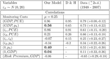
The contemporaneous correlations of several key variables are presented in Table 7 (for expo-sitional purposes, we only report that values for the low volatility economy (" N(0;0:20))as the correlations were consistent across the three model economies). All variables co-move posi-tively with the exception of house price and residential investment. This inconsistency with the
Table 7: Correlations
Variables Our Model D & H Data (+2s.d.)
" N(0;20) (1948 - 2007) Correlations Monitoring Costs = 0:25 (GDP; P CE) 0.96 0.95 0.79 (+0.08,-0.12) (GDP; ph) 0.56 0.65 0.73 (+0.13,-0.22) (ic; P CE) 0.86 0.91 0.61 (+0.15,–0.20) (id; P CE) 0.21 0.26 0.66 (+0.13,-0.18) (ic; id) -0.07 0.15 0.25 (+0.23,-0.27) (id; ph) -0.34 -0.2 0.34 (+0.22,-0.26) (s; ph) 0.40 - 0.55 (+0.21,-0.30) (s; GDP) 0.04 - 0.11 (+0.33,-0.36) (Risk P remium; GDP) -0.06 - -0.65 (+0.29,-0.18)
data is not surprising in that the shocks to our model economy all emanate from the supply side whereas demand shocks (say in the form of easier access to credit for home buyers) no doubt play an important role in the behavior of the actual data. Our model critically has predictions for two variables that are not present in the Davis and Heathcote (2005) model: namely, the housing markup parameter, st, and the risk premium associated with loans to housing producers. The
time series for these two variables are presented in Figure 4. It is clear that the housing markup is procyclical while the risk premium is countercyclical. As reported in Table 7, the model with …nancial frictions can replicate these features, although the risk premium is only mildly counter-cyclical. The model’s ability to replicate these two features provides a compelling argument for the inclusion of a credit market.
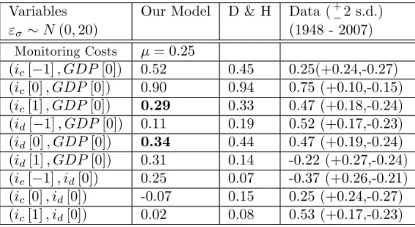
The last set of housing stylized facts that is in question is the lead - lag patterns of residential and non-residential investments. Table 8 shows the results. As in Davis and Heathcote (2005), we also fail to reproduce this feature of the data. Consequently, the propagation mechanism of agency costs model does amplify prices and other real variables, but does not contribute in explaining the lead-lag features.
Table 8: Lead - Lag Patterns: Annual Frequency Variables Our Model D & H Data (+2 s.d.)
" N(0;20) (1948 - 2007) Monitoring Costs = 0:25 (ic[ 1]; GDP[0]) 0.52 0.45 0.25(+0.24,-0.27) (ic[0]; GDP[0]) 0.90 0.94 0.75 (+0.10,-0.15) (ic[1]; GDP[0]) 0.29 0.33 0.47 (+0.18,-0.24) (id[ 1]; GDP[0]) 0.11 0.19 0.52 (+0.17,-0.23) (id[0]; GDP[0]) 0.34 0.44 0.47 (+0.19,-0.24) (id[1]; GDP[0]) 0.31 0.14 -0.22 (+0.27,-0.24) (ic[ 1]; id[0]) 0.25 0.07 -0.37 (+0.26,-0.21) (ic[0]; id[0]) -0.07 0.15 0.25 (+0.24,-0.27) (ic[1]; id[0]) 0.02 0.08 0.53 (+0.17,-0.23)
5.2
Dynamics: Impulse Response Functions
While the results discussed above provide some support for the housing cum credit channel model, the role of the lending channel is not easily seen because of the presence of the other impulse shocks (i.e., the sectoral productivity shocks). To analyze how the lending channel in‡uences the e¤ects of a risk shock, we analyze the model’s impulse response functions to risk shocks under two di¤erent scenarios. In the …rst scenario, we set the monitoring cost parameter to zero ( = 0) while in the second scenario we use the value employed in the stochastic simulations( = 0:25):
With no monitoring costs, risk shocks should not in‡uence the behavior of housing prices and residential investment (see eqs. (29);(45); and(46):We also examine the economy’s response to an innovation to productivity in the construction sector (this being the most important input into the residential investment good). The impulse response functions (to a 1% innovation in both shocks) for a selected set of key variables are presented in Figures 7-9.
We …rst turn to the behavior of three key macroeconomic variables, namely GDP, household consumption (denoted PCE), and residential investment (denoted RESI) seen in Figure 7. The response to a technology shock to the construction sector has the predicted e¤ect that GDP increases. On the other hand, consumption falls slightly while residential investment increases; this re‡ects agents response to the expected high productivity (due to the persistence of the shock)
in the construction sector. Note that the response in residential investment is much larger than in the other two variables since this sector is most a¤ected by the greater productivity in this critical input. Also note that monitoring costs (i.e. whether = 0or = 0:25) play a rather insigni…cant role in the dynamic e¤ects of a technology shock. And, as the model implies, when = 0, risk shocks have no e¤ect on the economy. (For this reason, in Figures 8 and 9, we report only the responses for = 0:25.) When = 0:25;a risk shock which a¤ects housing production results in a modest fall in GDP but a relatively dramatic fall in residential investment. Recall, as discussed in the partial equilibrium analysis of the credit channel model, an increase in productivity risk results in a leftward shift in the supply of housing; since residential investment is the primary input into housing, it too falls in response to the increased risk. Consumption responds positively which is consistent with models that have an investment speci…c technology shock (e.g. Greenwood, Hercowitz, and Krusell (2000)).
Figure 8 reports the impulse response functions of the housing markup, the risk premium on loans to the housing producers and the bankruptcy rate. A positive technology shock to the construction sector increases the demand for housing and, ceteris paribus, will result in an increase in the price of housing. This will result in greater lending to the housing producers which will result in a greater bankruptcy rate and risk premium; both of these e¤ects imply that the housing markup will increase. Note the counterfactual implication that both the bankruptcy rate and the risk premium on loans will be procyclical; this was also the case in the original Carlstrom and Fuerst (1997) model and for exactly the same reason. In contrast, a risk shock produces countercyclical behavior in these three variables. Hence, this argues for inclusion of risk shocks as an important impulse mechanism in the economy.
Finally, we report in Figure 9, the impulse response functions of the prices of land and housing to the two shocks. A technology shock to the construction sector results in lower cost of housing inputs due to the increased output in residential investment so that the price of housing falls. However, the price of land, i.e. the …xed factor, increases. For an uncertainty shock, the resulting
fall in the supply of housing causes the demand for the …xed factor (land) to fall and the price of the …nal good (housing) to increase.
In ending this section, a word of caution is needed in interpreting the quantitative magnitudes seen in the impulse response functions. In particular, note that the response of housing prices to a productivity increase in the construction sector is greater than the response due to a risk shock. One might deduce that the housing sector and risks shocks play a minor role in the movement of housing prices. As the results from the full model (i.e. when the all technology and risk shocks are present) imply, such a conclusion would be incorrect (see Table 6).
5.3
Some Final Remarks
Our primary …ndings fall into two broad categories. First, risk shocks to the housing produc-ing sector imply a quantitatively large role for uncertainty over the housproduc-ing and business cycles. Second, our model can account for most of the salient features of housing stylized facts, in par-ticular, housing prices are more volatile than output. The lead - lag pattern of residential and non-residential, however, is still not reconciled within our framework.20
For future research, modelling uncertainty due to time variation in the types of entrepreneurs would be fruitful. One possibility would be an economy with a low risk agent whose productivity shocks exhibit low variance and a high risk agent with a high variance of productivity shocks. Because of restrictions on the types of …nancial contracts that can be o¤ered, the equilibrium is a pooling equilibrium so that the same type of …nancial contract is o¤ered to both types of agents. Hence the aggregate distribution for technology shocks hitting the entrepreneurial sector is a mixture of the underlying distributions for each type of agent. Our conjecture is that this form of uncertainty has important quantitative predictions and, hence, could be an important impulse mechanism in the credit channel literature that, heretofore, has been overlooked. It also anecdotally corresponds with explanations for the cause of the current credit crisis: a substantial
2 0 Recently, Jonas Fisher (2007) presents a model with household production which does produce the lead-lag pattern pattern observed in residential and non-residential investment.
References
Aoki, Kosuke, J. Proudman, and J. Vlieghe, (2004), “House Prices, Consumption, and Monetary Policy: A Financial Accelerator Approach.”Journal of Financial Intermediation, 13(4), pp. 414–35.
Bloom, N., M. Floetotto and N. Jaimovich, (2008), “Really Uncertain Business Cycles,” Stanford University Working Paper.
Carlstrom, C.T. and T.S. Fuerst, (1997), “Agency Costs, Net Worth, and Business Fluctu-ations: A Computable General Equilibrium Analysis,”American Economic Review, 87, pp. 893 - 910.
Carlstrom, C.T. and T.S. Fuerst, (1998),“Agency Costs and Business Cycles,”, Economic Theory (12), pp. 583-597.
Chari V., Kehoe P. and Ellen R. McGrattan, (2007), "Business Cycles Accounting", forth-coming inEconometrica.
Christiano, L., R. Motto, and M. Rostagno, (2003), “The Great Depression and the Friedman-Schwartz Hypothesis,”Journal of Money, Credit, and Banking, 35, 1119-1198 Christiano, L., R. Motto, and M. Rostagno, (2008), “Financial Factors in Business Cycles", working paper.
Davis, Morris and J. Heathcote, (2005), "Housing and the Business Cycle", International Economic Review, Vol. 46, No. 3, pp. 751 - 784.
Dorofeenko, V., G. Lee and K. Salyer, (2008), “Time Varying Uncertainty and the Credit Channel”,Bulletin of Economic Research, 60:4, pp. 375-403
Fernández-Villaverde, J., P. A. Guerrón-Quintana, J. Rubio-Ramirez, and M Uribe, (2009), “Risk Matters: The Real E¤ects of Volatility Shocks,” NBER Working Paper 14875. Jonas D. M. Fisher, (2007), “Why Does Household Investment Lead Business Investment over the Business Cycle?,”Journal of Political Economy, 115, pp. 141-168.
Kahn, J.A., (2008), “What Drives Housing Prices,”New York Federal Reserve Sta¤ Report no. 345.
Gilchrist, S., J. Sim, and E. Zakrajsek, (2008), “Uncertainty, Credit Spreads, and Investment Dynamics,” FRB Working Paper.
Glaser, E. L. and J. Gyourko, (2006),“Housing Dynamics”, NBER Working Paper No.12787. Greenwood, J., Hercowitz, Z. and Krusell, P. (2000). “The Role of Investment Speci…c Technological Change in the Business Cycle”,European Economic Review, 44, pp. 91–115. Iacoviello, Matteo, "House Prices, Borrowing Constraints and Monetary Policy in the Busi-ness Cycle" (2005),American Economic Review, Vol. 95, No. 3 (June), pp. 739-764. Iacoviello,Matteo and Raoul Minetti,(2008), "The Credit Channel of Monetary Policy: Ev-idence from the Housing Market" (forthcoming),Journal of Macroeconomics.
Iacoviello, Matteo and S.Neri, (2008), "Housing Market Spillovers: Evidence from an Esti-mated DSGE model", Boston College,Department of Economics, mimeo.
6
Data Appendix
Loans: Federal Reserve Board, Statistics: Releases and Historical Data Assets and Liabilities of Commercial Banks in the U.S. - h.8. Seasonally adjusted, adjusted for mergers, billions of dollars. http://www.federalreserve.gov/releases/h8/data.htm
–Total Loans: Total loans and leases at commercial banks.
–Residential Real Estate Loans: Loans to residential sector excluding revolving home equity loans.
–Commercial Real Estate Loans: Loans to commercial sector excluding revolving home equity loans.
–Commercial and Industrial Loans (Business Loans): Commercial and industrial loans at all Commercial Banks.
–Consumer Loans: Consumer (Individual) loans at all commercial banks.
Gross Domestic Product (GDP), Personal Consumption Expenditures (PCE), Aggregate of gross private domestic investment (Non-RESI), Residential gross private domestic investment (RESI), and the Price Indexes for private residential Investment (PRESI) are all from the National Income and Product Accounts Tables (NIPA) at the Bureau of Economic Analysis.
–To calculate the implied markup, s, we used the house price index (HPI), residential investment (RESI) and the price for the RESI (PRESI).
–We use the equationpht= (1 )ydt pdtst:
House Price Index. (HPI): Constructed based on conventional conforming mortgage trans-actions obtained from the Federal Home Loan Mortgage Corporation(Freddie Mac) and the Federal National Mortgage Association (Fannie Mae). Source: The O¢ ce of Federal Housing Enterprise Oversight (OFHEO).
Risk Premium: To calculate our risk premium, we used the spread between the prime rate and the three month commercial paper. These data can be obtained from Federal Reserve Bank of St. Louis, FRED Dataset under the category of Interest Rates.
–http://research.stlouisfed.org/fred2/categories/22. These two series are monthly.
–Commercial rate: CP3M, 3-Month Commercial Paper Rate :1971-04 till 1997-08.
Figure 1: U.S. GDP, House Price, Non – and Residential Fixed Investments (1975:1 –
2007:2)
-6 -4 -2 0 2 4 6 8 1975 1980 1985 1990 1995 2000 2005 GDP (s.d. = 1.2)House Price Index (HPI) (s.d.= 1.9) Percent Deviation from Trend (using HP filter) for U.S. Output and House Prices Quarterly (1975:1 - 2007:2)
2006:1
corr (GDP, HPI) = 0.31
corr (GDP, HPI) = 0.21 for pre 1990 corr (GDP, HPI) = 0.51 for post 1990
-30 -20 -10 0 10 20 1975 1980 1985 1990 1995 2000 2005
Non-residential fixed investment (s.d. = 4.5) Residential Fixed Investment (s.d.= 8.7) Percent Deviation from Trend (using HP filter)
for U.S. Fixed Private Non- and Residential Investment Quarterly (1975:1 - 2007:2)
2005:3
corr (Non Res, Res Inv) = 0.29
-30 -20 -10 0 10 20 1975 1980 1985 1990 1995 2000 2005 GDP (s.d. = 1.2)
Non-residential fixed investment (s.d. = 4.5) Residential Fixed Investment (s.d.= 8.7) Percent Deviation from Trend (using HP filter)
for U.S. GDP, Fixed Private Non- and Residential Investment Quarterly (1975:1 - 2007:2)
corr (GDP, Non-Res Inv.) = 0.81 corr (GDP, Res Inv) = 0.3 corr (Non Res, Res Inv) = 0.29
Figure 2: Different Loans at All U.S. Commercial Banks (1990:1 to 2007:7)
0
500
1000
1500
2000
2500
3000
3500
4000
90
92
94
96
98
00
02
04
06
Commercial and Industrial
Individual (Consumer)
Residential Real Estate
Commercial Real Estate
in
Billio
n
s
o
f Do
lla
rs
Figure 3: U.S. GDP, House Price and Residential Real Estate Loans
-6
-4
-2
0
2
4
6
-.04
-.02
.00
.02
.04
.06
1975
1980
1985
1990
1995
2000
2005
GDP
REAL ESTATE LOANS (Right Scale)
HOUSE PRICE INDEX
Corr( GDP,LOAN)= 0.15
Corr(HOUSE PRICE,LOAN)= 0.47
Percent Deviation from trend (using HP filter):
U.S. Output Real Estate Loans and Price
5.6
6.0
6.4
6.8
7.2
7.6
8.0
0
100
200
300
400
500
600
1975
1980
1985
1990
1995
2000
2005
Residential Real Estate Loans (in logs)
House Price Index (Right Scale)
Figure 4: House Price, Housing Markups, and Risk Premium
-.12
-.08
-.04
.00
.04
.08
1970 1975 1980 1985 1990 1995 2000 2005
Markup
House Price
correlation: 0.52
House Price vs Markup: Annual 1970 - 2008 (HP filtered)
-.06
-.04
-.02
.00
.02
.04
.06
-1.2
-0.8
-0.4
0.0
0.4
0.8
1.2
1970 1975 1980 1985 1990 1995 2000 2005
GDP
Risk Premium
correlation: -0.65 over the common sample
GDP vs Risk Premium: Annual 1970 - 2008 (HP filtered)
GD
P
Ris
k
Pr
e
m
iu
m
Figure 5: Flow of Funds in Credit Channel with Housing Model
(Government, Households l
and incom
e, as well as Entr
epreneur labor input an
d in
co
m
e are not shown)
38
Real Estat
e
Developers/Entrepreneurs
(produce houses)
Savings
Capital
Labor
Capital
Pay off
Loans
Loans
Capital
(Solvent)
Invest
Loans +
Net
Wor
th
Incom
e
Capital
(Bankrupt)
Banking
Households
Monitoring
Interm
ediate
Firm
s
Costs
Residential
Investm
ent
+
Land
Houses: Housing
Sector
Construction
Manufacturin
g
Service
Consum
ption/
Capital
Final Goods Firm
Figure 6: Technology and Uncertainty Shocks:
Effects on Housing Demand and Supply
A
B
Markup
Price
House
C
Technology shock: A to B Uncertainty shock: A to C HousesFigure 7: Response of Output, Private Consumption Expenditure, and Investment
to 1% increase in Sector (Construction) Technology shocks and Uncertainty
Shocks
(percentage deviations from steady-state values)
Technology Shock to Construction sector
Uncertainty Shock to Housing Developer
m
= 0.25 (monitoring cost: effects of agency cost)
m
= 0 (no monitoring cost: multi-sector model with housing and no agency cost)
Figure 8: Response of Markup House Price, Risk Premia, and Bankruptcy Rate to a
1% increase in Sector (Construction) Technology shocks and Uncertainty Shocks
(percentage deviations from steady-state values)
Technology Shock to Construction sector
Uncertainty Shock to Housing Developer
m
= 0.25 (monitoring cost: effects of agency cost)
m
= 0 (no monitoring cost: multi-sector model with housing and no agency cost)
Figure 9: Response of Land and House Prices, and Interest Rate to a 1% increase in
increase in Sector (Construction) Technology Shocks and Uncertainty Shocks
(percentage deviations from steady-state values)
Technology Shock to Construction sector
Uncertainty Shock to Housing Developer
m
= 0.25 (monitoring cost: effects of agency cost)
Authors:Victor Dorofeenko, Gabriel S. Lee, Kevin D. Salyer Title: Risk Shocks and Housing Markets
Reihe Ökonomie / Economics Series 249 Editor: Robert M. Kunst (Econometrics)
Associate Editors: Walter Fisher (Macroeconomics), Klaus Ritzberger (Microeconomics) ISSN: 1605-7996
© 2010 by the Department of Economics and Finance, Institute for Advanced Studies (IHS),